Equivalence of Domains for Hyperbolic Hubbard-Stratonovich Transformations

Abstract

We settle a long standing issue concerning the traditional derivation of non-compact non-linear sigma models in the theory of disordered electron systems: the hyperbolic Hubbard-Stratonovich (HS) transformation of Pruisken-Schäfer type. Only recently the validity of such transformations was proved in the case of $U(p,q)$ (non-compact unitary) and $O(p,q)$ (non-compact orthogonal) symmetry. In this article we give a proof for general non-compact symmetry groups. Moreover, we show that the Pruisken-Schäfer type transformations are related to other variants of the HS transformation by deformation of the domain of integration. In particular we clarify the origin of surprising sign factors which were recently discovered in the case of orthogonal symmetry.

1 Introduction

Non-compact non-linear sigma models are an important and extensively used tool in the study of disordered electron systems. The relevant formalism was pioneered by Wegner [1], Schäfer & Wegner [2], and Pruisken & Schäfer [3]. Efetov [4] improved the formalism by developing the supersymmetry method to derive non-linear sigma models. Many applications of the supersymmetry method can be found in the textbook by Efetov [5].

There exist different ways to derive non-linear sigma models from microscopic models; for an introduction see [6]. One step in the traditional approach uses a Hubbard-Stratonovich transformation, i.e., a transformation of the form

$$c_{0}\,e^{-\operatorname{Tr}A^{2}}=\int_{\mathrm{D}}e^{-\operatorname{Tr}Q^{2}-2i\operatorname{Tr}QA}|dQ|,$$ (1)

where $c_{0}\in\mathbb{C}$ and the domain of integration D is left unspecified for now. $|dQ|$ denotes Lebesgue measure of a normed vector space.

For the case of compact symmetries the transformation is just a trivial Gaussian integral. To give an indication of the difficulty which arises in the case of a non-compact symmetry (also known as the boson-boson sector of Efetov’s supersymmetry formalism) let us briefly discuss the example of orthogonal symmetry $O(p,q)$. There, $A$ is given by $A_{ij}=\sum_{a=1}^{N}\Phi_{a,i}\Phi_{a,j}s_{jj}$ with $s=\mathrm{Diag}(\mathbbm{1}_{p},-\mathbbm{1}_{q})$ and $\Phi_{a,j}\in\mathbb{R}$. The $\Phi_{a,j}$ represent the microscopic degrees of freedom. Using equation (1) and integrating out $\Phi$ gives a description in terms of the effective degrees of freedom $Q$. The task is to find a domain of integration D for which identity (1) holds and the term $\exp(-2i\operatorname{Tr}QA)$ stays bounded. The latter condition is imposed in order for Fubini’s theorem to apply, as further execution of the Wegner-Efetov formalism calls for the $\Phi$ and $Q$ integrals to be interchanged. Note that the real matrices $A$ obey the symmetry relation $A=sA^{t}s$. A naive choice of integration domain D keeping the term $\exp(-2i\operatorname{Tr}QA)$ bounded would be the domain of all real matrices satisfying $Q=sQ^{t}s$. Unfortunately, this choice of D is not a valid choice in the context of the integral (1) as it renders the quadratic form $\operatorname{Tr}Q^{2}=\operatorname{Tr}QsQ^{t}s$ of indefinite sign.

Schäfer and Wegner (SW) [2] suggested a domain and showed that it solves the difficulty. Yet, a different domain was proposed in later work by Pruisken and Schäfer (PS) [3]. Until recently the mathematical status of identity (1) for the PS domain was unclear. The main obstacle in proving (1) for the PS domain is the existence of a boundary. This precludes an easy proof by completing the square and shifting the contour (as is possible for the standard Gauss integral and for the SW domain). Nevertheless, the PS domain was used in most applications worked out by the mesoscopic and disordered physics community; an early and influential paper of this kind is [10]. Most likely, the reason is that it is easier to do calculations with, as it is invariant under the full symmetry group of the domain of matrices $A$.

Recently Fyodorov, Wei and Zirnbauer in a series of papers [7, 8, 9] proved the PS variant of the HS transformation for the special cases of unitary and orthogonal symmetry. In this article we extend the results to more general symmetry groups. Moreover, our proof clarifies the relation between the PS transformation, the SW transformation and the standard Gaussian integrals. It is shown that the different integrals can be transformed into each other by deforming the domain of integration without changing the value of the integral.

Here is a guide to reading: In section 2 we define the setting and state our main result in the form of a theorem. In addition, we give two corollaries which relate more directly to previous results. In section 3 we apply our results to three different symmetry classes. In particular, previous results concerning the cases of unitary and orthogonal symmetry are reproduced. The proof of the theorem is contained in section 4, which is divided into three subsections. For the convenience of the reader each subsection is preceded by a short introduction of notation, essential structures, and a lemma containing the results of the pertinent part of the proof. The last subsection of section 4 deals with the two corollaries.

2 Statement of result

All constructions take place in $\mathfrak{gl}(n,\mathbb{C})$, the Lie algebra of complex $n\times n$ matrices. [Please be advised however that the following results also apply to the case where $\mathfrak{gl}(n,\mathbb{C})$ is replaced by a complex reductive Lie subalgebra of $\mathfrak{gl}(n,\mathbb{C})$.] Let $s\in\mathfrak{gl}(n,\mathbb{C})$ be hermitian with the property $s^{2}=\mathbbm{1}$. This matrix $s$ gives rise to two involutions $\theta(X)=sXs^{-1}$ and $\gamma(X)=-sX^{\dagger}s^{-1}$ on $\mathfrak{gl}(n,\mathbb{C})$. ‘Involution’ here means an involutive Lie algebra automorphism. For greater generality we allow for further involutions $\tau_{i}$ to be present on $\mathfrak{gl}(n,\mathbb{C})$. Two requirements have to be fulfilled: Firstly, all involutions have to commute with each other and secondly, $s$ has to be in the plus or minus eigenspace of each $\tau_{i}$, i.e. $s=\eta_{i}\tau_{i}(s)$ with $\eta_{i}\in\{\pm 1\}$.

The fixed point set of $\gamma$ and the $\tau_{i}$’s is the real Lie algebra

$$\mathfrak{g}=\{X\in\mathfrak{gl}(n,\mathbb{C})\mid X=\gamma(X)\;\mathrm{and}\;\forall i\;:\;X=\tau_{i}(X)\}.$$

We also introduce the real vector space

$$\mathcal{Q}=\{Q\in\mathfrak{gl}(n,\mathbb{C})\mid Q=-\gamma(Q)\;\mathrm{and}\;\forall i\;:\;\,Q=\eta_{i}\tau_{i}(Q)\},$$

which is an $\mathbb{R}$-module for the adjoint (or commutator) action by $\mathfrak{g}$.

Due to $(\theta\circ\gamma)(X)=-X^{\dagger}$, the decompositions of $\mathfrak{g}$ and $\mathcal{Q}$ into the plus and minus one eigenspaces of $\theta$ are decompositions into hermitian and antihermitian parts. We write these decompositions as $\mathfrak{g}=\mathfrak{k}\oplus\mathfrak{p}$ and $\mathcal{Q}=\mathcal{Q}_{+}\oplus\mathcal{Q}_{-}$, where $\mathfrak{k}$ and $\mathcal{Q}_{+}$ are in the plus one eigenspace and $\mathfrak{p}$ and $\mathcal{Q}_{-}$ are in the minus one eigenspace. $\mathfrak{k}$ and $\mathcal{Q}_{-}$ consist of antihermitian matrices whereas $\mathfrak{p}$ and $\mathcal{Q}_{+}$ consist of hermitian matrices. The commutation relations among all these spaces,

$$\begin{matrix}[l][\mathfrak{k},\mathfrak{k}]\subset\mathfrak{k},&[\mathfrak{k},\mathfrak{p}]\subset\mathfrak{p},&[\mathfrak{p},\mathfrak{p}]\subset\mathfrak{k},&[\mathcal{Q}_{+}\,,\mathcal{Q}_{-}]\subset\mathfrak{p},\\ [\mathcal{Q}_{\pm}\,,\mathcal{Q}_{\pm}]\subset\mathfrak{k},&[\mathfrak{k},\mathcal{Q}_{\pm}]\subset\mathcal{Q}_{\pm}\,,&[\mathfrak{p},\mathcal{Q}_{\pm}]\subset\mathcal{Q}_{\mp}\,,\end{matrix}$$

imply that $\mathfrak{g}\oplus\mathcal{Q}$ is a Lie algebra. (This Lie subalgebra of $\mathfrak{gl}(n,\mathbb{C})$ could have served as the starting point of our setting.) By the definition of $\mathcal{Q}$ the matrix $As$ is hermitian for all $A\in\mathcal{Q}$. Note that $s\in\mathcal{Q}_{+}$. To preclude any pathologies that might otherwise occur, we demand that the Lie group $\exp(\mathfrak{k})$ be closed.

The parametrization of the Pruisken-Schäfer domain is given by

$$PS:\;\mathfrak{p}\oplus\mathcal{Q}_{+} \rightarrow\mathcal{Q},$$

$$(Y,X) \mapsto e^{Y}Xe^{-Y}.$$ (2)

The standard domain for a Gaussian integral is called ‘Euclidean’ in the following. It is parametrized by

$$Euclid:\; \mathcal{Q}_{-}\oplus\mathcal{Q}_{+}\rightarrow\mathcal{Q}^{\mathbb{C}},$$

$$(\tilde{Y},X)\mapsto X+i\tilde{Y},$$

where $\mathcal{Q}^{\mathbb{C}}=\mathcal{Q}\oplus i\mathcal{Q}$. Finally, the parametrization of the one-parameter family of Schäfer-Wegner domains is given by

$$SW:\;\mathfrak{p}\oplus\mathcal{Q}_{+} \rightarrow\mathcal{Q}^{\mathbb{C}},$$

$$(Y,X) \mapsto X-ibe^{Y}se^{-Y},$$ (3)

where $b$ is any positive real number.

The following statement relies on making a choice of orientation for the PS domain. (Note that no such choice is made for D in (1).) Once and for all we now fix an orientation for each of the vector spaces $\mathcal{Q}_{+}$, $\mathfrak{p}$, and $\mathcal{Q}_{-}$. By viewing $PS$, $Euclid$, and $SW$ as orientation-preserving maps, we then have orientations on the corresponding domains of integration.

Theorem 2.1.

Let $A\in\mathcal{Q}$ in the setting above. If $As>0$ one has

$$\lim_{\epsilon\rightarrow 0}\int_{PS}e^{-\operatorname{Tr}(Q^{2})-2i\operatorname{Tr}(QA)}\chi_{\epsilon}(Q)dQ=c\,e^{-\operatorname{Tr}(A^{2})}.$$

Here, $\chi_{\epsilon}(Q)=\exp(\frac{\epsilon}{4}\operatorname{Tr}[Q-\theta(Q)]^{2})\leq 1$ is a regulating function ($\epsilon>0$) and $dQ$ denotes a constant volume form (i.e. a constant differential form of top degree) on $\mathcal{Q}$. The normalization constant $c\in\mathbb{C}\setminus\{0\}$ does not depend on $A$.

The main idea of the proof is to show that the PS domain can be extended by a nulldomain (of holomorphic continuation of $dQ$) and then deformed into a Euclidean domain without changing the value of the integral. Appendix B shows that one can also deform the SW domain into this Euclidean domain. Thus the PS and SW domains are deformations of the same Euclidean domain.

Now we formulate two corollaries. For that purpose let $\mathfrak{h}$ be a maximal Abelian subalgebra $\mathfrak{h}\subset\mathcal{Q}_{+}\subset\mathfrak{gl}(n,\mathbb{C})$. We require that $s\in\mathfrak{h}$. Let $\Sigma_{+}(\mathfrak{k}\oplus\mathcal{Q}_{+},\mathfrak{h})$ denote a set of positive roots of the adjoint action of $\mathfrak{h}$ on $\mathfrak{k}\oplus\mathcal{Q}_{+}$. Similarly $\Sigma_{+}(\mathfrak{p}\oplus\mathcal{Q}_{-},\mathfrak{h})$ denotes a set of positive roots of the adjoint action of $\mathfrak{h}$ on $\mathfrak{p}\oplus\mathcal{Q}_{-}$. The multiplicity of a root $\alpha$ is denoted by $d_{\alpha}$.

The following corollary is the analogue of corollary 1 in [9].

Corollary 2.1.

Let $|dg|$ denote Haar measure of the closed analytic subgroup $G\subset GL(n,\mathbb{C})$ with Lie algebra $\mathfrak{g}$. We then have

$$\lim_{\epsilon\rightarrow 0}\int_{\mathfrak{h}}\left(\int_{G}e^{-2i\operatorname{Tr}(g\lambda g^{-1}A)}\chi_{\epsilon}(g\lambda g^{-1})|dg|\right)e^{-\operatorname{Tr}\lambda^{2}}J^{\prime}(\lambda)|d\lambda|=\tilde{c}\,e^{-\operatorname{Tr}(A^{2})},$$

where $|d\lambda|$ denotes Lebesgue measure on the vector space $\mathfrak{h}$ and

$$J^{\prime}(\lambda)=\prod_{\alpha\in\Sigma_{+}(\mathfrak{k}\oplus\mathcal{Q}_{+},\mathfrak{h})}|\alpha(\lambda)|^{d_{\alpha}}\prod_{\alpha\in\Sigma_{+}(\mathfrak{p}\oplus\mathcal{Q}_{-},\mathfrak{h})}\alpha(\lambda)^{d_{\alpha}}.$$

The constant $\tilde{c}\in\mathbb{C}\setminus\{0\}$ does not depend on $A$.

Remark 2.1.

It is particularly noteworthy that for odd multiplicities $d_{\alpha}$ of roots $\alpha\in\Sigma_{+}(\mathfrak{p}\oplus\mathcal{Q}_{-},\mathfrak{h})$ the ‘Jacobian’ $J^{\prime}(\lambda)$ is not positive but has alternating sign.

The following corollary is the analogue of theorem 1 in [9]:

Corollary 2.2.

If the parametrization $PS$ is nearly everywhere injective and regular, then

$$\lim_{\epsilon\rightarrow 0}\int_{\mathrm{Im}PS}e^{-\operatorname{Tr}(Q^{2})-2i\operatorname{Tr}(QA)}\chi_{\epsilon}(Q)\operatorname{sgn}(J^{\prime}(\lambda))|dQ|=\tilde{c}^{\prime}e^{-\operatorname{Tr}(A^{2})}.$$

Here $\mathrm{Im}PS=PS$ denotes the non-oriented image of $PS$. The mapping from $\mathrm{Im}PS$ to $\mathfrak{h}$ sending $Q$ to $\lambda$ is well defined up to a set of measure zero. $|dQ|$ denotes Lebesgue measure on $\mathcal{Q}$, and $\tilde{c}^{\prime}\in\mathbb{C}\setminus\{0\}$ is a constant which does not depend on $A$.

Remark 2.2.

While we believe that the assumptions on $PS$ in corollary 2.2 follow from the general setting, we have not been able to find a proof thereof.

3 Examples

First we reproduce the examples of unitary and orthogonal symmetry. For this we calculate $J^{\prime}$ and apply corollary 2.1.

3.1 $U(p,q)$ symmetry

This case has been handled by Fyodorov [7] using different methods. To apply the general theorem (2.1) we work in the complex Lie algebra $\mathfrak{gl}(p+q,\mathbb{C})$ and define $s=\mathrm{Diag}(\mathbbm{1}_{p},-\mathbbm{1}_{q})$. No additional involutions $\tau_{i}$ are needed. We have

$$\mathfrak{k}\oplus\mathcal{Q}_{+}=\{x\in\mathfrak{gl}(n,\mathbb{C})\mid X=sXs\},\quad\mathfrak{p}\oplus\mathcal{Q}_{-}=\{x\in\mathfrak{gl}(n,\mathbb{C})\mid X=-sXs\}.$$

The maximal Abelian subalgebra $\mathfrak{h}\subset\mathcal{Q}_{+}$ is spanned by the real diagonal matrices. Let $\lambda:=\mathrm{Diag}(\lambda_{1},\dots,\lambda_{p+q})\in\mathfrak{h}$ be such a matrix. The roots $\Sigma_{+}(\mathfrak{gl}(p+q),\mathfrak{h})$ are given by $f_{i}-f_{j}$ where $i<j$ and $f_{i}(\lambda)=\lambda_{i}$. For $i\leq p<j\leq p+q$ the roots $f_{i}-f_{j}$ are elements of $\Sigma_{+}(\mathfrak{p}\oplus\mathcal{Q}_{-},\mathfrak{h})$, otherwise they are elements of $\Sigma_{+}(\mathfrak{k}\oplus\mathcal{Q}_{+},\mathfrak{h})$.

The root space corresponding to $f_{i}-f_{j}$ is $\mathbb{C}E_{ij}$ where $E_{ij}$ is the matrix with unity in the $ij$ position and zero elsewhere. Thus every root space has complex dimension one, or real dimension two. Hence

$$J^{\prime}(\lambda)=\prod_{i<j}|\lambda_{i}-\lambda_{j}|^{2}.$$

With this expression for $J^{\prime}(\lambda)$ the formula of corollary 2.1 agrees with that of Fyodorov [7].

3.2 $O(p,q)$ symmetry

This case has been dealt with by Fyodorov, Wei and Zirnbauer [9]. In addition to the involutions of the unitary setting we need an involution $\tau_{1}(X)=-sX^{t}s$ and $\eta_{1}=-1$. The additional presence of this involution requires all matrices to be real. In consequence, all root spaces are now one dimensional, and they give rise to non-trivial signs:

$$J^{\prime}(\lambda) =\prod_{\alpha\in\Sigma_{+}(\mathfrak{p}\oplus\mathcal{Q}_{-},\mathfrak{h})}\alpha(\lambda)\prod_{\alpha\in\Sigma_{+}(\mathfrak{k}\oplus\mathcal{Q}_{+},\mathfrak{h})}|\alpha(\lambda)|$$

$$=\prod_{i\leq p<j\leq p+q}(\lambda_{i}-\lambda_{j})\prod_{i<j\leq p,p<i<j\leq p+q}|\lambda_{i}-\lambda_{j}|$$

$$=\prod_{i<j}|\lambda_{i}-\lambda_{j}|\prod_{i=1}^{p}\prod_{j=p+1}^{p+q}\operatorname{sgn}(\lambda_{i}-\lambda_{j}),$$

which is precisely corollary 1 in [9].

3.3 $Sp(2p,2q)$ symmetry

Now we consider the case of symplectic symmetry which arises for random matrix ensembles of class $A$II in the language of [14]. Let $\sigma^{i}$ $(i=1,2,3)$ denote the three Pauli matrices and let $\sigma^{0}=\mathbbm{1}_{2}$. Introducing $\sigma_{p}^{i}=\mathbbm{1}_{p}\otimes\sigma^{i}$, we choose $s=\mathrm{Diag}(\sigma_{p}^{0},-\sigma_{q}^{0})$ and define $\Omega=\mathrm{Diag}(\sigma_{p}^{2},-\sigma_{q}^{2})$. The involution $\tau_{1}(X)=-\Omega X^{t}\Omega^{-1}$ together with $\eta_{1}=-1$ leads to

$$\mathfrak{k}\oplus\mathcal{Q}_{+}=\Big{\{}\begin{pmatrix}A&0\\ 0&D\end{pmatrix}\Big{|}A=\sigma_{p}^{2}\bar{A}\sigma_{p}^{2}\,,\quad D=\sigma_{q}^{2}\bar{D}\sigma_{q}^{2}\Big{\}},$$

$$\mathfrak{p}=\Big{\{}\begin{pmatrix}0&B\\ B^{\dagger}&0\end{pmatrix}\Big{|}B=-\sigma_{p}^{2}\bar{B}\sigma_{q}^{2}\Big{\}},\quad\mathcal{Q}_{-}=\{sY\mid Y\in\mathfrak{p}\}.$$

A maximal Abelian subalgebra of $\mathfrak{h}\subset\mathcal{Q}_{+}$ is

$$\mathfrak{h}=\{\mathrm{Diag}(\lambda_{1},\ldots,\lambda_{p+q})\otimes\sigma^{0}\mid\lambda_{k}\in\mathbb{R}\}.$$

Note $s\in\mathfrak{h}$. Let $\lambda:=\mathrm{Diag}(\lambda_{1},\ldots,\lambda_{p+q})\otimes\sigma^{0}$ and let $f_{i}\in\mathfrak{h}^{*}$ be defined by $f_{i}(\lambda)=\lambda_{i}$. Then we have

$$\Sigma_{+}(\mathfrak{k}\oplus\mathcal{Q}_{+},\mathfrak{h})=\{f_{k}-f_{l}\mid 1\leq k<l\leq p\;\;\text{or}\;\;p<k<l\leq p+q\},$$ (4)

$$\Sigma_{+}(\mathfrak{p}\oplus\mathcal{Q}_{-},\mathfrak{h})=\{f_{k}-f_{l}\mid 1\leq k\leq p\;\;\text{and}\;\;p<l\leq p+q\}.$$ (5)

To determine the root multiplicities we note that the quaternions $\{\sigma^{0},i\sigma^{1},i\sigma^{2},i\sigma^{3}\}$ constitute a basis of the space $\mathfrak{r}:=\{X\in\mathfrak{gl}(2,\mathbb{C})\mid X=\sigma^{2}\bar{X}\sigma^{2}\}$. The root spaces corresponding to $f_{k}-f_{l}$ then are

$$1\leq k<l\leq p:\;\Big{\{}\begin{pmatrix}E_{kl}\otimes X&0\\ 0&0\end{pmatrix}\Big{|}X\in\mathfrak{r}\Big{\}},$$

$$p<k<l\leq p+q:\;\Big{\{}\begin{pmatrix}0&0\\ 0&E_{k-p,l-p}\otimes X\end{pmatrix}\Big{|}X\in\mathfrak{r}\Big{\}},$$

$$1\leq k\leq p<l\leq p+q:\;\Big{\{}\begin{pmatrix}0&E_{k,l-p}\otimes X\\ 0&0\end{pmatrix}\Big{|}X\in\mathfrak{r}\Big{\}}.$$

Thus all root spaces have dimension four and $J^{\prime}$ is given by

$$J^{\prime}(\lambda)=\prod_{1\leq k<l\leq p+q}(\lambda_{k}-\lambda_{l})^{4}.$$

4 Proof

In the proof we use some standard results of Lie theory, all of which can be found in the literature, e.g. in [11]. Since $\mathfrak{g}$ is closed under hermitian conjugation ($\dagger$) we know that $\mathfrak{g}$ is reductive, i.e. the direct sum of an Abelian and a semisimple Lie algebra. For simplicity we first restrict ourselves to the case where $\mathfrak{g}$ is semisimple. The extension to the reductive case will be straightforward.

The proof of the theorem is divided into three parts. The first part, in section 4.1, contains the derivation of a new parametrization of the PS domain, which makes it possible to deal with its boundary. The second part, in 4.2, is concerned with the extension of the PS domain to a domain without boundary. First we identify good directions into which to extend the PS domain. Then we give an extension of PS which does not change the value of the integral. Although much of it is unnecessary for the formal proof, section 4.2 is an important prerequisite to understanding the third part, 4.3, where we give a homotopy $EPS$ connecting the extended PS domain to the Euclidean domain. The main point is to make rigorous the following schematic application of Stokes’ theorem:

$$\int_{PS}g(Q,A) dQ=-\int_{EPS}\underbrace{d(g(Q,A)dQ)}_{=0}+\int_{Euclid}g(Q,A)dQ,$$

where we have introduced $g(Q,A):=e^{-\operatorname{Tr}(Q^{2})-2i\operatorname{Tr}(QA)}$. The first term on the right hand side is identically zero because $g(Q,A)$ is holomorphic in $Q$. In the final subsection 4.4 we deduce the corollaries 2.1 and 2.2.

At this point a warning is in order. In the given form the expressions above do not make sense. In order for the integrals over $PS$ and $EPS$ to exist we have to include some regularization. This delicate issue is discussed in detail in the last part of subsection 4.3. That discussion also entails that the extension of $PS$ does not contribute to the left hand side of the equation.

4.1 A suitable parametrization of the PS domain

We now invest some effort in order to derive a parametrization of the domain of integration which gives full control over its boundary. To guide the reader, we first define and explain all objects that are necessary to formulate a lemma stating the parametrization.

In order to evaluate $e^{Y}Xe^{-Y}$ in (2) explicitly, we need to compute multiple commutators of $Y\in\mathfrak{p}$ with $X\in\mathcal{Q}_{+}$. Therefore we now choose a maximal Abelian subalgebra $\mathfrak{a}$ in $\mathfrak{p}$ and diagonalize the commutator action of $\mathfrak{a}$ on $\mathcal{Q}$. This diagonalization process gives rise to a root space decomposition

$$\mathcal{Q}=\mathcal{Q}_{0}\oplus\bigoplus_{\alpha\in\Sigma_{+}(\mathcal{Q},\mathfrak{a})}(\mathcal{Q}_{\alpha}\oplus\mathcal{Q}_{-\alpha}),$$

where $\Sigma_{+}(\mathcal{Q},\mathfrak{a})$ denotes a set of positive roots. Each root space in turn is decomposed into a hermitian ($\mathcal{Q}_{+}$) and an antihermitian ($\mathcal{Q}_{-}$) part:

$$\mathcal{Q}_{\pm,\alpha}:=\operatorname{Fix}_{\pm\theta}(\mathcal{Q}_{\alpha}\oplus\mathcal{Q}_{-\alpha})\subset\mathcal{Q}_{\pm}\,.$$

We also let $\mathcal{Q}_{\pm,0}:=\operatorname{Fix}_{\pm\theta}(\mathcal{Q}_{0})\subset\mathcal{Q}_{\pm}$. Hence we have the decompositions

$$\mathcal{Q}_{\pm}=\mathcal{Q}_{\pm,0}\oplus\bigoplus_{\alpha\in\Sigma_{+}(\mathcal{Q},\mathfrak{a})}\mathcal{Q}_{\pm,\alpha}\,.$$ (6)

For future reference we observe that

$$\operatorname{ad}(s):\;\mathfrak{p}\rightarrow\mathcal{Q}_{-}\,,\quad Y\mapsto[s,Y],$$ (7)

is an isomorphism. This fact will be used several times in the proof.

For the following constructions we review the notion of pointed polyhedral cone and triangulations thereof [12, 13]. A pointed polyhedral cone is a subset of a vector space. By definition it is an intersection of finitely many half spaces where the intersection of all hyperplanes bounding the half spaces contains only the zero vector. The word pointed reflects the fact that there exists a hyperplane which intersects the cone only at zero, with the rest of the cone lying strictly on one side of that hyperplane. For example, if $\Sigma_{+}(\mathfrak{g},\mathfrak{a})$ denotes a system of positive roots for the adjoint action of $\mathfrak{a}$ on $\mathfrak{g}$, the positive Weyl chamber

$$\mathfrak{a}^{+}=\bigcap_{\beta\in\Sigma_{+}(\mathfrak{g},\mathfrak{a})}\{H\in\mathfrak{a}\mid\beta(H)\geq 0\}$$

is a pointed polyhedral cone. In the following we refer to a pointed polyhedral cone as a cone for short.

Let $E\subset\mathfrak{a}$ be a vector space of codimension one such that $\mathfrak{a}^{+}$ lies entirely on one side of $E$. A face of $\mathfrak{a}^{+}$ is a set of the form $\mathfrak{a}^{+}\cap E$. The zero vector is the unique zero dimensional face. It is convenient also to include the empty set as a face. The one dimensional faces are called edges. Note that each nontrivial face is again a cone.

It is a fact [12] that any cone $\mathfrak{a}^{+}$ admits a different representation: there exist $m$ elements $H_{i}^{\prime}\in\mathfrak{a}$ such that

$$\mathfrak{a}^{+}=\left\{\sum_{i=1}^{m}h^{i}H_{i}^{\prime}\mid h^{i}\geq 0\right\}.$$

The $H_{i}^{\prime}$ are called generators of the cone. They can be chosen in such a way that each $H_{i}^{\prime}$ generates an edge of the cone. In the case of a positive Weyl chamber $\mathfrak{a}^{+}$ a set of generators is furnished by the simple co-roots. A cone is called simplicial if its generators are linearly independent. A $d$-cone is a cone of dimension $d$. It is a known fact of Lie theory that $\mathfrak{a}^{+}$ is a simplicial $\text{dim}(\mathfrak{a})$-cone.

A finite collection $T$ of $\text{dim}(\mathfrak{a})$-cones is called a subdivision of $\mathfrak{a}^{+}$ if $\mathfrak{a}^{+}=\cup_{S\in T}S$ and $S_{1}\cap S_{2}$ is a face of both $S_{1}$ and $S_{2}$ for all $S_{1},S_{2}\in T$. If each cone in a subdivision $T$ is simplicial, then $T$ is called a triangulation.

Bearing these facts in mind we proceed to describe a decomposition of $\mathfrak{a}^{+}$ which, as we shall see below, is directly related to the boundary of the PS domain. Note, first of all, that a root $\alpha\in\Sigma_{+}(\mathcal{Q},\mathfrak{a})$ may change sign on $\mathfrak{a}^{+}$ since $\mathfrak{a}^{+}$ is defined with respect to the root system $\Sigma_{+}(\mathfrak{g},\mathfrak{a})$. The closures of the connected components of $\mathfrak{a}^{+}\setminus\left(\mathfrak{a}^{+}\cap(\cup_{\alpha}\ker(\alpha))\right)$ can be obtained as appropriate intersections of half spaces and hence are again cones. Let $\{H_{i}\}_{i=1,\ldots,M}$ denote the collection of generators of these cones [the cardinality $M$ exceeds $m$ if $\mathfrak{a}^{+}\cap(\cup_{\alpha}\ker(\alpha))\neq\emptyset$]. By construction the intersection of two such cones is a face common to both. Put differently, the generators common to two such cones generate a joint face. Thus the decomposition we have just described yields a subdivision of $\mathfrak{a}^{+}$. It is a fact [12, 13] that every subdivision of a cone can be refined to a triangulation without introducing any new generators.

For the rest of the article we fix a triangulation

$$\mathfrak{a}^{+}=\bigcup_{c\in C}\mathfrak{a}^{+}_{c}\,$$ (8)

which refines the subdivision of $\mathfrak{a}^{+}$ described above. Let $I_{c}\subset\{1,\ldots,M\}$ be such that $\{H_{i}\}_{i\in I_{c}}$ is the set of generators for the simplicial cone indexed by $c\in C$, i.e., let

$$\mathfrak{a}_{c}^{+}=\left\{\sum\nolimits_{i\in I_{c}}h^{i}H_{i}\mid h^{i}\geq 0\right\}.$$

Note that $|I_{c}|=\mathrm{dim}\,\mathfrak{a}$ and that the generators $\{H_{i}\}_{i\in I_{c}}$ form a basis of $\mathfrak{a}$. The latter fact implies that each $H\in\mathfrak{a}^{+}_{c}$ is represented uniquely as

$$H=\sum_{i\in I_{c}}h^{i}H_{i}$$ (9)

with coefficients $h^{i}\in\mathbb{R}^{+}$. The intersection $\mathfrak{a}_{c}^{+}\cap\mathfrak{a}_{c^{\prime}}^{+}$ of two simplicial cones is again a simplicial cone; indeed, the set of generators of the latter is $\{H_{i}\}_{i\in I_{c}\cap I_{c^{\prime}}}$. A key property of the decomposition (8) is that the sign of each $\alpha\in\Sigma_{+}(\mathcal{Q},\mathfrak{a})$ stays constant on any given simplicial cone $\mathfrak{a}_{c}^{+}$. However it may still happen that $\alpha$ vanishes on the boundary of $\mathfrak{a}_{c}^{+}$.

Next we introduce a subdecomposition of each cone $\mathfrak{a}_{c}^{+}$. Let $L\subset I_{c}$ and define

$$\mathfrak{a}^{+}_{L,c}:=\Big{\{}\sum_{i\in I_{c}}h^{i}H_{i}\in\mathfrak{a}^{+}_{c}\mid\forall i\in L:\,h^{i}\geq 1\;\;\mathrm{and}\;\;\forall i\notin L:\,h^{i}\leq 1\Big{\}}.$$

An example of this decomposition is shown in figure 1. It may be a helpful observation to note that the decomposition

$$\mathfrak{a}^{+}=\bigcup_{c\in C}\bigcup_{L\subset I_{c}}\mathfrak{a}^{+}_{L,c}$$

carries the structure of a simplicial complex.

Figure 1: This figure shows $\mathfrak{a}^{+}$ for $\mathfrak{g}=\mathfrak{su}(2,2)$. The index $c$ has been omitted since there exists only one simplicial cone in this case. The possible $L$’s are subsets of $\{1,2\}$.

With these definitions understood we introduce for each index pair $(\alpha,c)$ a function on $\mathfrak{a}$ by

$$T_{\alpha,c}:\;\mathfrak{a} \rightarrow\mathbb{R},$$

$$H=\sum_{i\in I_{c}}h^{i}H_{i} \mapsto\left\{\begin{array}[]{ll}\tanh\Big{(}\sum_{i\in I_{c}}\frac{h^{i}}{1-h^{i}}\alpha(H_{i})\Big{)},&\forall i\in I_{c}:\,\big{(}h^{i}<1\;\text{or}\;\alpha(H_{i})=0\big{)},\\ \operatorname{sgn}(\alpha(H_{i})),&\text{else},\end{array}\right.$$

where $H=\sum_{i\in I_{c}}h^{i}H_{i}$ is meant in the sense of (9) with coefficients $h^{i}\in\mathbb{R}$. In order for this function $T_{\alpha,c}$ to be well-defined it is crucial that the decomposition of $\mathfrak{a}^{+}$ into simplicial cones is such that for fixed $c$ and fixed $\alpha$ the sign of $\alpha(H_{i})$ is the same for all $i\in I_{c}$ with $\alpha(H_{i})\neq 0$.

We are now going to formulate a lemma which summarizes what we are aiming at in this section. For that purpose we introduce $K:=\exp(\mathfrak{k})$ and let $Z_{K}(\mathfrak{a})$ be the centralizer of $A=\exp(\mathfrak{a})$ in $K$. Fixing some $H\in\mathfrak{a}$ with $\alpha(H)\neq 0$ for all $\alpha\in\Sigma_{+}(\mathcal{Q},\mathfrak{a})$ we define

$$\phi:\;\mathcal{Q}_{\alpha}\oplus\mathcal{Q}_{-\alpha} \rightarrow\mathcal{Q}_{\alpha}\oplus\mathcal{Q}_{-\alpha}\,,$$

$$Z+Z^{\prime} \mapsto\alpha(H)^{-1}[H,Z+Z^{\prime}]=Z-Z^{\prime}.$$

Note that $\phi$ satisfies

$$\phi\circ\phi=id\;\;\mathrm{and}\;\;\phi(\mathcal{Q}_{\pm,\alpha})=\mathcal{Q}_{\mp,\alpha}\,.$$

In addition we define orthogonal projections

$$\pi_{\pm,\alpha}:\mathcal{Q}\rightarrow\mathcal{Q}_{\pm,\alpha}\,.$$

The following lemma contains a parametrization of the domain of integration which gives direct control over its boundary.

Lemma 4.1.

The mappings

$$PS_{c}:\; \mathfrak{a}^{+}_{\emptyset,c}\times\left(K\times_{Z_{K}(\mathfrak{a})}\mathcal{Q}_{+}\right)\rightarrow\mathcal{Q},$$ (10)

$$(H,[k;X])\mapsto\operatorname{Ad}(k)\Big{(}X_{0}+\sum_{\alpha\in\Sigma_{+}(\mathcal{Q},\mathfrak{a})}(X_{\alpha}+T_{\alpha,c}(H)\,\phi(X_{\alpha}))\Big{)},$$

with $X_{\alpha}:=\pi_{+,\alpha}(X)$ and $[k;X]=[kz^{-1};zXz^{-1}]$ for $z\in Z_{K}(\mathfrak{a})$ have the following properties:

1. The boundary $\partial PS_{c}$ (in the sense of integration chains) is obtained by applying the boundary operator $\partial$ to $\mathfrak{a}^{+}_{\emptyset,c}$.

2. A choice of orientation on $\mathfrak{a}^{+}\times\left(K\times_{Z_{K}(\mathfrak{a})}\mathcal{Q}_{+}\right)$ induces an orientation for each $PS_{c}$. There exists a particular choice of orientation for which $PS=\sum_{c\in C}PS_{c}$ holds, where the equality sign is meant in the sense of integration chains.

3. The contributions to the boundary of $PS_{c}$ which come from $\partial\mathfrak{a}^{+}_{\emptyset,c}\cap\partial\mathfrak{a}^{+}$ are of codimension at least two and can be neglected.

To prove lemma 4.1 we perform a sequence of four reparametrizations of the original parametrization $PS$. The first three reparametrizations are preparatory and do not relate directly to lemma 4.1. Each reparametrization is discussed in a separate subsection for clarity.

4.1.1 Reparametrization I: Decomposition of $\mathfrak{p}$

The goal of the next three reparametrizations is to evaluate $PS(Y,X)=\operatorname{Ad}(e^{Y})X$ in more detail. Key to this is a choice of maximal Abelian subalgebra $\mathfrak{a}\subset\mathfrak{p}$ whose adjoint action on $\mathcal{Q}=\mathcal{Q}_{+}\oplus\mathcal{Q}_{-}$ is diagonalizable. To get started, we parametrize $\mathfrak{p}$ using $K/Z_{K}(\mathfrak{a})$ and the interior $(\mathfrak{a}^{+})^{o}$ of $\mathfrak{a}^{+}$:

$$R_{\rm I}:\;(\mathfrak{a}^{+})^{o}\times K/Z_{K}(\mathfrak{a}) \rightarrow\mathfrak{p},$$

$$(H,[k]) \mapsto kHk^{-1}.$$

$R_{\rm I}$ is obviously well defined, and it is a standard fact that $R_{\rm I}$ is injective for semisimple Lie algebras with Cartan decomposition $\mathfrak{g}=\mathfrak{k}\oplus\mathfrak{p}$. Hence $R_{\rm I}$ is a diffeomorphism onto $\mathrm{Im}(R_{\rm I})$. Note that $\mathfrak{p}\setminus\mathrm{Im}(R_{\rm I})$ is a set of measure zero since $\mathfrak{p}=\cup_{k\in K}k\mathfrak{a}^{+}k^{-1}$ (see e.g. [11]) and

$$\mathrm{Im}(R_{\rm I})=\cup_{k\in K}k\left(\mathfrak{a}^{+}\setminus(\mathfrak{a}^{+}\cap(\cup_{\alpha}\ker\alpha))\right)k^{-1},$$

where $\alpha$ runs over the roots in $\Sigma_{+}(\mathfrak{g},\mathfrak{a})$.

Precisely speaking, we are going to use the parametrization

$$PS\circ R_{\rm I}:\;\mathfrak{a}^{+}\times K/Z_{K}(\mathfrak{a})\times\mathcal{Q}_{+}\rightarrow\; \mathcal{Q},$$

$$(H,[k],X)\mapsto\; e^{kHk^{-1}}Xe^{-kHk^{-1}}.$$

Recall that the PS domain is oriented by an orientation of $\mathfrak{p}\oplus\mathcal{Q}_{+}$. Declaring $R_{\rm I}$ to be orientation preserving induces an orientation on $\mathfrak{a}^{+}\times K/Z_{K}(\mathfrak{a})\times\mathcal{Q}_{+}$.

Further reparametrizations of the PS domain are introduced below. To avoid an overload of notation, we will denote each new parametrization still by $PS$.

4.1.2 Reparametrization II: Twisting $K/{Z_{K}(\mathfrak{a})}$ and $\mathcal{Q}_{+}$

In this section we prepare the further evaluation of the $\operatorname{ad}(\mathfrak{a})$ action in the next subsection. Consider the reparametrization

$$R_{\rm II}:\;K\times_{Z_{K}(\mathfrak{a})}\mathcal{Q}_{+} \rightarrow K/Z_{K}(\mathfrak{a})\times\mathcal{Q}_{+}\,,$$

$$[kz^{-1};zXz^{-1}] \mapsto([k],kXk^{-1}),$$

where the expression $[k;X]\equiv[kz^{-1};zXz^{-1}]$ (for $z\in Z_{K}(\mathfrak{a})$) stands for an equivalence class of the group action of $Z_{K}(\mathfrak{a})$ on $K\times\mathcal{Q}_{+}$. This group action defines the trivial bundle $K\times_{Z_{K}(\mathfrak{a})}\mathcal{Q}_{+}$. The inverse of $R_{\rm II}$ is

$$R_{\rm II}^{-1}:\;K/Z_{K}(\mathfrak{a})\times\mathcal{Q}_{+} \rightarrow K\times_{Z_{K}(\mathfrak{a})}\mathcal{Q}_{+}\,,$$

$$([k],X) \mapsto[k;k^{-1}Xk].$$

$R_{\rm II}$ is a diffeomorphism and can therefore be used as a reparametrization to obtain the new parametrization

$$PS\circ R_{\rm II}:\;\mathfrak{a}^{+}\times K\times_{Z_{K}(\mathfrak{a})}\mathcal{Q}_{+}\rightarrow\; \mathcal{Q},$$

$$(H,[kz;zXz^{-1}])\mapsto\; e^{kHk^{-1}}kXk^{-1}e^{-kHk^{-1}}$$

$$=ke^{H}Xe^{-H}k^{-1}=\operatorname{Ad}(k)(e^{\operatorname{ad}(H)}X).$$ (11)

4.1.3 Decomposition of $\mathcal{Q}_{+}$

Since $Z_{K}(\mathfrak{a})$ is a subgroup of $K$ and, by definition, commutes with the $\operatorname{ad}(\mathfrak{a})$ action on $\mathcal{Q}$, the parametrization (11) is compatible with the decomposition (6) of $\mathcal{Q}$. In particular we have

$$\pi_{+,\alpha}\circ\operatorname{Ad}(z)=\operatorname{Ad}(z)\circ\pi_{+,\alpha}$$

for $z\in Z_{K}(\mathfrak{a})$ and $\alpha\in\Sigma_{+}(\mathcal{Q},\mathfrak{a})$. A short calculation for $X_{\alpha}\in\mathcal{Q}_{+,\alpha}$ gives

$$e^{\operatorname{ad}(H)}X_{\alpha} =\cosh(\alpha(H))X_{\alpha}+\sinh(\alpha(H))\phi(X_{\alpha}).$$

Hence the parametrization (11) can be rewritten as

$$PS:\; \mathfrak{a}^{+}\times K\times_{Z_{K}(\mathfrak{a})}\mathcal{Q}_{+}\rightarrow\mathcal{Q},$$

$$(H,[k; X])\mapsto\operatorname{Ad}(k)\Big{(}X_{0}+\sum_{\mathclap{\alpha\in\Sigma_{+}(\mathcal{Q},\mathfrak{a})}}\big{(}\cosh(\alpha(H))X_{\alpha}+\sinh(\alpha(H))\phi(X_{\alpha})\big{)}\Big{)},$$ (12)

where $X_{\alpha}=\pi_{+,\alpha}(X)$.

4.1.4 Reparametrization III: Rectification

As a motivation for the next reparametrization we note that $(X,Y)\mapsto\operatorname{Tr}(XY)$ is an $\operatorname{Ad}(K)$-invariant scalar product on $\mathcal{Q}$ and that all the different spaces $\mathcal{Q}_{\pm,\alpha}$ are orthogonal to each other. For the moment, we fix $\alpha\in\Sigma_{+}(\mathcal{Q},\mathfrak{a})$ and consider only the part

$$\cosh(\alpha(H))X_{\alpha}+\sinh(\alpha(H))\phi(X_{\alpha})$$

of the parametrization (12). The corresponding two-dimensional picture is shown in figure 2, where we see the image of a straight line through the origin in $\mathfrak{a}^{+}$ as a hyperbola.

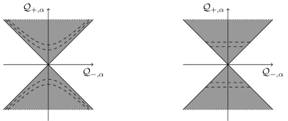
Figure 2: Motivation for the third reparametrization step. The dashed lines are the images of straight lines through the origin in $\mathfrak{a}^{+}$ before (left) and after (right) the reparametrization $R_{\rm III}$.

We are going to change the parametrization in such a way that the hyperbola is rectified to a straight line; see figure 2. Such a reparametrization gives us a handle on the boundary of the PS domain, as is discussed in the next subsection. Accordingly, the third reparametrization we use is given by

$$R_{\rm III}:\;\mathfrak{a}^{+}\times K\times_{Z_{K}(\mathfrak{a})}\mathcal{Q}_{+} \rightarrow\mathfrak{a}^{+}\times K\times_{Z_{K}(\mathfrak{a})}\mathcal{Q}_{+}\,,$$

$$(H,[k;X]) \mapsto\Big{(}H,\Big{[}k;X_{0}+\sum_{\alpha\in\Sigma_{+}(\mathcal{Q},\mathfrak{a})}\frac{1}{\cosh(\alpha(H))}X_{\alpha}\Big{]}\Big{)}.$$

This is another orientation preserving diffeomorphism. We thus obtain

$$PS\circ R_{\rm III}:\; \mathfrak{a}^{+}\times K\times_{Z_{K}(\mathfrak{a})}\mathcal{Q}_{+}\rightarrow\mathcal{Q},$$

$$(H, [k;X])\mapsto\operatorname{Ad}(k)\Big{(}X_{0}+\sum_{\mathclap{\alpha\in\Sigma_{+}(\mathcal{Q},\mathfrak{a})}}\big{(}X_{\alpha}+\tanh(\alpha(H))\phi(X_{\alpha})\big{)}\Big{)},$$ (13)

which is renamed to $PS$ in the following.

4.1.5 Reparametrization IV: Making the boundary visible

From the parametrization (13) (see also figure 2) it is clear that the boundary is reached when some $\alpha(H)$ goes to $\pm\infty$ and hence $\tanh$ goes to $\pm 1$. Put differently, the boundary of the domain of integration can be reached through a limit in the parameter space $\mathfrak{a}^{+}$. To obtain control over the boundary we have to make sense of the expression $\lim_{H\rightarrow\infty}\tanh(\alpha(H))$. This limit is encoded in the functions $T_{\alpha,c}$. Recall that

$$T_{\alpha,c}\left(\sum_{i\in I_{c}}h^{i}H_{i}\right)=\left\{\begin{array}[]{l l}\tanh\Big{(}\sum_{i\in I_{c}}\frac{h^{i}}{1-h^{i}}\alpha(H_{i})\Big{)},&\forall i:\,h^{i}<1\;\text{or}\;\alpha(H_{i})=0,\\ \operatorname{sgn}(\alpha(H_{i})),&\text{else},\end{array}\right.$$

where the index $c$ refers to the decomposition (8) of $\mathfrak{a}^{+}$ into the simplicial cones $\mathfrak{a}^{+}_{c}$. Fix $\alpha\in\Sigma_{+}(\mathcal{Q},\mathfrak{a})$ and $j\in I_{c}$ such that $\alpha(H_{j})\neq 0$. Then

$$\lim_{h^{j}\rightarrow 1}T_{\alpha,c}\left(\sum_{i\in I_{c}}h^{i}H_{i}\right)=\operatorname{sgn}(\alpha(H_{j})).$$

This shows that $T_{\alpha,c}$ is continuous. $T_{\alpha,c}$ is also differentiable since

$$\lim_{h^{j}\rightarrow 1}\partial_{h^{j}}\tanh\left(\sum_{i\in I_{c}}\frac{h^{i}}{1-h^{i}}\alpha(H_{i})\right)=0$$

generalizes to all higher (and mixed) partial derivatives.

To put the functions $T_{\alpha,c}$ to use we define for each cone $c\in C$ the mapping

$$R_{{\rm IV},c}:\;(\mathfrak{a}_{\emptyset,c}^{+})^{o}\times K\times_{Z_{K}(\mathfrak{a})}\mathcal{Q}_{+} \rightarrow\mathfrak{a}_{c}^{+}\times K\times_{Z_{K}(\mathfrak{a})}\mathcal{Q}_{+}\,,$$

$$\left(\sum_{i\in I_{c}}h^{i}H_{i},[k;X]\right) \mapsto\left(\sum_{i\in I_{c}}\frac{h^{i}}{1-h^{i}}H_{i},[k;X]\right),$$

where $(\mathfrak{a}_{\emptyset,c}^{+})^{o}$ denotes the interior of $\mathfrak{a}_{\emptyset,c}^{+}$. For each simplicial cone, this is an (orientation preserving) diffeomorphism onto its image. The mapping is visualized in figure 3. We use it to reparametrize $PS$ on each cone. We thus obtain $PS_{c}=PS\circ R_{{\rm IV},c}$ , which is the parametrization defined in lemma 4.1, eq. $\eqref{PS_c_parametrisation}$.

In the following we want to give the notion ‘boundary of the PS domain’ a precise meaning. In the case of integration cells, i.e., differentiable mappings defined on a cube, the boundary operator $\partial$ is defined as usual. $\partial$ can also be applied to integration chains, i.e. formal linear combinations of cells. In principle the correct procedure would be to decompose each $PS_{c}$ into cells in order to apply $\partial$. However, in the following we argue that we can treat each $PS_{c}$ effectively as single cell with the boundary operator $\partial$ acting just on the $\mathfrak{a}_{\emptyset,c}^{+}$ part of the domain of definition. Note that $\mathfrak{a}_{\emptyset,c}^{+}$ by the decomposition (9) is diffeomorphic to an $n$-dimensional cube.

First note that $PS_{c}$ extends as a differentiable mapping to a neighborhood of $\mathfrak{a}_{\emptyset,c}^{+}$ since the $T_{\alpha,c}$ are differentiable functions defined on $\mathfrak{a}$. Thus it is possible to define the orientation of the boundary. Furthermore, since $K$ is a closed compact manifold it suffices to discuss boundary contributions arising from a decomposition of $\mathcal{Q}_{+}$ into cells. By inspecting our parametrization we see that going to infinity on $\mathcal{Q}_{+}$ implies going to infinity in the domain of integration. In section 4.3 we show that the integrand goes to zero exponentially on this domain and hence all possible boundary contributions vanish. Thus we obtain part i) of lemma 4.1

Part ii) of lemma 4.1 follows immediately by noting that the mappings $R_{{\rm IV},c}$ are diffeomorphisms onto.

Since similar arguments are needed in several other parts of section 4, the proof of part iii) of lemma 4.1 is presented in appendix A.

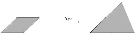
Figure 3: $\mathfrak{su}(2,2)$ example for $R_{\rm IV}$ mapping $\mathfrak{a}_{\emptyset}^{+}$ on the left hand side to $\mathfrak{a_{+}}$ on the right side. In this example there is only one simplicial cone.

4.2 Extending the PS domain

In this section we construct an extension of the PS domain which has no boundary other than the irrelevant boundary at infinity. The idea is to connect each boundary point to infinity by attaching one halfline. The directions of these halflines should be such that the attached domain does not contribute to the integral of $g(Q,A)\chi_{\epsilon}(Q)\,dQ$. We first determine such a direction for each boundary point, and then give a parametrization of the attached domains. In the following let

$$B(X,Y):=\operatorname{Tr}(XY)$$ (14)

denote the trace form on $\mathcal{Q}^{\mathbb{C}}$.

Some care must be exercised in order to guarantee the convergence of the integral on the extended PS domain. The positivity requirement $As>0$ in the theorem already gives a hint that the matrix $s$ plays a prominent role in the discussion of convergence. Owing to $s\in\mathcal{Q}_{+}$ we have the decomposition

$$s=s_{0}+\sum_{\mathclap{\alpha\in\Sigma_{+}(\mathcal{Q},\mathfrak{a})}}s_{\alpha}\,,$$ (15)

where $s_{0}\in\mathcal{Q}_{+,0}$ and $s_{\alpha}=\pi_{+,\alpha}(s)\in\mathcal{Q}_{+,\alpha}$.

The next lemma introduces the convergent directions which are used to extend $PS$ in such a way that convergence is maintained.

Lemma 4.2.

The matrices

$$E_{j}:=2\lim_{t\rightarrow\infty}\frac{\operatorname{Ad}(e^{tH_{j}})s}{\mathrm{max}_{\alpha\in\Sigma_{+}(\mathcal{Q},\mathfrak{a})}\;e^{|\alpha(tH_{j})|}}$$ (16)

are well defined and non-zero. The following properties hold for all $1\leq i,j\leq M$:

1. $\operatorname{Tr}(E_{i}\operatorname{Ad}(k)^{-1}A)>0$.

2. There exist numbers $e_{j}^{\alpha}\in\{0,1\}$ such that the matrices $E_{j}$ decompose as

   $$E_{j}=\sum_{\alpha(H_{j})\neq 0}e_{j}^{\alpha}\big{(}s_{\alpha}+\operatorname{sgn}(\alpha(H_{j}))\phi(s_{\alpha})\big{)}.$$ (17)

3. For $i,j\in I_{c}$ one has $B(E_{i},E_{j})=0$. In particular, $B(E_{i},E_{i})=0$.

Before we come to the proof of lemma 4.2, we formulate another lemma which suggests how to extend the PS domain. Note however that an integral over $PS$ needs a regulating function and that we postpone the discussion of convergence to section 4.3. Strictly speaking, the next lemma is not necessary for the proof of theorem 2.1. It is included as a preparation for the more involved definition of the homotopy introduced in section 4.3.

Lemma 4.3.

For $c\in C$ and $L\subset I_{c}$ the mappings

$$PS_{L,c}:\; \mathfrak{a}_{L,c}^{+}\times K\times_{Z_{K}(\mathfrak{a})}\mathcal{Q}_{+}\rightarrow\mathcal{Q}^{\mathbb{C}},$$

$$(H,[k; X])\mapsto\operatorname{Ad}(k)\Big{(}X_{0}+\sum_{\mathclap{\alpha\in\Sigma_{+}(\mathcal{Q},\mathfrak{a})}}\Big{(}X_{\alpha}+T_{\alpha,c}(H)\phi(X_{\alpha})\Big{)}-i\sum_{j\in L}(h^{j}-1)E_{j}\Big{)},$$

are well defined as integration chains and one has

$$\partial\left(\sum_{c\in C}\sum_{L\subset I_{c}}PS_{L,c}\right)=0,$$ (18)

as long as the sum of chains is integrated against forms with sufficiently rapid decay at infinity.

4.2.1 Proof of lemma 4.2

To see that the matrices $E_{i}$ are well defined, we express them in a more explicit fashion. A short calculation using (15) gives

$$\operatorname{Ad}(e^{H})s=s_{0}+\sum_{\mathclap{\alpha\in\Sigma_{+}(\mathcal{Q},\mathfrak{a})}}\big{(}\cosh(\alpha(H))s_{\alpha}+\sinh(\alpha(H))\phi(s_{\alpha})\big{)}.$$

This shows that the limit in (16) exists and that the matrices $E_{j}$ decompose as shown in equation (17). Thus we obtain $ii)$. Recalling that $\operatorname{ad}(s)|_{\mathfrak{p}}$ is injective we conclude that each of the matrices $E_{j}$ is non-zero.

For property $i)$ we note that $As>0$ and

$$s^{-1}E_{j}=2\lim_{t\rightarrow\infty}\frac{e^{-2tH_{j}}}{\mathrm{max}_{\alpha\in\Sigma_{+}(\mathcal{Q},\mathfrak{a})}\;e^{|\alpha(tH_{j})|}}\geq 0.$$

Thus $\operatorname{Tr}((\operatorname{Ad}(k)s^{-1}E_{j})As)$ is the trace of the product of the non-zero positive semidefinite hermitian matrix $s^{-1}\operatorname{Ad}(k)E_{j}$ and the positive hermitian matrix $As$. By inserting the eigenvalue representation $\sum_{n}p_{n}\pi_{n}$ of $s^{-1}\operatorname{Ad}(k)E_{j}$ we get

$$\operatorname{Tr}(s^{-1}\operatorname{Ad}(k)E_{j}As)=\sum_{n}p_{n}\operatorname{Tr}(\pi_{n}As).$$

Since $As$ is positive we have $\operatorname{Tr}(\pi_{n}As)>0$. Property $i)$ then follows because $s^{-1}\operatorname{Ad}(k)E_{j}\neq 0$ implies that there exists some $p_{n}>0$.

To prove property $iii)$ we use $ii)$ and note that for all $\alpha,\beta\in\Sigma_{+}(\mathcal{Q},\mathfrak{a})$ we have the orthogonality relations

$$B(s_{\alpha},s_{\beta})=-B(\phi(s_{\alpha}),\phi(s_{\beta}))=\delta_{\alpha,\beta}B(s_{\alpha},s_{\alpha})$$

and $B(s_{\alpha},\phi(s_{\beta}))=0$. We also recall that a fixed root $\alpha$ does not change sign on a fixed simplicial cone $\mathfrak{a}_{c}^{+}$. The desired result $B(E_{i},E_{j})=0$ for $i,j\in I_{c}$ then follows directly.

4.2.2 Proof of lemma 4.3

In this section we show that the mappings $PS_{L,c}$ in lemma 4.3 have the stated properties. First of all, the mappings are well defined since $Z_{K}(\mathfrak{a})$ acts trivially on the matrices $E_{i}$. We recall that the situation is visualized in figure 1.

$PS_{L,c}$ can be extended as a mapping to $\mathfrak{a}$ since $T_{\alpha,c}$ makes sense on $\mathfrak{a}$ and so does $(h^{j}-1)$. Thus $PS_{L,c}$ is well defined as an integration chain. By the same argument as for the $PS_{\emptyset,c}$ case, a boundary can arise only by the action of the boundary operator $\partial$ on the factor $\mathfrak{a}_{L,c}^{+}$.

In the following we always neglect possible boundary contributions from infinity, since the integrals under consideration are convergent by assumption.

To see that the different integration cells $PS_{L,c}$ and $PS_{L^{\prime},c^{\prime}}$ fit together in a seamless way, we recall that $\mathfrak{a}_{c}^{+}\cap\mathfrak{a}_{c^{\prime}}^{+}$ is again a simplicial cone which is generated by the set $\{H_{i}\}_{i\in I_{c}\cap I_{c^{\prime}}}$. In particular each $H\in\mathfrak{a}_{L,c}^{+}\cap\mathfrak{a}_{L^{\prime},c^{\prime}}^{+}$ can be represented in the form $H=\sum_{i\in I_{c}\cap I_{c^{\prime}}}h^{i}H_{i}$, which implies that $T_{\alpha,c}(H)=T_{\alpha,c^{\prime}}(H)$. We have $h^{i}\geq 1$ for $i\in L$ and $h^{i}\leq 1$ for $i\in I_{c}\setminus L$. Together with similar conditions from $L^{\prime}$ this yields

$$\sum_{i\in L}(h^{i}-1)E_{i}=\sum_{i\in L^{\prime}}(h^{i}-1)E_{i}$$

on the intersection $\mathfrak{a}_{L,c}^{+}\cap\mathfrak{a}_{L^{\prime},c^{\prime}}^{+}$. Hence we obtain the equality $PS_{L,c}(H,[k;X])=PS_{L^{\prime},c^{\prime}}(H,[k;X])$ on the joint domain of definition.

Moreover, the induced orientations on the boundaries between two neighboring cells are opposites of each other. Together with the fact (shown in appendix A) that the contributions from $\partial\mathfrak{a}^{+}$ are of codimension no less than two, these results yield (18).

To get some intuition for the situation it is useful to observe that the halflines which are glued to boundary points of the PS domain, point into directions within $\oplus_{\alpha\in\Sigma(\mathcal{Q},\mathfrak{a})}i\mathcal{Q}_{\alpha}$, and hence cannot coincide with vectors tangent to PS, which live in $\mathcal{Q}$.

4.3 Equivalence of $PS$ and $Euclid$

Finally, we show that the integral over $PS$ equals the integral over $Euclid$. The idea is to deform the extended PS domain into the subspace $\mathcal{Q}_{+}\oplus i[\mathfrak{p},s]$ of $\mathcal{Q}^{\mathbb{C}}$ where $B$ is positive. Recall that $[\mathfrak{p},s]=\mathcal{Q}_{-}$. We have to show that the integral remains convergent along the path of deformation and no boundary terms at infinity are generated. To that end we prefer to proceed in the reverse order and deform $Euclid$ into $PS$ to the extent that this is allowed by convergence of the integral. Recall that $Z_{K}(\mathfrak{a})$ acts trivially on $H_{i}\in\mathfrak{a}$ and the matrices $E_{i}$. It also acts trivially on $[H_{i},s]$ for all $i=1,\ldots,M$ because $k\in K$ is fixed by conjugation with $s$. For these reasons the mapping defined as

$$EPS_{L,c}^{\epsilon}:\,[\epsilon,1]\times \mathfrak{a}_{L,c}^{+}\times K\times_{Z_{K}(\mathfrak{a})}\mathcal{Q}_{+}\rightarrow\mathcal{Q}^{\mathbb{C}},$$

$$(t,H,[k;X])\mapsto \operatorname{Ad}(k)\Big{(}X_{0}+\sum_{\mathclap{\alpha\in\Sigma_{+}(\mathcal{Q},\mathfrak{a})}}\big{(}X_{\alpha}+(1-t)T_{\alpha,c}(H)\phi(X_{\alpha})\big{)}\Big{)}$$

$$-i\operatorname{Ad}(k)\sum_{j\in L}(h^{j}-1)\big{(}(1-t)E_{j}+2t[H_{j},s]\big{)}$$ (19)

is well defined. By reasoning similar to that for $PS_{L,c}$ each parametrization $EPS_{L,c}^{\epsilon}$ ($c\in C$) can be seen as an integration cell with boundary coming only from the $[\epsilon,1]\times\mathfrak{a}_{L,c}^{+}$ part. To simplify the notation we define

$$EPS^{\epsilon}:=\sum_{c\in C}\sum_{L\subset I_{c}}EPS_{L,c}^{\epsilon}\,,$$

$EPS_{L,c}:=EPS_{L,c}^{0}$ and similarly $EPS:=EPS^{0}$.

Lemma 4.4.

The mappings $EPS_{L,c}^{\epsilon}$ have the following properties:

1. The boundary of the sum $EPS^{\epsilon}$ is given by

   $$\partial(EPS^{\epsilon}) =Euclid-\sum_{c\in C}\sum_{L\subset I_{c}}EPS_{L,c}(t=\epsilon).$$

2. Let $g(Q,A):=e^{-\operatorname{Tr}(Q^{2})-2i\operatorname{Tr}(QA)}$. Then the integrals

   $$\int_{EPS_{L,c}(t=\epsilon)}g(Q,A)dQ$$

   exist for $\epsilon>0$.

3. For each $c\in C$ and $L\subset I_{c}$ with cardinality $|L|>0$ we have

   $$\lim_{\epsilon\rightarrow 0}\int_{EPS_{L,c}(\epsilon)}g(Q,A)dQ=0.$$

4. Let $PS(\epsilon):=\sum_{c\in C}EPS_{\emptyset,c}(\epsilon)$. The integral over $PS(\epsilon)$ in the limit $\epsilon\rightarrow 0$ may be computed as an integral over $PS$ with regularized integrand:

   $$\lim_{\epsilon\rightarrow 0}\int_{PS(\epsilon)}g(Q,A)dQ=\lim_{\epsilon\rightarrow 0}\int_{PS}g(Q,A)\chi_{\epsilon}(Q)dQ.$$

The proof of the lemma is spelled out in the next four subsections. Here we anticipate that once the lemma has been established, we can do the following series of manipulations:

$$\int_{Euclid}g(Q,A)dQ =\int_{Euclid}g(Q,A)dQ-\lim_{\epsilon\rightarrow 0}\int_{EPS^{\epsilon}}\underbrace{d(g(Q,A)dQ)}_{=0}\;,$$

$$\underset{i),ii)}{=}\lim_{\epsilon\rightarrow 0}\int_{EPS(\epsilon)}g(Q,A)dQ$$

$$\underset{ii),iii),iv)}{=}\lim_{\epsilon\rightarrow 0}\int_{PS(\epsilon)}g(Q,A)dQ$$

$$\underset{iv)}{=}\lim_{\epsilon\rightarrow 0}\int_{PS}g(Q,A)\chi_{\epsilon}(Q)dQ,$$

which yields the statement of our theorem 2.1.

4.3.1 Proof of $i)$: Deformation of $PS$ into $Euclid$

Next we prove statement $i)$ of lemma 4.4. By an argument similar to that in the proof of lemma 4.3 we obtain

$$\partial(EPS^{\epsilon})\equiv\sum_{c\in C}\sum_{L\subset I_{c}}\partial(EPS_{L,c}^{\epsilon})=EPS(t=1)-EPS(t=\epsilon).$$ (20)

We will now deal with the summand $EPS(1)$.

For $L\subsetneq I_{c}$ the mapping $EPS_{L,c}(t)$ degenerates in the limit $t\to 1$. More precisely, for $i\in I_{c}\setminus L$ we have $\partial_{h^{i}}EPS_{L,c}(1)=0$ and thus a reduction in dimension. Hence we have the following identity relating integration chains:

$$EPS(1)=\sum_{c\in C}EPS_{I_{c},c}(1).$$

In the following we establish the connection between $EPS(1)$ and $Euclid$. For $c\in C$ and $H=\sum_{i\in I_{c}}h^{i}H_{i}\in\mathfrak{a}_{I_{c},c}^{+}$ we have

$$EPS_{I_{c},c}(1,H,[k;X]) =\operatorname{Ad}(k)\Big{(}X-2i\sum_{j\in I_{c}}(h^{j}-1)[H_{j},s]\Big{)}.$$

To facilitate the interpretation of the expression on the right hand side, we now change the left factor of the domain of definition of $EPS_{I_{c},c}(1)$ from $\mathfrak{a}_{I_{c},c}^{+}$ to $\mathfrak{a}_{c}^{+}$. This is done by introducing the diffeomorphism

$$\psi_{c}:\;\mathfrak{a}_{I_{c},c}^{+} \rightarrow\mathfrak{a}_{c}^{+}\;,$$

$$H \mapsto\sum_{i\in I_{c}}(h^{i}-1)H_{i}\,.$$

By inserting it into the previous formula we get

$$EPS_{I_{c},c}(1,\psi_{c}^{-1}(H),[k;X]) =\operatorname{Ad}(k)\big{(}X-2i[H,s]\big{)}.$$

Note that while the composition with $\psi_{c}^{-1}$ does alter the mapping $EPS_{I_{c},c}(1)$, the effect is not a change of image but only a reparametrization.

The right hand side of the expression above does not have any explicit dependence on the simplicial cone $c$ any more. Therefore, by recalling $\bigcup_{c\in C}\mathfrak{a}_{c}^{+}=\mathfrak{a}^{+}$ and noting that the diffeomorphisms $\psi_{c}$ are orientation preserving, it is clear that our mappings $EPS_{I_{c},c}$ combine to a smooth mapping

$$\sum_{c\in C}EPS_{I_{c},c}(1)\circ(\psi_{c}^{-1},id):\quad \mathfrak{a}^{+}\times K\times_{Z_{K}(\mathfrak{a})}\mathcal{Q}_{+}\rightarrow\mathcal{Q}^{\mathbb{C}},$$

$$(H,[k;X])\mapsto\operatorname{Ad}(k)\big{(}X-2i[H,s]\big{)},$$

where $id$ stands for the identity on $K\times_{Z_{K}(\mathfrak{a})}\mathcal{Q}_{+}$.

The final step is to undo the reparametrizations $R_{\rm II}$ and $R_{\rm I}$ to obtain

$$\Big{(}\sum_{c\in C}EPS_{I_{c},c}(1)\circ(\psi_{c}^{-1},id)\Big{)}\circ R_{\rm II}^{-1}\circ R_{\rm I}^{-1}(Y,X)=X-2i[Y,s],$$

where $X\in\mathcal{Q}_{+}$ and $Y\in\mathfrak{p}$. Since $[\mathfrak{p},s]=\mathcal{Q}_{-}$ we conclude that $EPS(1)$ is the same as Euclid as an integration chain.

4.3.2 Proof of $ii)$: Existence of the integral for $\epsilon>0$

In this subsection we prove statement $ii)$ of lemma 4.4. Let us first make some general remarks and definitions which allow a simpler discussion of the integrals to be considered. For this purpose let $id_{L,c}$ be the identity on $\mathfrak{a}_{L,c}^{+}$ and recall that $R_{\rm II}$ yields a global factorization of the bundle $K\times_{Z_{K}(\mathfrak{a})}\mathcal{Q}_{+}$ as $K/Z_{K}(\mathfrak{a})\times\mathcal{Q}_{+}$. Let $d\mu([k])$ be a left invariant volume form on $K/Z_{K}(\mathfrak{a})$ and let $dH$ and $dQ_{+}$ denote constant volume forms on $\mathfrak{a}^{+}$ and $\mathcal{Q}_{+}$ respectively. Then there exist functions $P_{L,c}$ such that

$$\left(EPS_{L,c}(t=\epsilon)\circ(id_{L,c},R_{\rm II}^{-1})\right)^{*}dQ=P_{L,c}\;dH\wedge d\mu([k])\wedge dQ_{+}\,.$$

By inspection of $EPS_{L,c}$ and $R_{\rm II}^{-1}$ we see that $P_{L,c}$ depends polynomially on $\epsilon$, $[k]$, the matrix entries of $X\in\mathcal{Q}_{+}$, $h^{i}$, and on $\partial^{r}T_{\alpha,c}$, where $\partial^{r}$ represents any number of partial derivatives with respect to $h^{i}$. For the rest of the proof it is more convenient to switch to a formulation in terms of measures instead of volume forms. In that respect we have

$$\int_{\mathfrak{a}_{L,c}^{+}\times K/Z_{K}(\mathfrak{a})\times\mathcal{Q}_{+}}\Big{(}EPS_{L,c}(t=\epsilon)\circ(id_{L,c},R_{\rm II}^{-1})\Big{)}^{*}(g(\cdot,A)dQ)$$

$$= \int\limits_{\mathclap{\mathfrak{a}_{L,c}^{+}\times K/Z_{K}(\mathfrak{a})\times\mathcal{Q}_{+}}}g\Big{(}EPS_{L,c}(t=\epsilon)\circ(id_{L,c},R_{\rm II}^{-1}),A\Big{)}\;P_{L,c}\,|dH||d\mu([k])||dQ_{+}|,$$ (21)

where $|dH|$ and $|dQ_{+}|$ are Lebesgue measures on $\mathfrak{a}^{+}$ and on $\mathcal{Q}_{+}$ and $|d\mu([k])|$ denotes Haar measure on $K/Z_{K}(\mathfrak{a})$. To prove statement $ii)$ it is enough to show the existence of

$$\int_{K/Z_{K}(\mathfrak{a})}\int_{\mathfrak{a}_{L,c}^{+}}\int_{\mathcal{Q}_{+}}\Big{|}g\Big{(}EPS_{L,c}(t=\epsilon) \circ(id_{L,c},R_{\rm II}^{-1}),A\Big{)}\Big{|}$$ (22)

$$\times|P_{L,c}|\,|dQ_{+}||dH||d\mu([k])|.$$ (23)

Indeed, the Fubini-Tonelli theorem then asserts that the original integral exists and that Fubini’s theorem can be applied to (21).

We now deal with the integral (23). Note that replacing $K/Z_{K}(\mathfrak{a})$ by $K$ in (23) introduces only a constant factor which can be absorbed in the polynomial $P_{L,c}$. The mapping $R_{\rm II}^{-1}$ extends naturally from $K/Z_{K}(\mathfrak{a})\times\mathcal{Q}_{+}$ to $K\times\mathcal{Q}_{+}$ and, similarly, $EPS_{L,c}(t)$ extends from $\mathfrak{a}_{L,c}^{+}\times K\times_{Z_{K}(\mathfrak{a})}\mathcal{Q}_{+}$ to $\mathfrak{a}_{L,c}^{+}\times K\times\mathcal{Q}_{+}$. Furthermore we can apply for $k\in K$ the transformation

$$\mathcal{Q}_{+}\rightarrow\mathcal{Q}_{+}\,,\quad X\mapsto kXk^{-1},$$

in the inner integral over $\mathcal{Q}_{+}$. The corresponding Jacobian is unity. Hence (23) equals

$$\int\limits_{K}\int\limits_{\mathfrak{a}_{L,c}^{+}}\int\limits_{\mathclap{\mathcal{Q}_{+}}}\Big{|}g\Big{(}EPS_{L,c}(\epsilon),A\Big{)}\Big{|}\;|P_{L,c}|\,|dQ_{+}||dH||d\mu(k)|,$$ (24)

where $|d\mu(k)|$ is a Haar measure on $K$.

Let us now concentrate on the exponential function $g\big{(}EPS_{L,c}(\epsilon),A\big{)}$ which is responsible for the convergence of the integral. Referring to the second and third lines in (4.3), we define

$$\Xi :=\operatorname{Ad}(k)\Big{(}X_{0}+\sum_{\mathclap{\alpha\in\Sigma_{+}(\mathcal{Q},\mathfrak{a})}}\Big{(}X_{\alpha}+(1-\epsilon)T_{\alpha,c}(H)\phi(X_{\alpha})\Big{)}\Big{)},$$

$$\Upsilon :=-i\operatorname{Ad}(k)\sum_{j\in L}(h^{j}-1)\Big{(}(1-\epsilon)E_{j}+2\epsilon[H_{j},s]\Big{)},$$

which lets us write the integrand in the form

$$g\Big{(}EPS_{L,c}(\epsilon,H,k,X),A\Big{)}=e^{-B(\Xi+\Upsilon,\Xi+\Upsilon)-2iB(\Xi+\Upsilon,A)}.$$ (25)

Due to $A,\Xi\in\mathcal{Q}$ and $\Upsilon\in\mathrm{i}\mathcal{Q}$, the terms $B(\Xi,\Upsilon)$ and $iB(\Xi,A)$ are imaginary. Therefore, they do not contribute to (24). To evaluate the remaining terms we note some useful relations. For $X_{\alpha}\in\mathcal{Q}_{+,\alpha}$ and $X,X^{\prime}\in\bigoplus_{\alpha\in\Sigma_{+}(\mathcal{Q},\mathfrak{a})}\mathcal{Q}_{+,\alpha}$ we have

$$B(X_{\alpha},X_{\beta})=\delta_{\alpha,\beta}B(X_{\alpha},X_{\alpha}),$$ (26)

$$B(X,X^{\prime})=-B(\phi(X),\phi(X^{\prime})),\quad B(\phi(X),X^{\prime})=0.$$ (27)

$B(\Xi,\Xi)$ can be re-expressed as

$$B(\Xi,\Xi) \underset{\mathclap{\eqref{orth_1}}}{=}\operatorname{Tr}(X_{0}^{2})+\sum_{\mathclap{\alpha\in\Sigma_{+}(\mathcal{Q},\mathfrak{a})}}\operatorname{Tr}\big{(}X_{\alpha}+(1-\epsilon)T_{\alpha,c}(H)\phi(X_{\alpha})\big{)}^{2}$$

$$\underset{\mathclap{\eqref{orth_2}}}{=}B(X_{0},X_{0})+\sum_{\mathclap{\alpha\in\Sigma_{+}(\mathcal{Q},\mathfrak{a})}}B(X_{\alpha},X_{\alpha})\Big{(}1-(1-\epsilon)^{2}T_{\alpha,c}^{2}(H)\Big{)}.$$ (28)

$B$ is positive on $\mathcal{Q}_{+}$, and for all $H\in\mathfrak{a}^{+}$ and $0<\epsilon<1$ we have

$$0<\epsilon(2-\epsilon)\leq 1-(1-\epsilon)^{2}T_{\alpha,c}^{2}(H)\leq 1.$$ (29)

Thus $B(\Xi,\Xi)$ is positive definite. Since all dependence on $X\in\mathcal{Q}_{+}$ occurs in $B(\Xi,\Xi)$ this guarantees the convergence of the inner integral in (24) for $\epsilon>0$.

We turn to $B(\Upsilon,\Upsilon)$. Statement $iii)$ of lemma 4.2 asserts that $B(E_{i},E_{j})=0$ for $i,j\in L\subset I_{c}$. Hence we have

$$B(\Upsilon,\Upsilon)=B(\Upsilon_{0},\Upsilon_{0})+4\epsilon(1-\epsilon)\sum_{i,j\in L}(h^{i}-1)(h^{j}-1)B(-[H_{j},s],E_{i}),$$

where $\Upsilon_{0}=-2i\epsilon\mathrm{Ad}(k)\sum_{j}(h^{j}-1)[H_{j},s]$. Note that $B(\Upsilon_{0},\Upsilon_{0})\geq 0$ since $\Upsilon_{0}\in i\mathcal{Q}_{-}$. The remaining terms of $B(\Upsilon,\Upsilon)$ are non-negative since

$$B(-[H_{j},s],E_{i}) \underset{\mathclap{\eqref{s_decomposition}}}{=}B\Big{(}-\sum_{\mathclap{\alpha\in\Sigma_{+}(\mathcal{Q},\mathfrak{a})}}\alpha(H_{j})\phi(s_{\alpha}),E_{i}\Big{)}$$

$$\underset{\mathclap{\eqref{E_{i,c}_explicit_decomposition}}}{=}\;\;-\sum_{\mathclap{\alpha,\beta\in\Sigma_{+}(\mathcal{Q},\mathfrak{a})}}e_{i}^{\beta}\operatorname{sgn}(\beta(H_{i}))\alpha(H_{j})B(\phi(s_{\alpha}),\phi(s_{\beta}))$$

$$=\;\;-\sum_{\mathclap{\alpha\in\Sigma_{+}(\mathcal{Q},\mathfrak{a})}}e_{i}^{\alpha}|\alpha(H_{j})|B(\phi(s_{\alpha}),\phi(s_{\alpha}))\geq 0.$$

Since $E_{i}$ is non-zero, identity $\eqref{E_{i,c}_explicit_decomposition}$ ensures that there exists some $\alpha\in\Sigma_{+}(\mathcal{Q},\mathfrak{a})$ such that $e_{i}^{\alpha}\neq 0$, $\alpha(H_{i})\neq 0$ and $s_{\alpha}\neq 0$. Thus we have

$$B(-[H_{i},s],E_{i})>0.$$

Together with (29) this shows that the second (or middle) integral in (24) exists. This conclusion is not changed by the factor $e^{-2iB(\Upsilon,A})$ as $B(\Upsilon,A)$ is linear in the variables $h^{j}$ whereas $B(\Upsilon,\Upsilon)$ is quadratic. The result depends continuously on $k\in K$ and we hence conclude that the outer integral over the compact group $K$ exists. It follows that all integrals $\int_{EPS_{L,c}(\epsilon)}g(\cdot,A)dQ$ exist for $\epsilon>0$.

4.3.3 Proof of $iii)$: The limit $\mathbf{\lim_{\epsilon\rightarrow 0}}$

Recall from section 4.3.2 that Fubini’s theorem applies to the integral (21). We repeat the steps which led to (24) except that now we do not take the absolute value of the integrand. Thus we obtain

$$\int\limits_{\mathclap{EPS_{L,c}(\epsilon)}}g(Q,A)\,dQ=\int_{K}\int_{\mathfrak{a}_{L,c}^{+}}\int_{\mathcal{Q}_{+}}g(EPS_{L,c}(\epsilon),A)\,P_{L,c}\,|dQ_{+}||dH||d\mu(k)|.$$ (30)

The reason why statement $iii)$ of lemma 4.4 holds true is a very general one: the convergence of the integral to zero is brought about by cancelations due to an oscillatory term. More specifically, by integrating along one special direction in $\mathcal{Q}_{+}$ we obtain essentially a regularized delta distribution. Our parametrization is well suited to exhibit this mechanism explicitly. We will show that it is possible to perform the limit $\epsilon\rightarrow 0$ after doing the inner Gaussian integrations.

In the following, Einstein’s summation convention is in place. We can choose a basis of $\mathcal{Q}_{+}$ with coordinates $x^{l}$ such that the quadratic form $Q\mapsto\operatorname{Tr}Q^{2}$ is diagonal. The choice of basis will be made explicit below. Schematically speaking, the Gaussian integrations over $\mathcal{Q}_{+}$ in (30) are of the form

$$I_{L,c,\epsilon}(H,k):=e^{-h^{i}\tilde{g}_{i}}\int\limits_{\mathbb{R}^{\mathrm{dim}\,\mathcal{Q}_{+}}}e^{-(x^{l})^{2}f_{l}-2ix^{l}g_{l}}P_{L,c}\prod_{l}dx^{l},$$

where $\tilde{g}_{i}(\epsilon,k)$, $f_{l}(\epsilon,h^{i},k)$ and $g_{l}(\epsilon,h^{i},k)$ are functions of $k\in K$, $\epsilon\in[0,1]$ and $H\in\mathfrak{a}_{L,c}^{+}$. These functions will be specified as we go along. Now it is possible to introduce sources $j_{l}$ for $x^{l}$ and perform the integral:

$$I_{L,c,\epsilon}(H,k) =e^{-h^{i}\tilde{g}_{i}}P_{L,c}^{\prime}(\partial_{j_{l}},\dots)\int e^{-f_{l}(x^{l})^{2}-2ix^{l}(g_{l}+j_{l})}\prod_{l}dx^{l}\Big{|}_{j_{l=0}}$$

$$=e^{-h^{i}\tilde{g}_{i}}P_{L,c}^{\prime}(\partial_{j_{l}},\dots)\prod_{l}\sqrt{\frac{\pi}{f_{l}}}e^{-\frac{(g_{l}+j_{l})^{2}}{f_{l}}}\Big{|}_{j_{l=0}}$$

$$=e^{-h^{i}\tilde{g}_{i}}P_{L,c}^{\prime\prime}(\frac{1}{f_{l}},g_{l},\dots)\prod_{l}\sqrt{\frac{\pi}{f_{l}}}e^{-\frac{g_{l}^{2}}{f_{l}}},$$ (31)

where primes just indicate that these are different polynomials, and the dots represent a dependence on $\epsilon$, $h^{i}$, $k$ and $\partial^{r}T_{\alpha,c}$. Assuming that $|L|>0$, we will show that for $\epsilon\rightarrow 0$ we have $f_{1}\rightarrow 0$ and $g_{1}\neq 0$ for a suitable choice of basis of $\mathcal{Q}_{+}$. We also show that $f_{l}\geq 0$ and $g_{l}\in\mathbb{R}$ for all $l$ and $\epsilon\in[0,1]$. The exponential then dominates the polynomial and (31) converges to zero in the limit of $\epsilon\rightarrow 0$. In addition, we show that $\tilde{g}_{i}>0$, which has the consequence that the remaining integrals over $\mathfrak{a}_{L,c}^{+}$ are convergent (since $h^{i}>0$).

Thus the issue of convergence is reduced to a discussion of the functions $\tilde{g}_{i}$, $f_{l}$ and $g_{l}$. We start with $\tilde{g}_{i}$. Reading it off from its definition by

$$2iB(\Upsilon,A)=(h^{i}-1)\tilde{g}_{i},$$

we find that it has the expression

$$\tilde{g}_{i}=2B(\operatorname{Ad}(k)((1-\epsilon)E_{i}+2\epsilon[H_{i},s]),A).$$

From inequality i) of lemma 4.2 we infer that $2B(\mathrm{Ad}(k)E_{i},A)\geq c>0$, since $k\in K$ and $K$ is compact. (Recall that $A$ is fixed.) We thus see that $\tilde{g}_{i}>0$ for small enough $\epsilon$.

To discuss the functions $f_{l}$ and $g_{l}$ we have to choose a basis of $\mathcal{Q}_{+}$. For this purpose we fix some $j\in L$, recalling that $L\not=\emptyset$ in the situation at hand. We then consider the decomposition

$$\mathcal{Q}_{+}=\mathcal{Q}_{+,0}\oplus\bigoplus_{\alpha(H_{j})\neq 0}\mathcal{Q}_{+,\alpha}\oplus\bigoplus_{\alpha(H_{j})=0}\mathcal{Q}_{+,\alpha}\,.$$ (32)

We define $m:=\text{dim}\oplus_{\alpha(H_{j})\neq 0}\mathcal{Q}_{+,\alpha}$ and $m^{\prime}:=\text{dim}\oplus_{\alpha(H_{j})=0}\mathcal{Q}_{+,\alpha}$. Denoting by $\Pi_{\mathcal{Q}_{+}}$ the orthogonal projection onto $\mathcal{Q}_{+}$ we introduce

$$X_{1}:=\Pi_{\mathcal{Q}_{+}}(E_{j})=\sum_{\mathclap{\alpha(H_{j})\neq 0}}e_{j}^{\alpha}s_{\alpha}\not=0.$$

We extend $X_{1}$ to an orthogonal basis $\{X_{l}\}_{l=1,\ldots,m}$ of $\oplus_{\alpha(H_{j})\neq 0}\mathcal{Q}_{+,\alpha}$. We also fix an orthogonal basis $\{X_{l}\}_{l=m+1,\ldots,m+m^{\prime}}$ of $\oplus_{\alpha(H_{j})=0}\mathcal{Q}_{+,\alpha}$ which respects the root decomposition. For the basis vectors $\{X_{l}\}_{l=1,\ldots,m+m^{\prime}}$ we have identities like those in (26) and (27).

Recall that on $\mathfrak{a}_{L,c}^{+}$ we have $h^{j}\geq 1$ and therefore $|T_{\alpha,c}(H)|=1$ if $\alpha(H_{j})\not=0$. As is shown by

$$B(\Xi,\Xi)\underset{\eqref{B_Xi_Xi}}{=}B(X_{0},X_{0}) +(1-(1-\epsilon)^{2})\sum_{\mathclap{\alpha(H_{j})\neq 0}}B(X_{\alpha},X_{\alpha})$$

$$+\sum_{\mathclap{\alpha(H_{j})=0}}\Big{(}1-(1-\epsilon)^{2}T_{\alpha,c}^{2}(H)\Big{)}B(X_{\alpha},X_{\alpha})$$

$$=B(X_{0},X_{0}) +\sum_{l=1}^{m+m^{\prime}}(x^{l})^{2}f_{l}\,,$$ (33)

our choice of basis diagonalizes the quadratic form $B(\Xi,\Xi)$. We also see that $f_{l}\geq 0$. In particular, for $l=1$ we have

$$f_{1}=\epsilon(2-\epsilon)B(X_{1},X_{1}).$$

Note that $f_{1}\to 0$ for $\epsilon\to 0$.

It is easy to check that the coefficients $g_{l}$ defined by

$$-2iB(\Xi,A)-2B(\Xi,\Upsilon)=-2ix^{l}g_{l}$$ (34)

are real. By using the statements $ii)$ and $i)$ of lemma 4.2 we have

$$\lim_{\epsilon\rightarrow 0}\;{g}_{1}=B(E_{j},\operatorname{Ad}(k^{-1})A)>0.$$

Thus we obtain the result

$$\lim_{\epsilon\rightarrow 0}\int_{\mathcal{Q}_{+}}g(EPS_{L,c}(\epsilon),A)\,P_{L,c}\,|dQ_{+}|=0.$$ (35)

Since the dependence on $H\in\mathfrak{a}_{L,c}^{+}$ in (35) is governed by the exponential function $\exp(-h^{i}\tilde{g}_{i})$ with $\tilde{g}_{i}>0$ and the dependence on $k\in K$ is continuous, the limit $\epsilon\rightarrow 0$ is uniform. Thus, taking the limit commutes with the outer integrals and we obtain the third part of lemma 4.4.

4.3.4 Proof of $iv)$: Reaching $PS$

It remains to prove statement iv) of lemma 4.4. To that end, for any $c\in C$ we introduce on $\mathfrak{a}_{\emptyset,c}^{+}\times K$ the two functions

$$I_{c,\epsilon} :=\int\limits_{\mathcal{Q}_{+}}g(EPS_{\emptyset,c}(\epsilon),A)P_{\emptyset,c}|dQ_{+}|,$$ (36)

$$I_{c,\epsilon}^{\prime} :=\int\limits_{\mathcal{Q}_{+}}g(PS_{\emptyset,c},A)\chi_{\epsilon}(PS_{\emptyset,c})P_{\emptyset,c}(\epsilon=0,\cdot)d|Q_{+}|.$$ (37)

To prove the desired statement, it is sufficient to show that

$$\lim_{\epsilon\rightarrow 0}\int\limits_{K}\int\limits_{\mathfrak{a}_{\emptyset,c}^{+}}I_{c,\epsilon}|dH||d\mu(k)| =\lim_{\epsilon\rightarrow 0}\int\limits_{K}\int\limits_{\mathfrak{a}_{\emptyset,c}^{+}}I_{c,\epsilon}^{\prime}|dH||d\mu(k)|$$ (38)

holds for all $c\in C$. We will do so by using Lebesgue’s dominated convergence theorem on both sides of (38).

Let us first establish that the two functions defined in (37) converge pointwise to the same function in the limit of $\epsilon\rightarrow 0$. For that, we have to distinguish between two situations for $H\in\mathfrak{a}_{\emptyset,c}^{+}$: there either exists a non-trivial $L\subset I_{c}$ such that $H\in\mathfrak{a}_{L,c}^{+}\cap\mathfrak{a}_{\emptyset,c}^{+}$, or there does not. In the first situation we can apply the result of the previous section to see that $\lim_{\epsilon\rightarrow 0}I_{c,\epsilon}(H,k)=0$ for all $k\in K$. A similar argument yields the same result for the function $I_{c,\epsilon}^{\prime}$. In the second situation there are no problems of convergence with the $\mathcal{Q}_{+}$-integral (see (28)) and we can directly set $\epsilon=0$, in which case the two functions coincide by definition. Thus we always have $I_{c,0}=I_{c,0}^{\prime}$.

From now on, for brevity, we discuss only the left hand side of (38), as the discussion of the right hand side is completely analogous. Our strategy is to show that the function $(\epsilon,H,k)\mapsto I_{c,\epsilon}(H,k)$ on the compact domain $[0,1]\times\mathfrak{a}_{\emptyset,c}^{+}\times K$ is continuous and hence integrable. The property of continuity on a compact domain implies that the function $I_{c,\epsilon}$ is dominated by a constant function, which in turn is integrable as well. Thus we will be able to draw the desired conclusion by applying Lebesgue’s dominated convergence theorem.

Following the line of reasoning of the last subsection we choose for $\mathcal{Q}_{+}$ an orthogonal basis $\{X_{l}^{\prime}\}_{l=1,\ldots,\mathrm{dim}\mathcal{Q}_{+}}$ compatible with the decomposition $\oplus_{\alpha}\mathcal{Q}_{+,\alpha}$. This means that for each $l$ there exists a unique root $\alpha_{l}$ (possibly the zero root) such that $X_{l}\in\mathcal{Q}_{+,\alpha_{l}}$. Moreover, whenever a root $\alpha$ is such that $s$ has non-zero projection $s_{\alpha}=\pi_{+,\alpha}(s)$, then we take $s_{\alpha}\in\mathcal{Q}_{+,\alpha}$ to be an element of our basis set $\{X_{l}^{\prime}\}$. We arrange for these non-zero vectors $s_{\alpha}$ to be the first $m_{1}$ vectors of the set $\{X_{l}^{\prime}\}$.

By adaptation (due to the change of basis $\{X_{l}\}\to\{X_{l}^{\prime}\}$) of the definitions (33) and (34) we obtain new coefficient functions

$$f_{l}^{\prime} =\left(1-(1-\epsilon)^{2}T_{\alpha_{l},c}^{2}\right)B(X_{l}^{\prime},X_{l}^{\prime}),$$

$$g_{l}^{\prime} =\operatorname{Tr}\left(\big{(}X_{l}^{\prime}+(1-\epsilon)T_{\alpha_{l},c}\,\phi(X_{l}^{\prime})\big{)}k^{-1}Ak\right),$$

superseding the earlier functions $f_{l}$ and $g_{l}$. If $\alpha_{l}$ is the zero root we set $T_{0,c}=0$. Note that $g_{l}^{\prime}$ is still real and $f_{l}^{\prime}\geq 0$. By recalling the dependence on $H\in\mathfrak{a}_{\emptyset,c}^{+}$ of the functions $T_{\alpha,c}$ defined in section 4.1, we see that if $\epsilon\rightarrow 0$ and if $h^{j}\rightarrow 1$ for at least one index $j\in I_{c}$, then we have $f_{l}^{\prime}\to 0$ for all $l$ with $\alpha_{l}(H_{j})\neq 0$. In view of this behavior, the set of problematic points where continuity of the function $(\epsilon,H,k)\mapsto I_{c,\epsilon}(H,k)$ is not obvious is the set

$$\{0\}\times\Big{\{}\sum_{i\in I_{c}}h^{i}H_{i}\in\mathfrak{a}_{\emptyset,c}^{+}\mid\exists i\in I_{c}:h^{i}=1\Big{\}}\times K,$$ (39)

as will be clear presently. To be precise, the limit function $I_{c,0}$ is not even defined on this set. Our main work in the rest of this subsection will be to show that it extends continuously as zero. We will do so by constructing a continuous function which dominates $|I_{c,\epsilon}|$ and is zero at the problematic points.

In the following we restrict the discussion to the case of only one summand of the polynomial in (31). Its modulus is certainly smaller than

$$C\,\prod_{l}\frac{\exp(-g_{l}^{\prime 2}/f_{l}^{\prime})}{f_{l}^{\prime n_{l}/2}},$$

with a constant $C>0$ and natural numbers $n_{l}$. Here we have dropped the factors corresponding to zero roots, as these are of no relevance for our present purpose. Fixing some regular element $\tilde{H}\in\mathfrak{a}_{\emptyset,c}^{+}$, so that $\alpha(\tilde{H})\neq 0$ for all $\alpha\in\Sigma_{+}(\mathcal{Q},\mathfrak{a})$, we introduce the functions

$$g_{l}^{\prime\prime}:=\operatorname{Tr}\left(\big{(}X_{l}^{\prime}+\operatorname{sgn}(\alpha_{l}(\tilde{H}))\phi(X_{l}^{\prime})\big{)}k^{-1}Ak\right).$$

By a short computation, these have the convenient property that

$$\frac{g_{l}^{\prime 2}-g_{l}^{\prime\prime 2}}{f_{l}}= -\left(\operatorname{Tr}\phi(X_{l}^{\prime})k^{-1}Ak\right)^{2}-2\frac{\operatorname{Tr}(X_{l}^{\prime}k^{-1}Ak)\operatorname{Tr}\left(\phi(X_{l}^{\prime})k^{-1}Ak\right)}{\operatorname{sgn}(\alpha_{l}(\tilde{H}))(1+(1-\epsilon)|T_{\alpha_{l},c}|)}$$

is a continuous function on the compact space $[0,1]\times\mathfrak{a}_{\emptyset,c}^{+}\times K$ and there exists a constant $C^{\prime}>0$ for which we have the upper bound

$$C\,\prod_{l}\frac{\exp(-g_{l}^{\prime 2}/f_{l}^{\prime})}{f_{l}^{\prime n_{l}/2}}<C^{\prime}\,\prod_{l}\frac{\exp\left(-g_{l}^{\prime\prime 2}/f_{l}^{\prime}\right)}{f_{l}^{\prime n_{l}/2}}.$$ (40)

For the next step, we recall the constancy on $\mathfrak{a}_{\emptyset,c}^{+}$ of the sign function $\operatorname{sgn}(\alpha(\tilde{H}))=\operatorname{sgn}(\alpha_{l}(H_{j}))$ for $\alpha_{l}(H_{j})\not=0$. By parts $i)$ and $ii)$ of lemma 4.2 and our choice of basis elements $X_{l}^{\prime}=s_{\alpha_{l}}$ for $l=1,\ldots,m_{1}$ we then have

$$\sum_{l\leq m_{1}\text{ and }\alpha_{l}(H_{j})\neq 0}e_{j}^{\alpha_{l}}g_{l}^{\prime\prime}=\operatorname{Tr}(E_{j}k^{-1}Ak)>0$$ (41)

for every $j\in I_{c}$. For the following discussion we let $k\in K$ be arbitrary but fixed. Inequality (41) guarantees that there exists a neighborhood $U_{k}$ of $k$ so that for each $j\in\{1,\ldots,\text{dim}\,\mathfrak{a}\}$ there exists an $l_{j}\in\{1,\ldots,\text{dim}\mathcal{Q}_{+}\}$ with the property that $g_{l_{j}}^{\prime\prime}>0$ on $U_{k}$. By inspection of the right hand side of (40) one can see that its behavior (in the limit $\epsilon\to 0$ and close to the set of problematic points) is very similar to that of $\exp(-1/x)/x^{a}$ for $x\rightarrow 0$ and positive exponent $a$. To make this observation more tangible we now show how to simplify the dependence of $f_{l}^{\prime}$ on $H\in\mathfrak{a}_{\emptyset,c}^{+}$. As a first step, we note that only the first factor on the right hand side of

$$f_{l}^{\prime}=(1-(1-\epsilon)|T_{\alpha_{l},c}|)(1+(1-\epsilon)|T_{\alpha_{l},c}|)B(X_{l}^{\prime},X_{l}^{\prime})$$

is relevant for the discussion of the limit behavior. Now let $H_{1},H_{2}\in\mathfrak{a}_{\emptyset,c}^{+}$ and write $T_{j}\equiv|T_{\alpha_{l},c}(H_{j})|$ and $b_{l}\equiv B(X_{l}^{\prime},X_{l}^{\prime})$ for short. By invoking the addition formula for the hyperbolic tangent,

$$\tanh(x+y)=\frac{\tanh(x)+\tanh(y)}{1+\tanh(x)\tanh(y)},$$

and observing that this formula carries over to our functions $T_{\alpha,c}$, we obtain

$$1-(1-\epsilon)|T_{\alpha_{l},c}(H_{1}+H_{2})|=\frac{(1-(1-\epsilon)T_{1})(1-(1-\epsilon)T_{2})+\epsilon(2-\epsilon)T_{1}T_{2}}{1+T_{1}T_{2}}\,.$$ (42)

We claim that this identity yields the following bounds:

$$\frac{1}{2}\prod_{i=1,2}(1-(1-\epsilon)T_{i})\leq b_{l}^{-1}f_{l}^{\prime}(\epsilon,H_{1}+H_{2})\leq 6\prod_{i=1,2}\sqrt{1-(1-\epsilon)T_{i}}\,,$$ (43)

of which the left one is immediate. To verify the right inequality we observe that, by the identity preceding it, a stronger statement is

$$(1-(1-\epsilon)T_{1})(1-(1-\epsilon)T_{2})+\epsilon(2-\epsilon)T_{1}T_{2}\leq 3\prod_{i=1,2}\sqrt{1-(1-\epsilon)T_{i}}\,.$$

Owing to $0\leq T_{i}\leq 1$ this inequality is obviously true if $\epsilon=0$. So let $0<\epsilon\leq 1$. Then the two square root factors on the right hand side never vanish and we may divide by them. Since the resulting first term on the left hand side is never greater than one, the remaining job is to show that

$$\frac{\epsilon(2-\epsilon)T_{1}T_{2}}{\sqrt{1-(1-\epsilon)T_{1}}\sqrt{1-(1-\epsilon)T_{2}}}\leq 2.$$ (44)

This follows from $T_{1}T_{2}\leq 1$ and $\sqrt{1-(1-\epsilon)T_{1}}\sqrt{1-(1-\epsilon)T_{2}}\geq\epsilon$, which concludes our proof of (43). As an easy consequence of (43) we have

$$\frac{1}{8b_{l}}f_{l}^{\prime}(H_{1})f_{l}^{\prime}(H_{2})\leq f_{l}^{\prime}(H_{1}+H_{2})\leq 6\sqrt{f_{l}^{\prime}(H_{1})f_{l}^{\prime}(H_{2})}.$$

We now use these bounds to simplify the dependence on $H=\sum h^{i}H_{i}\in\mathfrak{a}_{\emptyset,c}^{+}$ on the right hand side of (40). Iteration gives

$$\frac{\exp\left(-g_{l}^{\prime\prime 2}/f_{l}^{\prime}\right)}{f_{l}^{\prime n_{l}/2}}\leq\frac{\exp(-\tilde{C}g_{l}^{\prime\prime 2}/\prod_{i\in I_{c}}(1-(1-\epsilon)|T_{\alpha_{l},c}(h^{i}H_{i})|)^{n_{i,c}})}{\prod_{i\in I_{c}}(1-(1-\epsilon)|T_{\alpha_{l},c}(h^{i}H_{i})|)^{n_{i,c}^{\prime}}}.$$ (45)

On the right hand side $h^{i}\alpha_{l}(H_{i})$ is meant without summation convention and $\tilde{C},n_{i,c}$ and $n_{i,c}^{\prime}$ are positive constants. By (16) and (17) it follows that $|\alpha_{l_{j}}(H_{j})|=\text{max}_{\alpha}|\alpha(H_{j})|$. This property can be used to see that (45) is bounded by

$$\frac{\exp(-\tilde{C}g_{l}^{\prime\prime 2}/\prod_{i\in I_{c}}(1-(1-\epsilon)|T_{\alpha_{l},c}(h^{i}H_{i})|)^{n_{i,c}})}{\prod_{i\in I_{c}}(1-(1-\epsilon)|T_{\alpha_{l_{i}},c}(h^{i}H_{i})|)^{n_{i,c}^{\prime}}}.$$

The exponential part of the right hand side is continuous and hence we have the bound

$$C\,\prod_{l=1}^{\text{dim}\mathcal{Q}_{+}}\frac{\exp(-g_{l}^{\prime 2}/f_{l}^{\prime})}{f_{l}^{\prime n_{l}/2}}<\tilde{C}^{\prime}\prod_{i=1}^{\text{dim}\mathfrak{a}}\frac{\exp(-\tilde{C}g_{l_{i}}^{\prime\prime 2}/(1-(1-\epsilon)|T_{\alpha_{l_{i}},c}(h^{i}H_{i})|)^{n_{i,c}})}{(1-(1-\epsilon)|T_{\alpha_{l_{i}},c}(h^{i}H_{i})|)^{m_{i,c}^{\prime}}}$$

where $\tilde{C}^{\prime}$ and $m_{i,c}^{\prime}$ are positive constants. Now it is easy to see that the right hand side is essentially a product of continuous functions of the form $\exp(-c/x^{a})/x^{b}$ (with $a,b,c>0$) which are composed with continuous functions of the form $(1-(1-\epsilon)|T_{\alpha_{l_{i}},c}(h^{i}H_{i})|)$. Thus we obtain a dominating function for $I_{c,\epsilon}$ on a neighborhood of $k$. In particular this yields continuity of $I_{c,\epsilon}$ in each point of the set $\{0\}\times\{\sum_{i\in I_{c}}h^{i}H_{i}\in\mathfrak{a}_{\emptyset,c}^{+}\mid\exists i\in I_{c}:h^{i}=1\}\times\{k\}$. Since $k$ was taken to be arbitrary we obtain that $I_{c,\epsilon}$ is a continuous function on $[0,1]\times\mathfrak{a}_{\emptyset,c}^{+}\times K$. Thus $I_{c,\epsilon}$ attains a maximum. The maximum is a dominating function and hence Lebesgue’s dominated convergence theorem can be applied. This finishes the proof of statement $iv)$ in lemma 4.4, which was the last step needed to complete the proof of Theorem 2.1 .

Remark 4.1.

To obtain the theorem when $\mathfrak{g}=\mathfrak{k}\oplus\mathfrak{p}$ is the direct sum of an Abelian and a semisimple Lie algebra, let $\mathfrak{a}^{\prime}\oplus\mathfrak{a}$ denote the corresponding decomposition of a maximal Abelian subalgebra of $\mathfrak{p}$ and replace $\mathfrak{a}^{+}$ by $\mathfrak{a}^{\prime}\times\mathfrak{a}^{+}$ and $H$ by $H^{\prime}+H$ everywhere in the proof. In addition let $\tilde{\mathfrak{k}}$ denote the semisimple part of $\mathfrak{k}$ and replace $\mathfrak{k}$ by $\tilde{\mathfrak{k}}$ everywhere in the proof.

Remark 4.2.

It is possible to choose different regularization functions $\chi_{\epsilon}$. The choice made here seems natural, as it has the highest invariance possible and was also used in earlier work.

Remark 4.3.

The convergence properties can be seen quite clearly in the discussion of $I_{c,\epsilon}(\epsilon,H,[k])$. The convergence is not uniform in $A$. To have uniform convergence, we need $As\geq\delta>0$. In applications with $As\geq 0$, one has to replace $A$ by $A+\delta s$. For fixed $\delta>0$ this gives uniform convergence in $A$.

4.4 Different representations of the integral, and alternating signs

In this section we establish two different representations of the integral over the PS domain. These are stated in corollaries 2.1 and 2.2.

Recall that the ‘Jacobian’ $J^{\prime}(\lambda)$ which appears in both representations may have alternating sign. In the following proof of corollary 2.1 we pinpoint the origin of these surprising signs. First we review the setting. Recall that the elements of $\mathfrak{k}$ are antihermitian and those of $\mathcal{Q}_{+}$ hermitian. Since $\tilde{\mathfrak{g}}=\mathfrak{k}\oplus\mathcal{Q}_{+}$ is closed under hermitian conjugation, it is the direct sum of an Abelian and a semisimple Lie algebra. The semisimple part of $\tilde{\mathfrak{g}}$ is denoted by $\tilde{\mathfrak{g}}_{s}$. We choose a maximal Abelian subalgebra $\mathfrak{h}$ of $\mathcal{Q}_{+}$ containing $s$. The decomposition of $\tilde{\mathfrak{g}}$ into an Abelian and a semisimple part induces a decomposition of $\mathfrak{h}=\mathfrak{h}_{a}\oplus\mathfrak{h}_{s}$ and $\mathfrak{k}=\mathfrak{k}_{a}\oplus\mathfrak{k}_{s}$. Here $\mathfrak{h}_{a}$ and $\mathfrak{k}_{a}$ lie in the Abelian part of $\tilde{\mathfrak{g}}$ while $\mathfrak{h}_{s}$ and $\mathfrak{k}_{s}$ lie in the semisimple part of $\tilde{\mathfrak{g}}$. Let $(\mathfrak{h}_{s}^{+})^{o}$ denote a positive open Weyl chamber in $\mathfrak{h}_{s}$ with respect to the semisimple Lie algebra $\tilde{\mathfrak{g}}_{s}$. We also define $K_{s}=\exp{\mathfrak{k}_{s}}$. Then we have the following reparametrization:

$$\tilde{R}:\;\mathfrak{p}\times K_{s}/Z_{K_{s}}(\mathfrak{h}_{s})\times(\mathfrak{h}_{s}^{+})^{o}\times\mathfrak{h}_{a} \rightarrow\mathfrak{p}\oplus\mathcal{Q}_{+}\,,$$

$$(Y,[k],H_{s},H_{a}) \mapsto(Y,k(H_{s}+H_{a})k^{-1}).$$

Recall that $K=\exp\mathfrak{k}$ is closed by assumption and $G$ denotes the closed and analytic subgroup of $GL(n,\mathbb{C})$ with Lie algebra $\mathfrak{g}=\mathfrak{k}\oplus\mathfrak{p}$. The subgroup $K_{a}=\exp\mathfrak{k}_{a}\subset K$ is central and closed. By the diffeomorphism $\mathfrak{p}\to\exp{\mathfrak{p}}$ and the isomorphism $K_{s}/Z_{K_{s}}(\mathfrak{h}_{s})\cong K/(K_{a}Z_{K_{s}}(\mathfrak{h}_{s}))$ we have the reparametrization

$$R:\;\exp(\mathfrak{p})K/(K_{a}Z_{K_{s}}(\mathfrak{h}_{s}))\times(\mathfrak{h}_{s}^{+})^{o}\times\mathfrak{h}_{a} \rightarrow\mathfrak{p}\oplus\mathcal{Q}_{+}\,,$$

$$(e^{Y}[k],H_{s},H_{a}) \mapsto(Y,k(H_{s}+H_{a})k^{-1}).$$

By $K_{a}Z_{K_{s}}(\mathfrak{h}_{s})=Z_{K}(\mathfrak{h}_{s})$ and the Cartan decomposition $G=\exp(\mathfrak{p})K$ (see [11]) we obtain yet another parametrization of the PS domain,

$$PS\circ R:\;G/Z_{K}(\mathfrak{h}_{s})\times(\mathfrak{h}_{s}^{+})^{o}\times\mathfrak{h}_{a} \rightarrow\mathcal{Q},$$

$$([g],H_{s},H_{a}) \mapsto g(H_{s}+H_{a})g^{-1},$$

which is the one most frequently used in the literature.

To proceed with the proof of corollary 2.1, we have to diagonalize the commutator action of $\mathfrak{h}$ on $\tilde{\mathfrak{g}}$ and on $\mathfrak{p}\oplus\mathcal{Q}_{-}$. For this purpose we note that the values $\alpha(H_{s}+H_{a})$ of the roots $\alpha$ are real since $[H_{s}+H_{a},\cdot]$ is hermitian with respect to the hermitian form $\operatorname{Tr}(X^{\dagger}Y)$. Moreover $\alpha(H_{a})=0$ for $\alpha\in\Sigma_{+}(\mathfrak{k}\oplus\mathcal{Q}_{+},\mathfrak{h})$.

The pullback of $dQ$ by $PS\circ R$ is then

$$(PS \circ R)^{*}dQ=\Delta(H_{s}+H_{a})\,d\mu([g])\wedge dH,$$

where $d\mu([g])$ is a left invariant volume form on $G/Z_{K}(\mathfrak{h}_{s})$ and $dH$ is a constant volume form on $\mathfrak{h}$. Denoting by $d_{\alpha}$ the dimension of the root space corresponding to $\alpha$, we get

$$\Delta(H_{s}+H_{a})=\prod_{\alpha\in\Sigma_{+}(\mathfrak{k}\oplus\mathcal{Q}_{+},\mathfrak{h})}\alpha(H_{s})^{d_{\alpha}}\prod_{\beta\in\Sigma_{+}(\mathfrak{p}\oplus\mathcal{Q}_{-},\mathfrak{h})}\beta(H_{s}+H_{a})^{d_{\beta}}.$$

Note that $\Delta$ differs from $J^{\prime}$ in corollary 2.1 only by taking the modulus of the roots in $\Sigma_{+}(\mathfrak{k}\oplus\mathcal{Q}_{+},\mathfrak{h})$. But these roots $\alpha\in\Sigma_{+}(\mathfrak{k}\oplus\mathcal{Q}_{+},\mathfrak{h})$ are positive when evaluated on $(\mathfrak{h}_{s}^{+})^{o}$. Therefore we have the following equality:

$$\int_{PS\circ R}f(Q)\,dQ=\int_{id}f(g(H_{s}+H_{a})g^{-1})J^{\prime}(H_{s}+H_{a})\,d\mu([g])\wedge dH,$$

where $id$ denotes the identity on $G/Z_{K}(\mathfrak{h}_{s})\times(\mathfrak{h}_{s}^{+})^{o}\times\mathfrak{h}_{a}$.

At this point a crucial difference between the roots in $\Sigma_{+}(\mathfrak{k}\oplus\mathcal{Q}_{+},\mathfrak{h})$ and those in $\Sigma_{+}(\mathfrak{p}\oplus\mathcal{Q}_{-},\mathfrak{h})$ is detected: since the definition of the Weyl chamber $\mathfrak{h}_{+}^{o}$ refers only to the former roots, it is possible for the latter roots to change sign on $\mathfrak{h}_{+}^{o}$. These sign changes are particulary evident in our approach as we are integrating differential forms instead of densities (or measures).

Now it is convenient to replace the volume form $d\mu([g])$ by the left invariant measure $|d\mu([g])|$ and $dH$ by Lebesgue measure $|dH|$ on $\mathfrak{h}:$

$$\int\limits_{\mathclap{PS\circ R}}f(Q)\,dQ=\quad\int\limits_{\mathclap{G/Z_{K}(\mathfrak{h}_{s})\times(\mathfrak{h}_{s}^{+})^{o}\times\mathfrak{h}_{a}}}f(g(H_{s}+H_{a})g^{-1})J^{\prime}(H_{s}+H_{a})|d\mu([g])||dH|.$$

The replacement of $G/(K_{a}Z_{K_{s}}(\mathfrak{h}_{s}))$ by $G$ simply leads to a change of normalization constant $c^{\prime}\in\mathbb{R}\setminus\{0\}$:

$$\int\limits_{\mathclap{PS\circ R}}f(Q)\,dQ=c^{\prime}\int\limits_{\mathclap{G\times(\mathfrak{h}_{s}^{+})^{o}\times\mathfrak{h}_{a}}}f(g(H_{s}+H_{a})g^{-1})J^{\prime}(H_{s}+H_{a})|d\mu(g)||dH|,$$

where $|d\mu(g)|$ denotes Haar measure on $G$.

Let $N_{K_{s}}(\mathfrak{h}_{s})$ denote the normalizer of $\exp\mathfrak{h}_{s}$ in $K_{s}$. In the following we make use of the Weyl group $N_{K_{s}}(\mathfrak{h}_{s})/Z_{K_{s}}(\mathfrak{h}_{s})$. This Weyl group acts on $\mathfrak{h}_{s}$ and generates $\mathfrak{h}_{s}$ from $\mathfrak{h}_{s}^{+}$. To exploit this property we need that $J^{\prime}$ is invariant under the action of the Weyl group. Recall that $J^{\prime}$ is given by

$$J^{\prime}(H)=\prod_{\alpha\in\Sigma_{+}(\mathfrak{k}\oplus\mathcal{Q}_{+},\mathfrak{h})}|\alpha(H)^{d_{\alpha}}|\prod_{\beta\in\Sigma_{+}(\mathfrak{p}\oplus\mathcal{Q}_{-},\mathfrak{h})}\beta(H)^{d_{\beta}}.$$

The first factor is trivially invariant, whereas for the second factor an additional argument is needed. For that purpose we define a root $\beta\in\Sigma(\mathfrak{p}\oplus\mathcal{Q}_{-},\mathfrak{h})$ to be positive if $\beta(s)>0$. This definition makes sense because $\beta(s)\neq 0$ for all roots $\beta\in\Sigma(\mathfrak{p}\oplus\mathcal{Q}_{-},\mathfrak{h})$. Since $s$ is $\operatorname{Ad}(K)$ invariant we conclude that the action of the Weyl group does no more than permute the roots in $\Sigma_{+}(\mathfrak{p}\oplus\mathcal{Q}_{-},\mathfrak{h})$. Hence $\Sigma_{+}(\mathfrak{p}\oplus\mathcal{Q}_{-},\mathfrak{h})$ is Weyl-invariant and so is $J^{\prime}$. Now the Haar measure $|d\mu(g)|$ is $G$-bi-invariant and hence Weyl-invariant. Therefore, introducing another normalization constant $c^{\prime\prime}\in\mathbb{R}\setminus\{0\}$ we have

$$\int\limits_{\mathclap{PS\circ R}}f(Q)\,dQ=c^{\prime\prime}\int\limits_{\mathclap{G\times\mathfrak{h}}}f(gHg^{-1})J^{\prime}(H)|d\mu(g)||dH|.$$

By setting $f=g\cdot\chi_{\epsilon}$ we obtain corollary 2.1.

Since $PS$ is nearly everywhere injective and regular by assumption, so is $PS\circ R$. Application of the change of variable theorem then yields corollary 2.2.

Appendix A Contributions from $\partial\mathfrak{a}^{+}$

Here we give the detailed argument showing that for our purpose of integrating over $PS$ and $EPS^{\epsilon}$ the contributions from the boundary $\partial\mathfrak{a}^{+}$ of the Weyl chamber $\mathfrak{a}^{+}$ are irrelevant, as they are of codimension at least two.

Without loss, we fix any $c\in C$ and let $H_{i}\in\mathfrak{a}^{+}_{c}\cap\partial\mathfrak{a}^{+}$ be any one of the generators of $\mathfrak{a}_{c}^{+}$ which also lie in $\partial\mathfrak{a}^{+}$ (if there is no such generator then there is nothing to prove). By removing this generator we get a boundary component

$$\mathfrak{a}_{i,c}^{+}:=\mathfrak{a}_{i,c}\cap\mathfrak{a}^{+}\subset\partial\mathfrak{a}_{c}^{+}\cap\partial\mathfrak{a}^{+}\;,\quad\mathfrak{a}_{i,c}:=\left\{\sum\nolimits_{j\in I_{c}\setminus\{i\}}h^{j}H_{j}\mid h^{j}\in\mathbb{R}\right\}.$$

Next recall the definition of $PS_{c}$ in (10). We now show that by restricting to $\mathfrak{a}_{i,c}^{+}$ in the leftmost factor of the domain of definition of $PS_{c}$ we get a domain of codimension at least two. Here the main observation is that the dimension of the isotropy group of $\mathfrak{a}$ changes at the boundary of $\mathfrak{a}^{+}$ and, in particular, $\dim Z_{K}(\mathfrak{a}_{i,c})>\dim Z_{K}(\mathfrak{a})$. This is seen as follows. Each face of $\partial\mathfrak{a}^{+}$ lies in the zero locus $\mathrm{ker}\,\alpha$ of some root $\alpha\in\Sigma(\mathfrak{g},\mathfrak{a})$ and we can arrange for $\mathfrak{a}_{i,c}\subset\mathrm{ker}\,\alpha$. If $\mathfrak{g}_{\alpha}$ is the root space of $\alpha$, the group generated by $\operatorname{Fix}_{\theta}(\mathfrak{g}_{\alpha}\oplus\mathfrak{g}_{-\alpha})\not\subset\mathrm{Lie}Z_{K}(\mathfrak{a})$ leaves the face $\mathfrak{a}_{i,c}^{+}$ invariant. When restricting $PS\circ R_{\rm I}$ in the first factor to $\mathfrak{a}_{i,c}^{+}$ we may replace the second factor $K/Z_{K}(\mathfrak{a})$ by the lower dimensional space $K/Z_{K}(\mathfrak{a}_{i,c})$ without changing the image of the parametrization. Thus the reduction $\mathrm{dim}\,\mathfrak{a}_{i,c}^{+}<\mathrm{dim}\,\mathfrak{a}$ is accompanied by a reduction of dimension of the $K$-orbits on $H\in\mathfrak{a}_{i,c}^{+}$. Altogether, the dimension is reduced by no less than two. Moreover, the eigenspace decomposition of $\mathcal{Q}$ with respect to $\mathfrak{a}$ is a refinement of the eigenspace decomposition w.r.t. the smaller abelian algebra $\mathfrak{a}_{i,c}$. Hence our further reparametrizations of PS (by $R_{\rm III}$ and $R_{\rm IV}$, which rely on an eigenspace decomposition of $\mathcal{Q}$) are compatible with the restriction of $\mathfrak{a}$ to $\mathfrak{a}_{i,c}$. This completes the argument for $PS_{c}$.

Turning to $EPS^{\epsilon}$, we have to argue that the analogous restriction is still well defined. For that, it is enough to note that for $X\in Z_{K}(\mathfrak{a}_{i,c})$ we have $[X,E_{j}]=0$ if $j\neq i$. By this token we see that also for $EPS^{\epsilon}$ the contributions from $\partial\mathfrak{a}^{+}$ are of codimension at least two.

Appendix B Equivalence of $SW$ and $Euclid$

A detailed discussion of the SW domain and the validity of the pertinent Hubbard-Stratonovich transformation can be found in [14]. Here we give another proof by deforming $SW$ into $Euclid$. By using some of the constructions of the proof for the PS domain, this deformation can be stated very explicitly.

We start with a brief discussion of the convergence of the Gaussian integral (1) over

$$SW:\;\mathfrak{p}\oplus\mathcal{Q}_{+} \rightarrow\mathcal{Q}^{\mathbb{C}},$$

$$(Y,X) \mapsto X-ibe^{Y}se^{-Y}.$$

For $X\in\mathcal{Q}_{+}$ and $Y\in\mathfrak{p}$ we have that $B(X,X)\geq 0$ and

$$B(ibe^{Y}se^{-Y},ibe^{Y}se^{-Y})=-b^{2}B(s,s)$$

is constant. The cross term $B(X,ibe^{Y}se^{-Y})$ is purely imaginary, and

$$-iB(-ibe^{Y}se^{-Y},A)=-b\operatorname{Tr}(e^{-2Y}As)<0$$

for $b>0$ yields convergence in the $\mathfrak{p}$ directions.

To see the properties of $SW$ more explicitly, we use the reparametrization $R_{\rm I}$ and the decomposition of $s$ to obtain

$$SW\circ R_{\rm I}:\;\mathfrak{a}^{+}\times K/Z_{K}(\mathfrak{a})\times Q_{+}\rightarrow\mathcal{Q}^{\mathbb{C}},$$

$$(H,[k],X)\mapsto X-ib\operatorname{Ad}(k)\Big{(}s_{0}+\sum_{\mathclap{\alpha\in\Sigma_{+}(\mathcal{Q},\mathfrak{a})}}\big{(}\cosh(\alpha(H))s_{\alpha}+\sinh(\alpha(H))\phi(s_{\alpha})\big{)}\Big{)}.$$

From this parametrization we see that the image of the boundary of $\mathfrak{a}^{+}$ is again of codimension at least two, which clearly shows that $\partial(SW)=0$.

A homotopy from $SW$ to $Euclid$ is given by

$$ESW:\;[0,1] \times\mathfrak{a}^{+}\times K/Z_{K}(\mathfrak{a})\times\mathcal{Q}_{+}\rightarrow\mathcal{Q}^{\mathbb{C}},$$

$$(t,H,[k],X) \mapsto X-ib\operatorname{Ad}(k)\Big{[}(1-t)s_{0}+$$

$$\sum_{\mathclap{\alpha\in\Sigma_{+}(\mathcal{Q},\mathfrak{a})}} [(\cosh((1-t)\alpha(H))-t)s_{\alpha}+\frac{\sinh((1-t)\alpha(H))}{1-t}\,\phi(s_{\alpha})]\,\Big{]}.$$

Note that $ESW(t=0)=SW$ and $ESW(t=1,H,[k],X)=X-ib[kHk^{-1},s]$. Since $[\mathfrak{p},s]=\mathcal{Q}_{-}$ we obtain $ESW(1)=Euclid$.

To complete the argument we show that the integral over $ESW$ is convergent. For this we note that for $Q_{t}=ESW(t,H,[k],X)$ we have

$$B(Q_{t},Q_{t})=B(X,X)+\sum_{\mathclap{\alpha\in\Sigma_{+}(\mathcal{Q},\mathfrak{a})}}(2t-t^{2})\frac{\sinh^{2}((1-t)\alpha(H))}{(1-t)^{2}}B(s_{\alpha},s_{\alpha})+\dots\;,$$

where the dots represent unimportant terms; these are terms which are purely imaginary, terms which are linear in $\sinh$ and all terms containing $s_{0}$. Owing to $B(X,X)\geq 0$ and $B(s_{\alpha},s_{\alpha})>0$ we obtain convergence for $t>0$. For $t=0$ convergence is ensured by the $B(Q,A)$ term, as was discussed above for the $SW$ parametrization.

Acknowledgment. This research was financially supported by a grant from the Deutsche Forschungsgemeinschaft (SFB/TR 12). J.M.H. gratefully acknowledges useful discussions with P. Heinzner.

References

• [1] F. Wegner, The mobility edge problem: continuous symmetry and a conjecture, Z. Phys. B 36, 207 (1979).
• [2] L. Schäfer and F. Wegner, Disordered systems with n orbitals per site: Lagrange formulation, hyperbolic symmetry, and Goldstone modes, Z. Phys. B 38, 113 (1980).
• [3] A.M.M. Pruisken and L. Schäfer, The Anderson model for electron localization nonlinear sigma model, asymptotic gauge invariance, Nucl. Phys. B 200, 20 (1982).
• [4] K.B. Efetov, Supersymmetry and the theory of disordered metals, Adv. Phys. 32, 53 (1983).
• [5] K.B. Efetov, Supersymmetry and the theory of disordered metals (Cambridge University Press, Cambridge, 1997).
• [6] M.R. Zirnbauer, Supersymmetry methods in random matrix theory, Encyclop. of Math. Phys. vol. 5, p.151-160 (Elsevier, Amsterdam, 2006).
• [7] Y.V. Fyodorov, On Hubbard-Stratonovich transformations over hyperbolic domains, J. Phys.: Condensed Matter 17, S1915 (2005).
• [8] Y. Wei and Y.V. Fyodorov, A conjecture on Hubbard-Stratonovich transformations for the Pruisken-Schäfer parametrizations of real hyperbolic domains, J. Phys. A 40, 13587 (2007).
• [9] Y.V. Fyodorov, Y. Wei, and M.R. Zirnbauer, Hyperbolic Hubbard-Stratonovich transformation made rigorous, J. Math. Phys. 9, 53507 (2008).
• [10] J.J.M. Verbaarschot, H.A. Weidenmüller, and M.R. Zirnbauer, Grassmann integration in stochastic quantum physics - the case of compound nucleus scattering, Phys. Rep. 129, 367 (1985).
• [11] A.W. Knapp, Lie Groups Beyond an Introduction (Birkhäuser, Boston, 2005, second edition, third printing).
• [12] G.M. Ziegler, Lectures on Polytopes (Springer-Verlag, New York, 1994).
• [13] J.A. De Loera, J. Rambau and F. Santos, Triangulations (Spinger-Verlag, Berlin, 2010).
• [14] M.R. Zirnbauer, Riemannian symmetric superspaces and their origin in random-matrix theory, J. Math. Phys. 37, 4986 (1996).