Model Selection by Loss Rank for Classification and Unsupervised Learning
 

Abstract

Hutter (2007) recently introduced the loss rank principle (LoRP) as a general-purpose principle for model selection. The LoRP enjoys many attractive properties and deserves further investigations. The LoRP has been well-studied for regression framework in Hutter and Tran (2010). In this paper, we study the LoRP for classification framework, and develop it further for model selection problems in unsupervised learning where the main interest is to describe the associations between input measurements, like cluster analysis or graphical modelling. Theoretical properties and simulation studies are presented.

Keywords

Classification, graphical models, loss rank principle, model selection.

1 Introduction

Model selection. Model selection is an important problem in machine learning and statistics. Typically, model selection can be regarded as the question of choosing the right model complexity. The maximum likelihood principle (MLP) breaks down when one has to select among a set of nested models, because then the MLP always selects the biggest model (w.r.t. inclusion). Overfitting is a serious problem in structural learning from data. Much effort has been put into developing model selection criteria that can avoid overfitting. The most popular ones are probably AIC (Akaike, 1973), the BIC (Schwarz, 1978), the $C_{p}$ (Mallows, 1973), the MDL (Rissanen, 1978), cross-validation (Allen, 1974; Craven and Wahba, 1979) and criteria based on Rademacher complexities (Koltchinskii, 2001; Bartlett et al., 2002). The reader is referred to Shao (1996); Hutter and Tran (2010) for comparisons of/some of these criteria. The loss rank principle (LoRP) introduced recently in Hutter (2007); Hutter and Tran (2010) is another contribution to the model selection literature. The LoRP, as it is named, is a general-purpose principle for model selection rather than a specific criterion. The LoRP can be regarded as a guiding principle for deriving model selection criteria that can avoid overfitting. It has the advantage of always giving answers, even in cases where the other criteria can not be used.

The loss rank principle. Consider the problem of selecting a model among a given set of models ${\cal M}$ achieving some kind of optimality properties. The main goal of the LoRP is to establish a selection criterion that is able to specify a parsimonious model that fits the data not too bad. General speaking, the LoRP consists in the so-called loss rank of a model defined as the number of other (fictitious) data that fit the model better than the actual data, and the model selected is the one with the smallest loss rank.

We now briefly present the LoRP developed in Hutter (2007) and Hutter and Tran (2010) for supervised learning settings. In supervised learning, the data is categorized into input and output, and the main interest is to develop a model for predicting output based on input. Let $D=(\boldsymbol{x},\boldsymbol{y})=\{(x_{1},y_{1}),...,(x_{n},y_{n})\}\in({\cal X}\times{\cal Y})^{n}$ be the (actual) training data set with $\boldsymbol{x}=(x_{1},...,x_{n})$ are inputs and $\boldsymbol{y}=(y_{1},...,y_{n})$ are (disturbed) outputs. Suppose that we use a model $M\in{\cal M}$ to fit the data $D$, e.g., $M$ is a linear regression model with $d$ covariates, or $M$ is a $k$-nearest neighbors regression model. Imagine that in experiment situations we can conduct the experiment many times with fixed design points $\boldsymbol{x}$. We then would get many other (fictitious) outputs $\boldsymbol{y}^{\prime}$. Let $\text{\rm Loss}_{M}(\boldsymbol{y}|\boldsymbol{x})$ be the empirical loss associated with a certain loss function when using a model $M\in{\cal M}$ to fit the data set $(\boldsymbol{x},\boldsymbol{y})$. For instance, $\text{\rm Loss}_{M}(\boldsymbol{y}|\boldsymbol{x})$ can be the least squares error, or the negative maximum log-likelihood when a sampling distribution is assumed. The loss rank of model $M$ then is defined as

$$\text{\rm LR}(M|D):=\mu\left\{\boldsymbol{y}^{\prime}\in{\cal Y}^{n}:\text{\rm Loss}_{M}(\boldsymbol{y}^{\prime}|\boldsymbol{x})\leq\text{\rm Loss}_{M}(\boldsymbol{y}|\boldsymbol{x})\right\}$$ (1)

with some measure $\mu$ on ${\cal Y}^{n}$. For example, $\mu$ can be the counting measure if ${\cal Y}$ is discrete, the usual Lebesgue measure on $I\mskip-3.0mu\mskip-3.0muR^{n}$ if ${\cal Y}=I\mskip-3.0mu\mskip-3.0muR$, or some empirical probability measure (see Sections below). Intuitively, the loss rank is large for too flexible models fitting $D=(\boldsymbol{x},\boldsymbol{y})$ well and also for too rigid models that fit $D$ not well (in both cases the model fits many other $D^{\prime}=(\boldsymbol{x},\boldsymbol{y}^{\prime})$ better). For example, consider the polynomial regression problem where $(x_{i},y_{i})\in I\mskip-3.0mu\mskip-3.0muR^{2}$, a higher order polynomial would fit $D$ well and also fit many other data $D^{\prime}$ well, thus resulting in a large loss rank. It was argued in Hutter (2007) and Hutter and Tran (2010) that minimizing the loss rank is a suitable model selection criterion which trades off the quality of fit with the model flexibility.

The LoRP has been well studied for regression with continuous response (Hutter and Tran, 2010). With continuous data and under squared loss, the loss rank has a closed form and many optimality properties of the LoRP have been pointed out. For example, the LoRP (i) is model selection consistent in some special cases; (ii) reduces to Bayesian model selection in linear basis function regression with Gaussian prior; (iii) has a minimum description length interpretation (interested readers are referred to Hutter and Tran (2010) for the details). Furthermore, the LoRP in supervised learning settings has been proven efficient in some specific applications. Tran (2009) demonstrated the use of LoRP for selecting the ridge parameter in ridge regression, while it was shown in Tran (2010) that shrinkage parameters in regularization procedures like Lasso (Tibshirani, 1996) or SCAD (Fan and Li, 2001) selected by the LoRP enjoy good statistical properties.

The LoRP seems to be a promising principle with a lot of potential, leading to a rich field. We would like to emphasize that the LoRP should be regarded as a guiding principle which in specific applications helps to derive model selection criteria that can avoid overfitting. This paper continues our investigation of the LoRP as a general-purpose procedure for model selection. We first study the LoRP for classification framework where the response is discrete. Based on the LoRP, we derive a model selection criterion for classification and show that minimizing the criterion is asymptotically equivalent to minimizing an ideal criterion which is only known when the population distribution is known.

Second, we develop the LoRP for model selection in unsupervised learning settings. This unsupervised learning LoRP then is studied by means of simulation in two specific applications: selection of number of clusters in cluster analysis and model selection in graphical modelling. The simulation shows that the model selection criteria derived from the LoRP work well and are competitive to existing ones.

We end this introduction section by listing some attractive properties of the LoRP. The LoRP

• always gives answers;

• does not require insight into the inner structure of the problem;

• does not require any explicit setting of the stochastic noise structure, i.e. no assumption of sampling distribution is needed;

• would work with any loss function.

2 Model Selection by Loss Rank for Classification

We consider in this section the model selection problem in a (binary) classification framework. Let $D=\{(X_{1},Y_{1}),...,(X_{n},Y_{n})\}$ be $n$ independent realizations of random variables $(X,Y)$, where $X$ takes on values in some space ${\cal X}$ and $Y$ is a $\{0,1\}$-valued random variable. We assume that these pairs are defined on a probability space $(\Omega,\Sigma,{\rm P})$ with $\Omega=({\cal X}\times{\cal Y})^{n}$. We are interested in constructing a predictor $t:{\cal X}\to\{0,1\}$ that predicts $Y$ based on $X$. The performance of the predictor $t$ is ideally measured by the prediction loss

$${\rm P}\gamma(t)={\rm P}(I_{Y\not=t(X)})={\rm P}(Y\not=t(X))$$ (2)

where $\gamma(t)(x,y):=I_{y\not=t(x)}$ is called the contrast function. Hereafter, for a measure $\mu$ and a $\mu$-integrable function $f$, we denote the integral $\int fd\mu$ by $\mu f$ or $\mu(f)$.

Ideally, we want to seek an optimal predictor $s$ that minimizes ${\rm P}\gamma(t)$ over all measurable $t:{\cal X}\to\{0,1\}$. However, finding such a predictor is impossible in practice because the class of all measurable functions $t:{\cal X}\to\{0,1\}$ is huge and typically not specified. Instead, we may restrict to some small class of predictors ${\cal F}$. A question arises immediately here: how small should the class ${\cal F}$ be? A too small ${\cal F}$ may lead to an unreasonable prediction loss, while finding an optimizer in a too large ${\cal F}$ may be an impossible task. Therefore the class/model ${\cal F}$ itself must be selected as well (the terms class and model will be used interchangeably). In this paper, we are interested in the model selection problem in which we would like to find a good model (in a sense specified later on) in a given set of models $\{{\cal F}_{m},\ m\in{\cal M}\}$.

The unknown prediction loss (2) is often estimated by the empirical risk

$${\rm P}_{n}\gamma(t)={\textstyle{1\over n}}\sum_{1}^{n}I_{Y_{i}\not=t(X_{i})}$$ (3)

where ${\rm P}_{n}$ is the empirical measure based on data $D$

$${\rm P}_{n}={\textstyle{1\over n}}\sum_{1}^{n}\delta_{(X_{i},Y_{i})}$$

with $\delta_{x}$ denotes the Dirac measure at $x$. For a class ${\cal F}_{m}$, one may seek a function $\hat{t}_{m}$ minimizing ${\rm P}_{n}\gamma(t)$ over $t\in{\cal F}_{m}$. Unfortunately, it is well-known that such a method leads to overfitting: the larger ${\cal F}_{m}$, the smaller the empirical risk ${\rm P}_{n}\gamma(\hat{t}_{m})$. Consequently, the selected model is always the biggest one. This leads to the idea of accounting for the model complexity, in which we select a model $\hat{m}$ that minimizes the sum of the empirical risk and a penalty term taking the model complexity into account.

Because ${\rm P}_{n}\gamma(t)$ underestimates ${\rm P}\gamma(t)$, a well-known regularized criterion for model selection is to penalize the approximation on ${\cal F}_{m}$ of the prediction loss by the empirical risk (see, e.g., Koltchinskii (2001); Fromont (2007); Arlot (2008))

$$\text{\rm crit}_{n}(m)={\rm P}_{n}\gamma(\hat{t}_{m})+\sup_{t\in{\cal F}_{m}}({\rm P}-{\rm P}_{n})\gamma(t).$$ (4)

The second term, denoted by $\text{\rm pen}_{n}(m)$, is a natural measure of the complexity of class ${\cal F}_{m}$, which measures the accuracy of empirical approximation on class ${\cal F}_{m}$. Then, the model to be selected is $m_{n}=\text{\rm arg}\min_{m}\{\text{\rm crit}_{n}(m)\}$. For simplicity, we assume throughout the paper that $m_{n}$ is uniquely determined.

In practice, ${\rm P}$ is unknown and so is $\text{\rm pen}_{n}(m)$. One has to estimate $\text{\rm pen}_{n}(m)$. Many methods have been proposed to estimate this theoretical penalty: VC-dimension (Vapnik and Chervonenkis, 1971), Rademacher complexities (Koltchinskii, 2001; Bartlett et al., 2002), resampling penalties (Fromont, 2007; Arlot, 2008). All of these methods give upper bounds for $\text{\rm pen}_{n}(m)$. The performances of the methods are measured in terms of oracle inequalities. The sharper the estimate is, the better the performance is. These methods often works well in practice but are not without problems. For example, the VC-dimension is often unknown and needs to be estimated by another upper bound, Rademacher complexities are often criticized to be too large (the local Rademacher complexities (Bartlett et al., 2005; Koltchinskii, 2006) have been introduced to overcome this drawback, however the latter still suffer from the hard-calibration problem because they involve unknown constants).

In this section, based on the LoRP, we propose a criterion to estimate the model $m_{n}$ directly, not $\text{\rm pen}_{n}$. Instead of giving an upper bound for $\text{\rm pen}_{n}(m)$, we directly estimate $m_{n}$ by minimizing a criterion over models $m\in{\cal M}$. Minimizing the criterion is asymptotically equivalent to minimizing $\text{\rm crit}_{n}(m)$ with probability 1 (Theorem 1).

In Section 2.1, the suggested criterion is derived and its model consistency is proven. In Section 2.2, we discuss the implementation and carry out a numerical example to demonstrate the criterion and compare it to other methods.

2.1 The loss rank criterion

The LoRP, as it is named, is a guiding principle rather than a specific selection criterion. When it comes to apply in a specific context, a suitable choice of measure $\mu$ in (1) is needed. For continuous data cases, using the usual Lebesgue measure in $I\mskip-3.0mu\mskip-3.0muR^{n}$ leads to a closed form of loss rank and meaningful results (Hutter and Tran, 2010). In our current context of the binary classification, some suitable probability measure on ${\cal Y}^{n}=\{0,1\}^{n}$ should be used to define the loss rank. To formalize this, we define the loss rank of a model as the probability that a randomly resampled sample fit the model better than the actual sample. This definition of the loss rank makes it not only possible to estimate the loss rank but also makes use of the available theory of resampling to justify the method.

We now formally define the loss rank. Let $r_{i},\ i=1,...,n$ be $n$ independent Rademacher random variables, i.e. $r_{i}$ takes on values either $-1$ or $1$ with probability $1/2$. The $r_{i}$’s are assumed to be independent of $D$. Let $Y_{i}^{\prime}:={\textstyle{1+r_{i}\over 2}}-r_{i}Y_{i}$, i.e. we flip the value/label of $Y_{i}$ with probability $1/2$. The loss rank of model $m$ is defined as

$$\text{\rm LR}_{n}(m)\equiv\text{\rm LR}_{n}({\cal F}_{m}):={\rm P}_{R}(\inf_{t\in{\cal F}_{m}}{\textstyle{1\over n}}\sum_{1}^{n}I_{Y_{i}^{\prime}\not=t(X_{i})}\leq{\rm P}_{n}\gamma(\hat{t}_{m})|D)$$ (5)

where ${\rm P}_{R}(.|D)$ means the conditional probability w.r.t. the Rademacher sequence given data $D$. Intuitively, the empirical risk based on the actual $D$ would be small for a too flexible class ${\cal F}_{m}$, but many resamples $D^{\prime}$ would then also result in small empirical risk, which leads to a large loss rank $\text{\rm LR}_{n}(m)$. Therefore, minimizing the loss rank helps avoid overfitting. Also, a too rigid ${\cal F}_{m}$ fitting $D$ not well would lead to a large loss rank as well. Thus, the loss rank defined in (5) is a suitable criterion for model selection which trades off between the fit (empirical risk) and the model complexity.

$\text{\rm LR}_{n}(m)$ is directly estimable by a simple Monte Carlo algorithm (see the next section). Then the selected model will be $\hat{m}_{\text{\rm LR}}=\text{\rm arg}\min_{m\in{\cal M}}\text{\rm LR}_{n}(m)$. We name this method the loss rank (LR) criterion.

Optimality property. We now discuss the model consistency of the LR criterion by using the modern theory of empirical processes (see, e.g., van der Vaart and Wellner (1996)). To avoid dealing with difficulties of non-measurability in empirical process theory, we as usual assume that for each $m\in{\cal M}$, class ${\cal F}_{m}$ is countable. We need the following regularity condition:

• ${\cal D}_{m}=\{\gamma(t),t\in{\cal F}_{m}\}$, $m\in{\cal M}$ are Donsker classes.

Recall that a function class ${\cal D}$ is called a Donsker class if $\sqrt{n}({\rm P}_{n}-{\rm P})f$ converges in probability to $N(0,{\rm P}(f-{\rm P}f)^{2})$ uniformly in $f\in{\cal D}$. This, together with another condition that ${\rm P}\left(\sup_{f\in{\cal F}}|f-{\rm P}f|^{2}\right)<\infty$ (which is automatically satisfied in our context because $\gamma(t)\leq 1$ for every predictor $t$) are essential in order for the weak convergence of empirical processes to hold (van der Vaart and Wellner, 1996, Chapter 3). These are also two essential conditions in order for Efron’s bootstrap to be asymptotically valid (Gine and Zinn, 1990) (see also van der Vaart and Wellner (1996)).

Theorem 1.

Under Assumption (C), minimizing $\text{\rm LR}_{n}(m)$ over $m\in{\cal M}$ is asymptotically equivalent to minimizing the ideal criterion $\text{\rm crit}_{n}(m)$ with probability 1, i.e. $\hat{m}_{\text{\rm LR}}$ is a strong consistent estimate of $m_{n}$.

On one hand, LR criterion is closely related to penalized model selection based on Rademacher complexities. As being realized by Lozano (2000), a very large model which generally contains a predictor predicting correctly most of randomly generated labels results in a large Rademacher penalty. While a very large model will result in a large loss rank which is defined as the probability that a randomly relabeled sample behaves better than the actual sample. On the other hand, LR criterion is quite different from Rademacher complexities model selection. While Rademacher complexities give upper bounds for the ideal penalty $\text{\rm pen}_{n}(m)$, LR criterion offers a way to directly estimate the ideal model $m_{n}$.

Proof of the theorem.

By $Y_{i}^{\prime}:={\textstyle{1+r_{i}\over 2}}-r_{i}Y_{i}$, it’s easy to see that $I_{Y_{i}^{\prime}\not=t(X_{i})}=I_{r_{i}=1}-r_{i}I_{Y_{i}\not=t(X_{i})}$, therefore

$$\inf_{t}{\textstyle{1\over n}}\sum_{1}^{n}I_{Y_{i}^{\prime}\not=t(X_{i})}={\textstyle{1\over n}}\sum_{1}^{n}I_{r_{i}=1}-\sup_{t}{\textstyle{1\over n}}\sum_{1}^{n}r_{i}I_{Y_{i}\not=t(X_{i})}.$$ (6)

Moreover,

$${\textstyle{1\over n}}\sum_{1}^{n}r_{i}I_{Y_{i}\not=t(X_{i})}={\textstyle{1\over n}}\sum_{1}^{n}I_{Y_{i}\not=t(X_{i})}-{\textstyle{1\over n}}\sum_{1}^{n}(1-r_{i})I_{Y_{i}\not=t(X_{i})}={\rm P}_{n}\gamma(t)-{\rm P}_{n}^{R}\gamma(t)$$ (7)

where ${\rm P}_{n}^{R}:={\textstyle{1\over n}}\sum W_{i}\delta_{(X_{i},Y_{i})}$ with $W_{i}:=1-r_{i}\sim 2\text{Binomial}(1,1/2)$ is the weighted bootstrap empirical measure. From (6)-(7) and (5), we have

$$\text{\rm LR}_{n}(m)={\rm P}_{R}\Big{(}\sup_{t\in{\cal F}_{m}}({\rm P}_{n}-{\rm P}_{n}^{R})\gamma(t)\geq{\textstyle{1\over n}}\sum_{1}^{n}I_{r_{i}=1}-{\rm P}_{n}\gamma(\hat{t}_{m})\big{|}D\Big{)}.$$

The key point in the proof is the result of weak convergence of the weighted bootstrap empirical processes. The result states that, under Assumption (C), the difference between the conditional law of ${\rm P}_{n}-{\rm P}_{n}^{R}$ given data $D$ and the law of ${\rm P}-{\rm P}_{n}$ converges to zero almost surely (see (van der Vaart and Wellner, 1996, p.346)). More formally, let $\hat{G}_{n}={\rm P}_{n}-{\rm P}_{n}^{R}$ and $G_{n}={\rm P}-{\rm P}_{n}$, and let $l^{\infty}({\cal D}_{m})$ be the space of all bounded functions from ${\cal D}_{m}$ to the real set $I\mskip-3.0mu\mskip-3.0muR$ ($\hat{G}_{n}$ and $G_{n}$ are random elements in $l^{\infty}({\cal D}_{m})$). Then

$$|{\bf E}_{R}h(\hat{G}_{n})-{\bf E}h(G_{n})|\to 0,\mskip 5.0mu plus 5.0mu\mskip 5.0mu plus 5.0mu{\rm P}-\text{almost surely}$$

for every continuous, bounded function $h:l^{\infty}({\cal D}_{m})\to I\mskip-3.0mu\mskip-3.0muR$.

Therefore, by the continuous mapping theorem with notice that ${\textstyle{1\over n}}\sum_{1}^{n}I_{r_{i}=1}\to 1/2$ a.s., we have ${\rm P}$-almost surely

$$\Big{|}{\rm P}_{R}\Big{(}\sup_{t\in{\cal F}_{m}}({\rm P}_{n}-{\rm P}_{n}^{R})\gamma(t)\geq{\textstyle{1\over n}}\sum_{1}^{n}I_{r_{i}=1}-{\rm P}_{n}\gamma(\hat{t}_{m})\big{|}D\Big{)}$$

$$-{\rm P}\Big{(}\sup_{t\in{\cal F}_{m}}({\rm P}-{\rm P}_{n})\gamma(t)\geq{\textstyle{1\over 2}}-{\rm P}_{n}\gamma(\hat{t}_{m})\Big{)}\Big{|}\to 0.$$

Thus, as n is sufficiently large

$$\text{\rm LR}_{n}(m)={\rm P}\left(\sup_{t\in{\cal F}_{m}}({\rm P}-{\rm P}_{n})\gamma(t)\geq{\textstyle{1\over 2}}-{\rm P}_{n}\gamma(\hat{t}_{m})\right)={\rm P}(\text{\rm crit}_{n}(m)\geq{\textstyle{1\over 2}})\mskip 5.0mu plus 5.0mu\mskip 5.0mu plus 5.0mu\text{w.p.1.}$$

For simplicity, suppose now that $\text{\rm LR}_{n}(m)$ has a unique minimum at $\hat{m}_{\text{\rm LR}}$. If $\hat{m}_{\text{\rm LR}}\not=m_{n}$, ${\rm P}(\text{\rm crit}_{n}(m_{n})\geq{\textstyle{1\over 2}})>{\rm P}(\text{\rm crit}_{n}(\hat{m}_{\text{\rm LR}})\geq{\textstyle{1\over 2}})$. On the other hand, $\text{\rm crit}_{n}(m_{n})<\text{\rm crit}_{n}(\hat{m}_{\text{\rm LR}})$ by the definition of $m_{n}$, so ${\rm P}(\text{\rm crit}_{n}(m_{n})\geq{\textstyle{1\over 2}})\leq{\rm P}(\text{\rm crit}_{n}(\hat{m}_{\text{\rm LR}})\geq{\textstyle{1\over 2}})$. The contradiction implies $\hat{m}_{\text{\rm LR}}=m_{n}$ w.p.1.     

2.2 Implementation and Simulation

Implementation. The loss rank $\text{\rm LR}_{n}(m)$ can be easily estimated by a simple Monte Carlo algorithm as follows:

• $\hat{\text{\rm LR}}_{n}(m)\leftarrow 0$.

• Toss a fair coin $n$ times and define

  $$Y_{i}^{\prime}=\begin{cases}Y_{i},&\text{head occurs at $i$-th time}\\ 1-Y_{i},&\text{tail occurs at $i$-th time}\end{cases},\ i=1,2,...,n.$$

  If $\inf_{t\in{\cal F}_{m}}{\textstyle{1\over n}}\sum_{1}^{n}I_{Y_{i}^{\prime}\not=t(X_{i})}\leq{\rm P}_{n}\gamma(\hat{t}_{m})$ then $\hat{\text{\rm LR}}_{n}(m)\leftarrow\hat{\text{\rm LR}}_{n}(m)+1/B$.

• Repeat step 2, $B$ times.

The theoretical justification for this algorithm is the law of large numbers: $\hat{\text{\rm LR}}_{n}(m)\to\text{\rm LR}_{n}(m)\ a.s.$ as $B\to\infty$. In the following simulation, $B$ is taken to be 200. From our experience, the results do not change much if a larger $B$ is used.

A numerical example. We now demonstrate the method by a simple example of a piecewise constant classifier with $2^{m}$ segments. and compare it to model selection based on Rademacher complexities. Consider the intervals model selection problem which was described by Fromont (2007) (see also, Lozano (2000); Bartlett et al. (2002)). Given a number $N\in I\mskip-3.0mu\mskip-3.0muN$, let ${\cal X}=\{1,2,...,2^{N}\}$. For $u,v\in I\mskip-3.0mu\mskip-3.0muN,u\leq v$, denote by $I\mskip-3.0mu\mskip-3.0muN[u,v]$ the set of integers in interval $[u,v]$. For an integer number $m,\ 1\leq m\leq N$, let

$${\cal F}_{m}=\left\{t:{\cal X}\to\{0,1\},t=\sum_{k=1}^{2^{m}}c_{k}I_{I\mskip-3.0mu\mskip-3.0muN[(k-1)2^{N-m}+1,k2^{N-m}]},c_{k}\in\{0,1\},k=1,...2^{m}\right\}$$

be the set of piecewise constant functions defined on ${\cal X}$ and taking on values $\{0,1\}$ with possible jumps at $k2^{N-m},\ k=1,...,2^{m}-1$.

For a given $m_{0},\ 1\leq m_{0}\leq N$, let $S_{0}$ be the set of odd-numbered segments:

$$S_{0}=\bigcup_{k=2p+1,\ p=0,1,...,2^{m_{0}-1}-1}I\mskip-3.0mu\mskip-3.0muN[(k-1)2^{N-m_{0}}+1,k2^{N-m_{0}}].$$

Let $X$ be a uniformly distributed random variable on ${\cal X}$ and $Y$ be a $\{0,1\}$-valued random variable defined as

$${\rm P}(Y=1|X\in S_{0})={\textstyle{1\over 2}}+h,\mskip 5.0mu plus 5.0mu\mskip 5.0mu plus 5.0mu\text{and}\mskip 5.0mu plus 5.0mu\mskip 5.0mu plus 5.0mu{\rm P}(Y=1|X\notin S_{0})={\textstyle{1\over 2}}-h$$

where $h\in(1,{\textstyle{1\over 2}})$ is called the margin parameter. We now have a model selection problem with $N$ candidate models $\{{\cal F}_{m},\ m\in{\cal M}=\{1,...,N\}\}$ and the optimal predictor $s(x)=I_{S_{0}}(x)\in{\cal F}_{m_{0}}$ belongs to one of them. We are interested in identifying the true model $m_{0}$. The advantage of the intervals model selection problem is that it is very easy to compute for each $m\in{\cal M}$

$${\rm P}_{n}\gamma(\hat{t}_{m})=\inf_{t\in{\cal F}_{m}}{\textstyle{1\over n}}\sum_{i=1}^{n}I_{Y_{i}\not=t(X_{i})}\mskip 5.0mu plus 5.0mu\text{and}\mskip 5.0mu plus 5.0mu\sup_{t\in{\cal F}_{m}}{\textstyle{1\over n}}\sum_{i=1}^{n}r_{i}I_{Y_{i}\not=t(X_{i})}.$$

The reader is referred to Fromont (2007) for the details.

We compare LR criterion to another criterion based on Rademacher complexities which is taken following Fromont (2007) to be

$$\text{\rm crit}_{\text{RC}}(m)={\rm P}_{n}\gamma(\hat{t}_{m})+\text{\rm pen}_{\text{RC}}(m)\mskip 5.0mu plus 5.0mu\text{with}\mskip 5.0mu plus 5.0mu\text{\rm pen}_{\text{RC}}(m)=E(\sup_{t\in{\cal F}_{m}}{\textstyle{1\over n}}\sum_{i=1}^{n}r_{i}I_{Y_{i}\not=t(X_{i})}|D)$$

We shall call this the Rademacher complexity (RC) criterion. In our experiment, Rademacher complexities $\text{\rm pen}_{\text{RC}}(m)$ are estimated also by 200 Monte Carlo simulations.

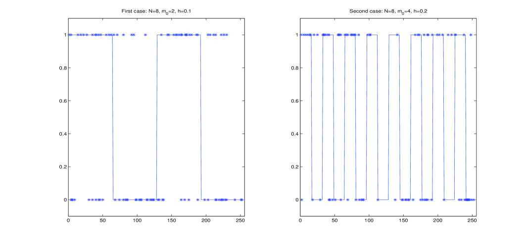
Figure 1: The plots of true functions and data for two cases.

Figure 1 plots true functions and observation data (with $n=100$) for two cases: first with $N=8,\ m_{0}=2,\ h=.1$, then $N=8,\ m_{0}=4,\ h=.2$. These pictures show how hard it is to decide intuitively what the true model is. Figure 2 plots LR criterion and RC criterion. Both criteria identify the true model in both cases.

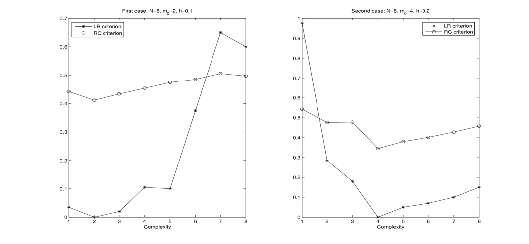
Figure 2: The plots of LR criterion and Rademacher complexity criterion.

Table 1 presents the proportions of correct identification over $100$ replications for each of $16$ cases with various sample sizes $n=50,\ 100,\ 200,\ 300$ and noise levels $h=.05,\ .1,\ .2,\ .3$ ($m_{0}=4$). It is shown that both criteria are model selection consistent as the proportions increases to 1 as $n$ and $h$ increase. The simulation suggests that the LR criterion has an improvement over the RC criterion for large sample sizes.

$n$	$h$	LR criterion	RC criterion	$n$	$h$	LR criterion	RC criterion
50	.05	.12	.13	200	.05	.23	.21
	.1	.35	.35		.1	.67	.66
	.2	.62	.64		.2	.99	.97
	.3	.95	.97		.3	1	1
100	.05	.15	.15	300	.05	.30	.28
	.1	.41	.41		.1	.78	.76
	.2	.89	.90		.2	1	.99
	.3	.98	.98		.3	1	1

Table 1: Proportions of correct identification of LR and RC criterion for various $n$ and $h$.

3 The LoRP for unsupervised learning

The LoRP developed so far is for supervised learning settings only. In supervised learnings, there are measurements called inputs which are used to predict outputs. Note that, in such settings, we have fixed the inputs $\boldsymbol{x}$ in the definition of the loss rank, and “resample” only the outputs $\boldsymbol{y}$. This seems to have some physical interpretation in supervised learnings and more importantly leads to a closed form of loss rank in many cases (Hutter and Tran, 2010). Such a way is not applicable to unsupervised learning settings where there is no outputs. For example, in graphical modelling or cluster analysis, the question of interest is to explore the associations between a set of input measurements. Fortunately, the basic reasoning of LoRP can be straightly extended to unsupervised learning. It is worth recalling the key observation of the LoRP: too flexible models will fit the actual data well and also fit fictitious/resampling data well (“fitting well” here means “having a small empirical loss”). Let $\boldsymbol{x}=(x_{1},...,x_{n})$ be the actual data set and $\text{\rm Loss}_{M}(x)$ be the empirical loss when fitting data $\boldsymbol{x}$ by a model $M$. Assume that the empirical loss has the property that the more flexible $M$, the smaller $\text{\rm Loss}_{M}(\boldsymbol{x})$. Let $\boldsymbol{x}^{\prime}$ be a resample from $\boldsymbol{x}$ using some resampling scheme (e.g., boostrapping). We can now define the loss rank of model $M$ as

$$\#\{\boldsymbol{x}^{\prime}:\text{\rm Loss}_{M}(\boldsymbol{x}^{\prime})\leq\text{\rm Loss}_{M}(\boldsymbol{x})\}.$$

This definition is easily understood intuitively but not very practical because the total number of resamples $\boldsymbol{x}^{\prime}$ is often huge or infinite. To make it more practical, we can proceed as follows. Let ${\cal B}$ be the set of $B$ resamples $\boldsymbol{x}^{\prime}$ from $\boldsymbol{x}$. The loss rank now can be defined as

$$\hat{\text{\rm LR}}_{B}(M|\boldsymbol{x})=\frac{\#\{\boldsymbol{x}^{\prime}\in{\cal B}:\text{\rm Loss}_{M}(\boldsymbol{x}^{\prime})\leq\text{\rm Loss}_{M}(\boldsymbol{x})\}}{B}.$$ (8)

Mathematically, let $\hat{\rm P}_{n}$ be the empirical probability measure of the resampling scheme (Efron and Tibshirani, 1993; van der Vaart and Wellner, 1996), we formally define the loss rank as

$$\text{\rm LR}(M|\boldsymbol{x})=\hat{\rm P}_{n}\{\boldsymbol{x}^{\prime}:\text{\rm Loss}_{M}(\boldsymbol{x}^{\prime})\leq\text{\rm Loss}_{M}(\boldsymbol{x})\}.$$ (9)

Clearly, the loss rank defined in (8) is an estimate of the one defined in (9). In the next section, we will study the unsupervised LoRP by means of simulation. The resampling scheme used is the popular bootstrap (Efron and Tibshirani, 1993).

4 Simulation studies for unsupervised LoRP

In this section, the unsupervised LoRP will be applied to selecting good models in graphical modelling and selecting number of clusters in cluster analysis.

4.1 LoRP for choosing number of clusters

Cluster analysis (Hastie et al., 2005, Ch.14) is an important problem in unsupervised learning. The goal is to group a collection of objects into clusters such that objects within each cluster are more closely related to each other than objects assigned to different clusters. In some applications, the number of clusters $K$ may be known in advance but in most cases $K$ is unknown and must be selected based on the data. Popular methods for model selection such as AIC, BIC or coss-validation are not applicable here (see, e.g., Hastie et al. (2005), Ch.14). Let $\boldsymbol{x}=(x_{1},...,x_{n})$ be $n$ objects and $d(x_{i},x_{j})$ be the distance (or dissimilarity measure) between $x_{i}$ and $x_{j}$. Suppose that the $n$ objects $\boldsymbol{x}$ have been clustered into $K$ clusters $C_{1},...,C_{K}$ using some clustering algorithm (e.g., the K-means algorithm). The natural loss is the within-cluster sum of dissimilarities

$$W_{K}(\boldsymbol{x})=\frac{1}{2}\sum_{k=1}^{K}\sum_{i,j\in C_{k}}d(x_{i},x_{j}).$$

When number of clusters $K$ increases, $W_{K}$ generally decreases. Let ${\cal B}$ be the set of $B$ bootstrap resamples $\boldsymbol{x}^{\prime}$ from the actual data $\boldsymbol{x}$, we define the loss rank of using $K$ clusters as in (8) by

$$\hat{\text{\rm LR}}_{B}(K|\boldsymbol{x})=\frac{\#\{\boldsymbol{x}^{\prime}\in{\cal B}:W_{K}(\boldsymbol{x}^{\prime})\leq W_{K}(\boldsymbol{x})\}}{B}.$$

The optimal $K$ selected by the LoRP will be $\hat{K}_{\text{\rm LR}}=\text{\rm arg}\min_{K}{\hat{\text{\rm LR}}}_{B}(K|\boldsymbol{x})$.

A popular method in the literature for selecting $K$ is the criterion proposed in Calinski and Harabasz (1974)

$$\text{CH}(K)=\frac{B_{K}/(K-1)}{W_{K}/(n-K)},$$

and the $K$ selected is the one maximizing this criterion. Note that the CH criterion is not defined for $K=1$. In the following simulation we compare the performance of the LoRP with that of the CH.

Simulation. We generate 2-dimensional datasets with various settings:

• 2 clusters, each with 50 observations, are generated from 2-dimensional normal distributions $N(\mu,\sigma I)$ with $\mu=(0,0),\ (0,5)$ and $\sigma=1,2,3$.

• 3 clusters, each with 50 observations, are generated from 2-dimensional normal distributions $N(\mu,\sigma I)$ with $\mu=(0,0),\ (0,5),\ (5,0)$ and $\sigma=1,2,3$.

• 4 clusters, each with 50 observations, are generated from 2-dimensional normal distributions $N(\mu,\sigma I)$ with $\mu=(0,0),\ (0,5),\ (5,0),\ (5,5)$ and $\sigma=1,2,3$.

We measure the performance in terms of percentage that the true number of clusters is correctly identified, over 100 replications for each setting. The simulation result is summarized in Table 2. It seems hard to compare the performance of the two methods. While the CH outperforms the LoRP for “easy” cases (small $\sigma$), the LoRP outperforms the CH for “hard” cases (large $\sigma$). However, our main interest is not the quality of the LoRP in this particular example, but to show that the unsupervised LoRP developed above as a general-purpose principle works for selecting number of clusters.

$\#$ clusters	$\sigma$	CH	LR
2	1	1	0.82
	2	1	0.74
	3	1	0.86
3	1	0.99	0.84
	2	0.7	0.45
	3	0	0.39
4	1	0.92	0.56
	2	0.04	0.38
	3	0	0.50

Table 2: Percentages of correct identification over 100 replications.

4.2 LoRP for graphical modelling

We study in this section the unsupervised LoRP for structural learning in graphical modelling, mainly focus on Markov networks with discrete-valued vertices (also called graphical log-linear modelling) (Whittaker, 1990; Edwards, 2000), but exactly the same idea would work for Bayesian networks as well.

Graphical modelling. The basic idea of graphical modelling is to use graphs to represent the independence structure among a set of variables. A graph is a pair $G=(V,E)$ where the vertex set $V$ consists of a finite set of random variables and the edge set $E$ represents the (conditional) independence relations between the r.v.’s in $V$. For every $u,v\in V$, if $u$ and $v$ are conditionally independent given all the other variables in $V$ then the edge $(u,v)$ is not included in $E$. In other words, a non-adjacent pair of vertices can be immediately interpreted as being conditionally independent given the rest. Graphical modelling provides an efficient way to represent and communicate the conditional independence relations between a set of r.v.’s. We restrict ourselves to undirected graphs (also called Markov networks) in this paper, but the same idea can be directly adapted for directed ones (or Bayesian networks).

Most of the literature on graphical modelling is concerned with selecting an appropriate model to explain the data. The most popular method is stepwise selection (Whittaker, 1990; Edwards, 2000) which starts at an initial base model and moves to next step by including or excluding a single edge until some termination criterion is fulfilled. Stepwise selection is search-efficient but its main drawback is that it may get stuck in a local optimum (Whittaker, 1990; Edwards, 2000). Furthermore, it is not easy to understand the statistical properties of the selected model.

Another criterion can be used for graphical model selection is the Bayesian information criterion (BIC) (Schwarz, 1978). BIC of model $G$ has the form

$$\text{BIC}(G)=-\log(\text{maximum likelihood under G})+\frac{1}{2}(\#\text{free parameters of $G$})\log n$$

It is well-known that BIC is asymptotically able to identify the true model (if it exists). One may use AIC (Akaike, 1973) as a selection criterion as well, but AIC tends to select overfitted models. AIC is optimal in terms of mean squared error loss (Shibita, 1984), however, this quantity is not well-defined in the graphical modelling context.

Loss rank criterion. Let $V$ be a set of $k$ discrete variables, and for each $v\in V$ let ${\cal I}_{v}$ be the set of its possible values/levels. The dataset of size $n$ is cross-classified by the levels of variables in $V$. Let ${\cal I}=\otimes_{v\in V}{\cal I}_{v}$. The dataset is often conveniently given in the form of a contingency table with cell counts $\boldsymbol{n}=\{n_{i}\}_{i\in{\cal I}}$ where $n_{i}$ is the observed number of observations cross-classified into cell $i$, $\sum n_{i}=n$. The sampling distribution of $\boldsymbol{n}$ is often assumed to be multinomial

$$p(\boldsymbol{n}|\boldsymbol{m})=\frac{n!}{\prod_{i\in{\cal I}}n_{i}!}\prod_{i\in{\cal I}}(\frac{m_{i}}{n})^{n_{i}},$$

where $\boldsymbol{m}=\{m_{i}\}_{i\in{\cal I}}$, $m_{i}$ are the expected numbers of observations falling into cells $i$ out of total $n$ observations, $\sum_{i}m_{i}=n$.

Let $\{\hat{m}_{i}(G,\boldsymbol{n})\}$ be the MLE of $m_{i}$ under model $G$. We define the empirical loss function resulting from fitting data $\boldsymbol{n}$ by model $G$ as the negative maximum log-likelihood (neglecting the constant terms depending only on $n$)

$$\text{\rm Loss}_{G}(\boldsymbol{n}):=-\sum_{i}\left[n_{i}\log(\hat{m}_{i}(G,\boldsymbol{n}))-\log(n_{i}!)\right].$$

This empirical loss is not a suitable measure for model selection, because the larger the model $G$ (w.r.t. inclusion), the smaller the loss. From (9), the loss rank of model $G$ is

$$\text{\rm LR}_{n}(G):=\hat{\rm P}_{n}\left(\text{\rm Loss}_{G}(\boldsymbol{n}^{\prime})\leq\text{\rm Loss}_{G}(\boldsymbol{n})\right)$$ (10)

where $\hat{\rm P}_{n}$ denotes the bootstrap empirical measure (Efron and Tibshirani, 1993) and $\boldsymbol{n}^{\prime}=\{n_{i}^{\prime}\}_{i\in{\cal I}}$ is a bootstrap resample from the actual data $\boldsymbol{n}$. The graph to be selected will be $\hat{G}_{\text{\rm LR}}=\text{\rm arg}\min\text{\rm LR}_{n}(G)$. We call this strategy the loss rank criterion for graphical model selection.

Similar to the classification case, it is straightforward to estimate the loss rank (10) by a simple Monte Carlo algorithm. In the following simulation, we estimate $\text{\rm LR}_{n}(G)$ by an average over $B=200$ bootstrap resamples $\boldsymbol{n}^{\prime}$ from $\boldsymbol{n}$. From our own experience, the result does not change much if a larger number of replications is used.

Note that definition (10) is somewhat similar to definition (5) of the loss rank for classification. However, the proof technique in Theorem 1 seems not to apply here because the derivations (6)-(7) in the proof are not valid anymore. Instead, in the following we will evaluate the suggested strategy by means of simulation. A theoretical justification is left for the future work.

In order to help the reader grasp better how the LR criterion works, we first present here a simple example where an exhaustive search over model space is possible. For the case of large number of vertices $k$, we will derive a genetic algorithm to overcome the difficulty in searching over huge model spaces.

A simple example. We consider a simple example where the number of vertices is $k=3$, and each variable takes on 3 values/levels. The number of graphs then is $2^{\binom{k}{2}}=8$. For a given sample size $n$, 100 datasets are generated from the “true” model with formula $12/23$, i.e., the first and third variable are conditionally independent given the second. We evaluate the performance in terms of proportion of correct identification over 100 replications. Table 3 shows the performance of LR in comparison to that of BIC.

$n$	200	500	1000	2000	5000
LR	.2	.7	.9	1	1
BIC	.05	.4	.7	.8	1

Table 3: Proportions of correct identification of LR and BIC for various $n$

The simulation result suggests that LR is superior to BIC. This result is similar to the simulation result in (Hutter and Tran, 2010, Table 1) in which it was also shown that the LoRP works better than BIC for model selection in linear regression.

Graphical model selection with LR criterion and a genetic algorithm. The main difficulty in graphical model selection is that the number of models is increasing more than exponentially as the number of vertices increases. Model selection can be seen as a problem of searching for the optimal solution, w.r.t. a certain selection criterion, over the model space. A natural choice is to adapt genetic algorithms (GA) (Holland, 1975; Mitchell, 1996) for searching over the model space. This idea has been already taken in (Poli and Roverato, 1998) who used AIC (Akaike, 1973) as the selection criterion and proposed a genetic algorithm for model search. Here, we adapt their genetic algorithm for model search and use the LR criterion as the selection criterion.

Genetic algorithms (Holland, 1975; Mitchell, 1996) are widely used to search for optimization solutions when the solution space is huge. The basic idea of GA is to mimic the evolutionary processes of creatures in which they attempt to find better solutions to the given problem by generating successive generations of individuals that are expected to be better suited to the environment than their ancestors.

Solutions are typically encoded by binary strings, called chromosomes. Chromosomes are associated with a fitness function and the problem is to find the fittest individual. The search space consists of all possible chromosomes, which is typically infeasible to access every individuals. A GA starts by generating an initial population and proceed by applying in turn three operators: selection, crossover and mutation. Selection operator randomly selects parents from the current population with probability being an increasing function of fitness to form a new population. At this stage, another operator called elitism may be used, in which a certain number of fittest individuals in the current population are directly inserted into the new population. Offsprings are obtained by applying the crossover to pairs of parents with a probability of $p_{c}$ - a pre-fixed number in $[0,1]$. The crossover typically consists in exchanging certain bits of two selected chromosomes. Finally, the new generation is obtained by applying with a probability of $p_{m}$ the mutation operator which changes one or more bits of a chromosome. The procedure is repeated until a termination criterion is satisfied. A widely-used termination criterion is that the fittest does not change for the last, say $T$, iterations. Some theoretical conditions to assure the convergence to the global optimal were introduced, however, applications do not always follow. Therefore, for the problem at hand, it is recommended to run the procedure several times before making the final decision of the selected fittest.

The specific application of GA to graphical model search consists in how to encode graphs as binary strings and in defining the operators selection, crossover and mutation.

Firstly, an undirected graph $G=(V,E)$ with $k$ vertices can be totally represented by a (strictly) upper triangular matrix ${\cal M}(G)=(m_{ij})_{j>i}$ in which $m_{ij}=1$ iff there is an edge between the $i$-th and $j$-th vertices. The matrix ${\cal M}(G)$ in turn can be identified with a binary string ${\cal B}(G)$ in which the entry $m_{ij}$ of ${\cal M}$ is stored at the corresponding position $(k-1)(i-1)+(j-1)-i(i-1)/2$ of ${\cal B}$. For example, the true model with formula 12/23 in the previous example can be encoded by the binary string $(1,0,1)$. The length of binary strings encoding graphs with $k$ vertices is $k(k-1)/2$.

The fitness function is inversely proportional to the loss rank: the fitter an individual, the smaller its loss rank. The fitness proportionate selection is not suitable in the present context, because some loss ranks may be very close or even equal to zero, which may cause premature convergence. Therefore the linear ranking selection (Mitchell, 1996) should be used. This selection operator starts by sorting the individuals in the decreasing (equivalently, increasing) order of fitness (loss rank). Then the probability for the $i$-th individual in the ranking to be selected is

$$p_{i}={\textstyle{1\over n}}\left(\beta-2(\beta-1){\textstyle{i-1\over n-1}}\right),\ \ \beta\in[1,2].$$

It seems that there is no clear suggestion on selection of $\beta$. In our simulation, $\beta$ is fixed to $1.5$. We also apply the elitism in which $5\%$ of the fittest individuals are kept for the next population before applying the selection operator.

We now follow Poli and Roverato (1998) to define the crossover operator. For a pair of parents models $G^{1}$ and $G^{2}$, a subset $A$ of $V$ is randomly selected and two offspring are formed by exchanging the induced subgraphs $G_{A}^{1},G_{A}^{2}$. The motivation of this operator is interpreted in Poli and Roverato (1998). The mutation operator consists in randomly selecting a bit in a binary string and change its value (0 to 1 and vice versa). The probability of doing crossover and mutation are fixed to $p_{c}=.9$ and $p_{m}=0.01$ respectively. These values are chosen based on our own experience and in reference to others

Some authors regard model selection as more than a machine learning or statistical issue, it is a philosophical one! Whether or not the true model exists is a controversial issue; another one is that whether or not one should select a single model and do subsequent inferences conditional on that selected one. It would be risky to select a single model, especially out of thousands as in the graphical modelling, and proceed as if it was the true one. Even if the true model exists, it is unrealistic to expect the GA to be always able to find. It is therefore more reasonable to restrict our expectation to finding a set of appropriate models instead of a single “best” one (which may turn out to be an inappropriate model!). The selected set then serves as the basic for a further context-specific consideration. The idea of selecting a set of models instead of a single model has also been discussed in Roverato and Paterlini (2004).

We now present the algorithm formally for searching for a set ${\cal H}$ of appropriate models. The maximum cardinality of such a set is pre-specified, say $K$. The basic idea is to repeat the GA procedure several times with different initial populations. We start with ${\cal H}=\emptyset$. After each iteration (of the GA procedure), a fittest individual is selected. This individual will be added to the optimal set ${\cal H}$ if it was not previously selected. The overall procedure stops when either the cardinality of ${\cal H}$ reaches $K$ or ${\cal H}$ does not change for the last, say $J$, iterations. The following is the GA-LR pseudo-code for our procedure. (the readers who are not familiar with GA are referred to Mitchell (1996) for the terminology).

• The GA-LR algorithm

  • ${\cal H}:=\emptyset$, $j:=0$, resampling $B$ resamples

  • While $|{\cal H}|\leq K$ and $j\leq J$ do

    • Generate an initial population $P$

    • Calculate the loss ranks for models in $P$ and select the fittest $G^{*}$

    • $t:=0$

      • While $t\leq T$ do

        • apply elitism and selection on $P$ to form new population $P_{1}$

        • apply crossover on $P_{1}$ to form $P_{2}$

        • apply mutation on $P_{2}$ to form $P_{3}$

        • $P:=P_{3}$

        • Calculate the loss ranks for $P$ and select the fittest $G^{\prime}$

        • If $G^{\prime}=G^{*}$ then $t:=t+1$ else $G^{*}:=G^{\prime};\ t:=0$

      • end while

    • If $G^{*}\in{\cal H}$ then $j:=j+1$ else ${\cal H}={\cal H}\cup\{G^{*}\};\ j:=0$

  • end while

A simulation study. We consider a moderate example with 6 vertices, each vertex takes on two values. The total number of graphs is $2^{\binom{6}{2}}=32768$. Datasets of size $n=10000$ are generated from the “true” model $123/456$. In our simulation, the parameters $T$ and $J$ are fixed to 5, the size of initial populations is fixed to 100. For a pre-specified maximum cardinality $K$, each run of the GA-LR algorithm produces a set ${\cal H}$ of optimal models in which $|{\cal H}|\leq K$. We are interested in whether or not the selected set ${\cal H}$ contains the true model. A small $K$ may be preferred because it eases the subsequent analysis, but important models are more likely to be missed. We evaluate the performance of selection criteria (LR and BIC) in terms of proportions in which the selected set ${\cal H}$ covers the true model. Table 4 shows those proportions over 10 replications for various $K$. From the simulation results, we draw the following conclusions: (i) The GA-BIC algorithm often terminates before the maximum $K$ is reached, i.e., the GA-BIC is more stable than the GA-LR; (ii) In contrast, the GA-BIC misses the true model more often than the GA-LR. An obvious drawback of the GA-LR is its computational time. In this simulation, each run of the GA-LR requires approximately 30 minutes which is about 50 times more than the running time of the GA-BIC.

$K$	10	20	50
GA-LR	.3	.6	.8
GA-BIC	.4	.5	.5

Table 4: Proportions of correct coverage for various $K$ over 10 replications

Remarks on computation aspects. The implementation is written in R, benefited from the R package igraph of Gabor Csardi. The simulation was carried out on a CPU Intel 2.66GHz. The software is freely available upon contacting the authors.

5 Conclusion

We have presented in this paper our continuous investigation of the LoRP, a general-purpose principle for model selection. The efficiency of the LoRP for model selection in classification was shown theoretically and experimentally. We also developed the LoRP for model selection in unsupervised learning settings and studied it by a means of simulation.

A fundamental question in model selection is that what kind of model one would like to select: the true model (i.e., the model generating the data) or a useful model in some sense (often, in terms of prediction) or a parsimonious model that fits the data not too bad. The LoRP attempts to deal with the latter which is, by common consent, the most appealing one in the machine learning community. Our objective in this paper is to draw the reader’s attention to a new methodology for model selection that seems to have a lot of potential, leading to a rich field.

References

- Akaike (1973) H. Akaike. Information theory and an extension of the maximum likelihood principle. In Proc. 2nd International Symposium on Information Theory, pages 267–281, Budapest, Hungary, 1973. Akademiai Kaidó.
- Allen (1974) D. Allen. The relationship between variable selection and data augmentation and a method for prediction. Technometrics, 16:125–127, 1974.
- Arlot (2008) S. Arlot. Model selection by resampling penalization. Electronic Journal Statist., 2008.
- Bartlett et al. (2002) P. Bartlett, S. Boucheron, and G. Lugosi. Model selection and error estimation. Machine Learning, 48:85–113, 2002.
- Bartlett et al. (2005) P. L. Bartlett, O. Bousquet, and S. Mendelson. Local rademacher complexities. Ann. Statist., 33(4):1497–1537, 2005.
- Calinski and Harabasz (1974) R. B. Calinski and J. Harabasz. A dendrite method for cluster analysis. Communications in Statistics, 3:1–27, 1974.
- Craven and Wahba (1979) P. Craven and G. Wahba. Smoothing noisy data with spline functions: estimating the correct degree of smoothing by the methods of generalized cross-validation. Numerische Mathematik, 31:377–403, 1979.
- Edwards (2000) David Edwards. Introduction to Graphical Modelling. Springer-Verlay New York, 2000. 2nd.
- Efron and Tibshirani (1993) B. Efron and R.J. Tibshirani. An Introduction to the Bootstrap. Chapman & Hall, 1993.
- Fan and Li (2001) J. Fan and R. Li. Variable selection via nonconcave penalized likelihood and its oracle properties. JASA, 96(456):1348–1360, 2001.
- Fromont (2007) M. Fromont. Model selection by bootstrap penalization for classification. Mach. Learn., 66:165–207, 2007.
- Gine and Zinn (1990) E. Gine and J. Zinn. Bootstrapping general empirical functions. Ann. Probab.., 18:851–869, 1990.
- Hastie et al. (2005) T. Hastie, R. Tibshirani, and J. H. Friedman. The Elements of Statistical Learning. Springer, 2005.
- Holland (1975) J. H. Holland. Adaption in Natural and Artificial Systems. University of Michigan Press, 1975.
- Hutter (2007) M. Hutter. The loss rank principle for model selection. In Proc. 20th Annual Conf. on Learning Theory (COLT’07), volume 4539 of LNAI, pages 589–603, San Diego, 2007. Springer, Berlin. URL http://arxiv.org/abs/math.ST/0702804.
- Hutter and Tran (2010) M. Hutter and M.-N. Tran. Model selection with the loss rank principle. Computational Statistics and Data Analysis, 54(5):1288–1306, 2010.
- Koltchinskii (2001) V. Koltchinskii. Rademacher penalties and structural risk minimization. IEEE Trans. Inform. Theory, 47:1902–1914, 2001.
- Koltchinskii (2006) V. Koltchinskii. Local rademacher complexities and oracle inequalities in risk minimization. Ann. Statist., 34(6):2593–2656, 2006.
- Lozano (2000) F. Lozano. Model selection using rademacher penalization. In Proc. 2nd ICSC Symp. Neural Computation NC2000. Berlin, Germany: ICSC Academic, 2000.
- Mallows (1973) C. L. Mallows. Some comments on . Technometrics, 15(4):661–675, 1973.
- Mitchell (1996) M. Mitchell. An Introduction to Genetic Algorithms. The MIT Press, 1996.
- Poli and Roverato (1998) I. Poli and A. Roverato. A genetic algorithm for graphical model selection. Journal of the Italian Statistical Society, 7(2):197–208, 1998.
- Rissanen (1978) J. J. Rissanen. Modeling by shortest data description. Automatica, 14(5):465–471, 1978.
- Roverato and Paterlini (2004) A. Roverato and S. Paterlini. Technological modelling for graphical models: an approach basedon genetic algorithms. Computational Statistics & Data Analysis, 47:323–337, 2004.
- Schwarz (1978) G. Schwarz. Estimating the dimension of a model. Annals of Statistics, 6(2):461–464, 1978.
- Shao (1996) J. Shao. Bootstrap model selection. Journal of the American Statistical Association, 91(434):655–665, 1996.
- Shibita (1984) R. Shibita. Approximate efficiency of a selection procedure for the number of regression variables. Biometrika, 71:43–49, 1984.
- Tibshirani (1996) R. Tibshirani. Regression shrinkage and selection via the lasso. J. R. Statist. Soc. B, 58(1):267–288, 1996.
- Tran (2009) M. N. Tran. Penalized maximum likelihood principle for choosing ridge parameter. Communications in Statistics - Simulation and Computation, 38:1610–1624, 2009.
- Tran (2010) M. N. Tran. The loss rank criterion for variable selection in linear regression analysis. Scandinavian Journal of Statistics, 2010. to appear.
- van der Vaart and Wellner (1996) A. W. van der Vaart and J. A. Wellner. Weak convergence and empirical processes. Springer, 1996.
- Vapnik and Chervonenkis (1971) V. N. Vapnik and A.Y. Chervonenkis. On the uniform convergence of relative frequencies of events to their probabilities. Theory Prob. its Application, 16:264–280, 1971.
- Whittaker (1990) J. Whittaker. Graphical Models in Applied Multivariate Statistics. Wiley, 1990.