Quasi-biennial oscillations in the solar tachocline caused by magnetic Rossby wave instabilities
Abstract
Quasi-biennial oscillations (QBO) are frequently observed in the solar activity indices. However, no clear physical mechanism for the observed variations has been suggested so far. Here we study the stability of magnetic Rossby waves in the solar tachocline using the shallow water magnetohydrodynamic approximation. Our analysis shows that the combination of typical differential rotation and a toroidal magnetic field with a strength G triggers the instability of the magnetic Rossby wave harmonic with a period of years. This harmonic is antisymmetric with respect to the equator and its period (and growth rate) depends on the differential rotation parameters and the magnetic field strength. The oscillations may cause a periodic magnetic flux emergence at the solar surface and consequently may lead to the observed QBO in the solar activity features. The period of QBO may change throughout the cycle, and from cycle to cycle, due to variations of the mean magnetic field and differential rotation in the tachocline.
1 Introduction
Apart from the well known 11-year cycle, solar activity shows quasi periodic variations on shorter time scales. Two different time scales have been frequently observed in many solar activity indicators: several months and a few years. The oscillations with period of several months (mostly with 150-160 days) are known as Rieger-type periodicities (Rieger et al., 1984; Lean & Brueckner, 1989; Carbonell & Ballester, 1990; Oliver et al., 1998; Krivova & Solanki, 2002; Kane, 2005; Knaack et al., 2005). The oscillations with period 2 years are known as Quasi-Biennial Oscillations (QBO) and they modulate almost all indices of solar activity (Sakurai, 1981; Gigolashvili et al., 1995; Knaack et al., 2005; Kane, 2005; Danilovic et al., 2005; Forgács-Dajka & Borkovits, 2007; Badalyan et al., 2008; Javaraiah et al., 2009; Laurenza et al., 2009; Vecchio & Carbone, 2009; Vecchio et al., 2010; Sýkora & Rybak, 2010).
The source(s) of these periodicities is still unclear. Several mechanisms have been suggested to drive the Rieger-type periodicities: interaction between and g-modes (Wolff, 1983), the timescale for storage and/or escape of magnetic fields in the solar convection zone (Ichimoto et al., 1985), “clock” modeled by an oblique rotator (Bai & Sturrock, 1991) and equatorially trapped Rossby-type waves in the photosphere (Lou, 2000). Recently, Zaqarashvili et al. (2010) (hereinafter Paper I) suggested that the Rieger-type periodicities can be caused by unstable , two-dimensional ( surface in spherical coordinates) magnetic Rossby waves in the solar tachocline. They show that a combination of the typical differential rotation parameters and the magnetic field strength G in the tachocline favor the strong growth of one particular harmonic with period of 150-160 days. The periodic modulation of the tachocline magnetic field due to the unstable harmonic triggers the periodic emergence of magnetic flux towards the surface, which leads to the observed periodicities in the solar activity. On the other hand, there is no clear mechanism for QBO reported in literature so far. Pataraya & Zaqarashvili (1995) supposed that the quasi 2-year impulse of shear waves can cause the 2-year periodicity of the differential rotation in the photosphere. However, this mechanism may work only near solar minima and cannot explain the long standing modulation of solar activity. Therefore, the question of the source for QBO is widely open.
In this letter, we show that the instability of magnetic Rossby waves in the tachocline could be the reason for QBO in solar activity. We consider a nonzero thickness of the tachocline and hence we use the shallow water magnetohydrodynamic (SWMHD) equations (Gilman, 2000). We show that a stronger magnetic field ( G) favors the growth of magnetic Rossby wave harmonic with period 2 years.
2 Shallow water MHD equations and unstable magnetic Rossby wave harmonics
In the following we use a spherical coordinate system rotating with the solar equator, where is the radial coordinate, is the co-latitude and is the longitude.
The solar differential rotation law in general is
| (1) |
where is the equatorial angular velocity, and are constant parameters determined by observations.
In the solar tachocline the magnetic field is predominantly toroidal, , and we take , where is in general a function of co-latitude. Then, the linear SWMHD equations (Gilman, 2000) can be rewritten in the rotating frame (with ) as follows:
| (2) |
| (3) |
| (4) |
| (5) |
| (6) |
where , , and are the velocity and magnetic field perturbations, is the tachocline thickness and is its perturbation, is the density, is the reduced gravity and is the distance from the solar center to the tachocline. Eqs. (5)-(6) are the solenoidal conditions of shallow water magnetic field and velocity respectively (Gilman, 2000).
Fourier analysis with and the transformation of variables in Eqs. (2)-(6) lead to the equations
| (7) |
| (8) |
where
are the Alfvén and surface gravity frequency respectively, is normalized by and
| (9) |
In the remaining we use a magnetic field
| (10) |
which changes sign at the equator (Gilman & Fox, 1997).
We expand and in infinite series of associated Legendre polynomials (Longuet-Higgins, 1968)
| (11) |
which satisfy the boundary conditions at (i.e. at the solar poles). Then, we substitute Eq. (11) into Eqs. (7)-(8) and, using a recurrence relation of Legendre polynomials, we obtain algebraic equations as infinite series. The dispersion relation for the infinite number of harmonics can be obtained when the infinite determinant of the system is set to zero. In order to solve the determinant, we truncate the series at , and the resulting polynomial in is solved numerically. This gives the frequencies of the first 70 harmonics. The harmonics with real frequency are stable, while those with complex frequency are unstable (see the general technique of Legendre polynomial expansion in Longuet-Higgins (1968); Watson (1981); Gilman & Fox (1997); Zaqarashvili et al. (2010) and references therein).
The typical values of equatorial angular velocity, radius and density in the tachocline are s-1, cm and g cm-3 respectively. We use a tachocline thickness cm. The ratio between angular and surface gravity frequencies is an important parameter in the shallow water theory. means strongly stable stratification (main part of tachocline), while considers weakly stable stratification (upper overshoot region). Here we consider the mean part of the tachocline and thus we take the limit .
The observed differential rotation parameters near the solar surface satisfy , which may tend to near the upper part of the tachocline (Schou et al., 1998). The solar radiative interior rotates uniformly, therefore the latitudinal differential rotation parameters drop to zero from the upper part of tachocline to its base. The radial dependence of latitudinal differential rotation through the tachocline is not clear, and may also vary throughout the solar cycle (Howe et al., 2000). Therefore, may take any value between 0.26 and 0.
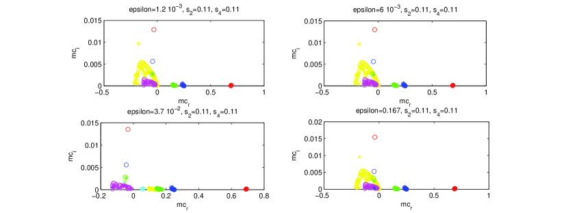
Figure 1 shows the real, , and imaginary, , frequencies of all unstable harmonics for different combinations of (i.e. reduced gravity) and magnetic field strength. The differential rotation parameters are fixed to . The plot shows that each combination of the magnetic field strength, differential rotation parameters and reduced gravity leads to the occurrence of a particular harmonic whose growth rate is much stronger than that of other harmonics. This is similar to what happens in the two-dimensional case (Zaqarashvili et al., 2010). An increase of magnetic field strength leads to the reduction of the frequency of the most unstable harmonic. The unstable harmonics are mostly symmetric (defined by asterisks) with respect to the equator for a magnetic field strength G, while they become mostly antisymmetric (defined by circles) for a strength G. A magnetic field strength between G yields unstable harmonics for both symmetries. This can be explained in terms of magnetic and differential rotation energies. Equipartition between the magnetic energy and the kinetic energy of differential rotation occurs at G for . When the magnetic field strength is smaller, then the differential rotation is the main energy source for instability and this obviously yields the symmetric harmonics as the differential rotation is symmetric around the equator. However, when the magnetic field is stronger, then the magnetic energy is the main source for the instability and the unstable harmonics are antisymmetric as the magnetic field is antisymmetric with respect to the equator.
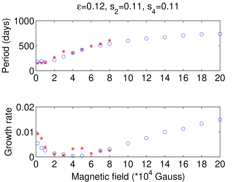
The importance of the equipartition value of the magnetic field strength is clearly seen on Figure 2. This figure displays the periods and growth rates (defined as ) vs magnetic field strength. The growth rates are higher for weaker ( G) and stronger ( G) magnetic fields. However, the growth rates are much lower when the magnetic field strength is inside the interval G. The weaker field ( G) favors Rieger-type periodicities (150-160 days), while the stronger field ( G) supports QBO. Increasing the magnetic field suppresses symmetric harmonics as it has been shown in Paper I.
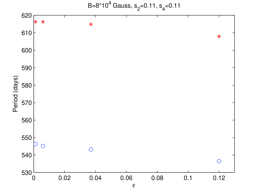
Figure 3 displays the period of the most unstable symmetric and antisymmetric harmonic vs the value of reduced gravity (i.e. on ) for a magnetic field strength of 8 G and the differential rotation parameters . It is seen that the oscillation period does not depend significantly on the reduced gravity.
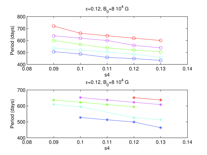
Figure 4 displays the dependence of the periods of the most unstable symmetric and antisymmetric harmonics on the differential rotation parameters for a magnetic field strength of 8 G and for (corresponding to a reduced gravity of cm s-2). The upper panel (circles) displays the antisymmetric harmonics and the lower panel (asterisks) displays the symmetric ones. The periods of unstable harmonics vs are plotted for different values of . The values of vary from 0.13 (blue color) to 0.09 (red color). We can observe that the period of this harmonic depends on the differential rotation parameters significantly and takes values between 400-700 days. The period becomes shorter for stronger differential rotation.
3 Discussion
Our results show that the differential rotation and the magnetic field with a strength of G may lead to large-scale oscillations of tachocline with periods of 2 years. The oscillation is due to the unstable mode of magnetic Rossby waves. The magnetic Rossby waves are magnetohydrodynamic counterparts to usual hydrodynamic Rossby waves (Zaqarashvili et al., 2007, 2009). The period and growth rate of the unstable harmonics depend on the magnetic field strength and the differential rotation parameters (Figures 1, 2 and 4). The unstable harmonics with periods of years are antisymmetric with respect to the solar equator.
The unstable magnetic Rossby waves in the tachocline can be the reason for QBO observed in almost all indices of the solar activity. Recent papers suggest that QBO are not persistent but may vary from cycle to cycle (Vecchio & Carbone, 2009) and throughout a cycle (Sýkora & Rybak, 2010). Our analyses also suggest this behaviour as the period of unstable harmonics depends on magnetic field strength and differential rotation parameters, which may vary in time depending on phase and strength of a particular cycle.
The antisymmetric behaviour of unstable harmonics with respect to the equator may explain the recent observational results of Badalyan et al. (2008), which show that QBO are well recognizable in the N-S asymmetry of solar activity indices.
Our analysis suggests the reduction of growth rates of unstable harmonics when the magnetic field strength is inside the interval G (see Figure 2). It is clearly seen that the relatively weak magnetic field G leads to the occurrence of Rieger-type periodicities (see the same results in the paper I), while the field of G favors QBO. The upper overshoot region of the tachocline probably contains relatively weaker magnetic field comparing to the lower stable layers. Therefore, we may speculate that the Rieger-type periodicities are formed in the overshoot layer (this was also suggested in the paper I), while QBO are formed in lower layers with strongly stable stratification. Therefore, the both periodicities may occur simultaneously.
The magnetic field of G is unstable due to the buoyancy instability, which makes difficult to keep it in the tachocline. On the other hand, the emergence of magnetic flux at observed latitudes requires sufficiently strong magnetic field () below the convection zone (Fan, 2004). Therefore, the storage of strong fields below the convection zone is still open question.
Significant simplifications in our approach is the linear stability analysis, which only describes the initial phase of instability. Intense numerical simulations are needed in the future to study the developed stage of magnetic Rossby wave instabilities.
4 Conclusions
We have shown that the unstable magnetic Rossby waves in the solar tachocline could be responsible for the observed intermediate periodicities in solar activity. The periods and growth rates of unstable harmonics depend on the differential rotation parameters and the magnetic field strength. The unstable harmonics are either symmetric or antisymmetric with respect to the equator. The latitudinal differential rotation is mainly responsible for the growth of symmetric harmonics, while, the antisymmetric toroidal magnetic field favors the growth of antisymmetric harmonics. A magnetic field with a strength G leads to oscillations with shorter period (150-170 days), while a stronger magnetic field G favors oscillations with longer periods (1-2.5 yrs). Hence, 2-year oscillations can be formed in the main part of the tachocline with stronger toroidal magnetic field and strongly stable stratification. The oscillations may trigger the periodic magnetic flux emergence at the solar surface and consequently QBO in solar activity.
Acknowledgements The authors acknowledge the financial support provided by MICINN and FEDER funds under grant AYA2006-07637. T. V. Z. acknowledges financial support from the Austrian Fond zur Förderung der wissenschaftlichen Forschung (under project P21197-N16), the Georgian National Science Foundation (under grant GNSF/ST09/4-310) and the Universitat de les Illes Balears.
References
- Badalyan et al. (2008) Badalyan, O. G., Obridko, V. N. and Sýkora, J., 2008, Sol. Phys., 247, 379
- Bai & Sturrock (1991) Bai T., & Sturrock P. 1991, Nature, 350, 141
- Carbonell & Ballester (1990) Carbonell, M., & Ballester, J.L. 1990, A&A, 238, 377
- Chowdhury et al. (2009) Chowdhury, P., Khan, M. & Ray, P.C., 2009, MNRAS, 392, 1159
- Danilovic et al. (2005) Danilovic, S., Vince, I., Vitas, N. & Jovanovic, P., 2005, Serb. Astron. J., 170, 79
- Fan (2004) Fan, Y. 2004, Living Reviews in Solar Physics, 1, 1
- Forgács-Dajka & Borkovits (2007) Forgács-Dajka, E. & Borkovits, T., 2007, MNRAS, 374, 282
- Gigolashvili et al. (1995) Gigolashvili, M. Sh., Japaridze, D. R., Pataraya, A. D. & Zaqarashvili, T.V., 1995, Sol. Phys., 156, 221
- Gilman & Fox (1997) Gilman, P. A. Fox, P. A. 1997, ApJ, 484, 439
- Gilman (2000) Gilman, P.A. 2000, ApJ, 484, 439
- Kane (2005) Kane, R.P., 2005, Sol. Phys., 227, 155
- Knaack et al. (2005) Knaack, R., Stenflo, J.O. & Berdyugina, S.V., 2005, A&A, 438, 1067
- Krivova & Solanki (2002) Krivova, N. A., & Solanki, S. 2002, A&A, 701
- Howe et al. (2000) Howe, R., Christensen-Dalsgaard, J., Hill, F., Komm, R. W., Larsen, R. M., Schou, J., Thompson, M. J. & Toomre, J., 2000, Science, 287, 2456
- Ichimoto et al. (1985) Ichimoto, K., Kubota, J., Suzuki, M., Tohmura, I., & Kurokawa, H. 1985, Nature, 316, 422
- Javaraiah et al. (2009) Javaraiah, J., Ulrich, R.K., Bertello, L. & Boyden, J.E., 2009, Sol. Phys., 257, 61
- Laurenza et al. (2009) Laurenza, M., Storini, M., Giangravé, S. & Moreno, G., 2009, J. Geophys. Res., 114, A01103
- Lean & Brueckner (1989) Lean, J., & Brueckner, G. E. 1989, ApJ, 337, 568
- Longuet-Higgins (1968) Longuet-Higgins, M. S. 1968, Proc. R. Soc. London. A, 262, 511
- Lou (2000) Lou, Y. Q. 2000, ApJ, 540, 1102
- Mursula & Vilppola (2004) Mursula, K. & Vilppola, J.H., 2004, Sol. Phys., 221, 337
- Oliver et al. (1998) Oliver, R., Ballester, J. L., & Baudin, F. 1998, Nature, 394, 552
- Pataraya & Zaqarashvili (1995) Pataraya, A. D. & Zaqarashvili, T.V., 1995, Sol. Phys., 157, 31
- Rieger et al. (1984) Rieger, E., Share, G. H., Forrest, D. J., Kanbach, G., Reppin, C., & Chupp, E. L. 1984, Nature, 312, 623
- Sakurai (1981) Sakurai, K., 1981, Sol. Phys., 74, 35
- Schou et al. (1998) Schou, J., Antia, H.M., Basu, S. et al., 1998, ApJ, 505, 390
- Sýkora & Rybak (2010) Sýkora, J. & Rybak, J., 2010, Sol. Phys., 261, 321
- Spiegel & Zahn (1992) Spiegel, E.A. & Zahn, J.-P., 1992, A&A, 265
- Vecchio & Carbone (2009) Vecchio, A. & Carbone, V., 2009, A&A, 502, 981
- Vecchio et al. (2010) Vecchio, A., Laurenza, M., Carbone, V. & Storini, M., 2010, ApJ, 709, L1
- Watson (1981) Watson, M. 1981, Geophys. Astrophys. Fluid dynamics, 16, 285
- Wolff (1983) Wolff, C. L. 1983, ApJ, 264, 667
- Zaqarashvili et al. (2007) Zaqarashvili, T. V., Oliver, R., Ballester, J. L. Shergelashvili, B. M. 2007, A&A, 470, 815
- Zaqarashvili et al. (2009) Zaqarashvili, T. V., Oliver, R. Ballester, J. L. 2009, ApJ, 691, L41
- Zaqarashvili et al. (2010) Zaqarashvili, T. V., Carbonell, M., Oliver, R. Ballester, J. L. 2010, ApJ, 709, 749