Conservation laws, integrability and transport in one-dimensional quantum systems

Abstract

In integrable one-dimensional quantum systems an infinite set of local conserved quantities exists which can prevent a current from decaying completely. For cases like the spin current in the $XXZ$ model at zero magnetic field or the charge current in the attractive Hubbard model at half filling, however, the current operator does not have overlap with any of the local conserved quantities. We show that in these situations transport at finite temperatures is dominated by a diffusive contribution with the Drude weight being either small or even zero. For the $XXZ$ model we discuss in detail the relation between our results, the phenomenological theory of spin diffusion, and measurements of the spin-lattice relaxation rate in spin chain compounds. Furthermore, we study the Haldane-Shastry model where the current operator is also orthogonal to the set of conserved quantities associated with integrability but becomes itself conserved in the thermodynamic limit.

I Introduction

In classical dynamics the KAM theorem quantitatively explains what level of perturbation can be exerted on an integrable system so that quasi-periodic motion survives.Arnol’d (1978) A classical system with Hamiltonian $H$ and phase space dimension $2N$ is integrable if $N$ constants of motion $Q_{k}$ exist (i.e., the Poisson bracket vanishes, $\{H,Q_{k}\}=0$) which are pairwise different, $\{Q_{k},Q_{l}\}=0$. Defining integrability for a quantum system is, however, much more complicated and no analogue of the KAM theorem is known. For any quantum system in the thermodynamic limit an infinite set of operators exist which commute with the Hamilton operator. This can be seen by considering, for example, the projection operators onto the eigenstates of the system, $[H,|n\rangle\langle n|]=0$ with $H|n\rangle=E_{n}|n\rangle$. In quantum systems described by tight-binding models with short-range interactions it is therefore important to distinguish between local conserved quantities $Q_{n}=\sum_{j}q_{n,j}$, where $q_{n,j}$ is a density operator acting on $n$ adjacent sites $j$, and nonlocal conserved quantities like the projection operators mentioned above. In a field theory, a conserved operator is local if it can be written as integral of a fully local operator. Most commonly, quantum systems are called integrable if an infinite set of local conserved quantities exists which are pairwise different. This definition includes, in particular, all Bethe ansatz integrable one-dimensional quantum systems. Here the local conserved quantities can be explicitly obtained by taking consecutive derivatives of the logarithm of the appropriate quantum transfer matrix with respect to the spectral parameter.Takahashi (1999)

In recent years, many studies have been devoted to the question if integrability can stop a system from thermalizingKinoshita et al. (2006); Hofferberth et al. (2007); Rigol et al. (2008) or a current from decaying completely.Castella et al. (1995); Zotos et al. (1997); Zotos (1999); Benz et al. (2005); Rosch and Andrei (2000); Alvarez and Gros (2002a, b); Fujimoto and Kawakami (2003); Jung and Rosch (2007a); Narozhny et al. (1998); Heidrich-Meisner et al. (2003); Jung et al. (2006); Klümper and Sakai (2002); Sirker et al. (2009) That conservation laws and the transport properties of the considered system are intimately connected is obvious in linear response theory (Kubo formula), which relates the optical conductivity to the retarded equilibrium current-current Green’s function. Specializing to a lattice model with nearest-neighbor hopping, the Kubo formula reads

$$\sigma(\omega)=\frac{i}{\omega}\left[\frac{\langle E_{\rm kin}\rangle}{L}+\langle\mathcal{J},\mathcal{J}\rangle_{\rm ret}(\omega)\right].$$ (1)

Here, $L$ is the system size, $T$ the temperature, $E_{\rm kin}$ the kinetic energy operator, $\mathcal{J}$ the spatial integral of the current density operator, and the brackets denote thermal average. The real part of the optical conductivity can be written as

$$\sigma^{\prime}(\omega)=2\pi D\delta(\omega)+\sigma_{reg}(\omega).$$ (2)

A nonzero Drude weight $D$ implies an infinite dc conductivity. Castella et al. [Castella et al., 1995] showed that it is possible to circumvent the direct calculation of the current-current correlation function in the Kubo formula and compute the finite temperature Drude weight using a generalization of Kohn’s formula.Kohn (1964) This formula relates the Drude weight to the curvature of the energy levels with respect to magnetic flux. The observation that integrable and nonintegrable models obey different level statistics,Berry and Tabor (1977); Bohigas et al. (1984); Poilblanc et al. (1993) as well as the calculation of the Drude weight from exact diagonalization for finite size systems,Zotos and Prelovšek (1996) led to the conjecture that anomalous transport, in the form of a finite $D(T>0)$, is a generic property of integrable models.Castella et al. (1995)

This conjecture is corroborated by the relation between the Drude weight and the long-time asymptotic behavior of the current-current correlation functionZotos et al. (1997)

$$D=\frac{1}{2LT}\lim_{t\to\infty}\langle\mathcal{J}(t)\mathcal{J}(0)\rangle\geq\frac{1}{2LT}\sum_{k}\frac{\langle\mathcal{J}Q_{k}\rangle^{2}}{\langle Q_{k}^{2}\rangle}\,.$$ (3)

In view of this relation, ballistic transport, $D\neq 0$, means that the current-current correlation function does not completely decay in time. The $Q_{k}$ operators in Eq. (3) form a set of commuting conserved quantities which are orthogonal in the sense that $\langle Q_{k}Q_{l}\rangle=\langle Q_{k}^{2}\rangle\delta_{kl}$. That conserved quantities provide a lower bound for the long-time asymptotic value of correlation functions is a general result due to MazurMazur (1969). In fact, it can be shown that the equality holds if the right-hand side of Eq. (3) includes all conserved quantities $Q_{k}$, local and non-local.Suzuki (1971)

The implications of Mazur’s inequality for transport in integrable quantum systems were pointed out by Zotos et al. [Zotos et al., 1997]. For integrable models where at least one conserved quantity $Q_{n}$ has nonzero overlap with the current operator, $\langle Q_{n}\mathcal{J}\rangle\neq 0$, Mazur’s inequality implies that the Drude weight is finite at finite temperatures. This happens, for instance, for charge transport in the Hubbard model away from half-filling and for spin transport in the $S=1/2$ $XXZ$ model at finite magnetic field. By contrast, for nonintegrable models, for which all local nontrivial conservation laws are expected to be broken, the right-hand side of Eq. (3) is expected to vanish so that $D(T>0)=0$. In these cases the delta function in Eq. (2) is generically presumed to be broadened into a Lorentzian Drude peak. The dc conductivity is finite and the system is said to exhibit diffusive transport.

However, in many cases of interest the known local conserved quantities associated with integrability are orthogonal to the current operator because of their symmetry properties. This happens, for instance in the $XXZ$ model at zero magnetic field $h$. In terms of spin-1/2 operators $\mathbf{S}_{l}$ the model reads

$$H=\sum_{l=1}^{N}[J(S_{l}^{x}S_{l+1}^{x}+S_{l}^{y}S_{l+1}^{y}+\Delta S_{l}^{z}S_{l+1}^{z})-hS_{l}^{z}].$$ (4)

Here $N$ is the number of sites, $\Delta$ parametrizes an exchange anisotropy, and $J$ is the exchange constant which we set equal to $1$ in the following. One can show that all local conserved quantities of the $XXZ$ model are even under the transformation $S_{j}^{z}\to-S_{j}^{z}$, $S_{j}^{\pm}\to S_{j}^{\mp}$, whereas the current operator is odd.Zotos et al. (1997) In these cases the integrability-transport connection has remained a conjecture. Nonetheless, several works have presented support for a finite Drude weight in models where the current operator has no overlap with the local conserved quantities, at least in some parameter regimes. The list of methods employed include exact diagonalization (ED),Narozhny et al. (1998); Heidrich-Meisner et al. (2003); Jung and Rosch (2007a); Rigol and Shastry (2008) Quantum Monte Carlo (QMC)Kirchner et al. (1999); Alvarez and Gros (2002b); Heidarian and Sorella (2007); Grossjohann and Brenig (2010) and Bethe ansatz (BA).Fujimoto and Kawakami (1998); Zotos (1999); Benz et al. (2005)

In particular for the $XXZ$ model, ED results for chains of lengths up to $L=18$ sitesHeidrich-Meisner et al. (2003) suggest that at high temperatures the Drude weight extrapolates to a finite value in the thermodynamic limit for values of exchange anisotropy in the critical regime, including the Heisenberg point. The Drude weight appears to vanish for large values of anisotropy in the gapped regime, but the minimum value of anisotropy for which it vanishes cannot be determined precisely. Although no conclusions can be drawn about the low temperature regime, the claim is that if the Drude weight is finite at high temperatures it must also be finite and presumably even larger at low temperatures. The weakness of this method is that it assumes that the finite size scaling of $D(T,L)$, which is not known analytically and is only obtained numerically for $L\leq 18$, can be extrapolated to the thermodynamic limit. This is not necessarily true for strongly interacting models where even at high temperatures there may be a large length scale above which the behavior of dynamical properties changes qualitatively.

In the QMC approach for the $XXZ$ model in Refs. [Alvarez and Gros, 2002a, b], the Drude weight was obtained by analytic continuation of the conductivity function $\sigma(q,i\omega_{n})$, which is a function of the Matsubara frequencies $\omega_{n}$, to real frequencies. This method uses a fitting function to try to extract a decay rate $\gamma$ which broadens the Drude peak if the Drude weight vanishes, but it clearly fails to find decay rates that are smaller than the separation between Matsubara frequencies, $\gamma\ll T$. In fact, the application of this method has even led to the conclusion that the Drude weight is finite for some gapless systems that are not integrable.Kirchner et al. (1999); Heidarian and Sorella (2007) This is hard to believe, considering that Eq. (3) requires the existence of nontrivial conservation laws which have a finite overlap with the current operator in the thermodynamic limit in order for the Drude weight to be finite. An attempt was made to explain the Drude weight for nonintegrable models described by a Luttinger liquid fixed point based on conformal field theoryFujimoto and Kawakami (2003), but this analysis neglects irrelevant interactions that lead to current decay and render the conductivity finite.Rosch and Andrei (2000)

Although the Drude weight for the $XXZ$ model has been calculated exactly by BA at $T=0$ using Kohn’s formula Shastry and Sutherland (1990), the calculation of $D(T>0)$ by BA is hindered by the need to resort to approximations in the treatment of the excited states. The BA calculation by ZotosZotos (1999) follows an ansatz proposed by Fujimoto and KawakamiFujimoto and Kawakami (1998) that employs the thermodynamic Bethe ansatz (TBA), which relies on the string hypothesis for bound states of magnons.Takahashi (1999) This approach predicts that the Drude weight is finite and decreases monotonically with $T$ for the $XXZ$ model in the critical regime at zero magnetic field, except at the Heisenberg point, where $D(T)$ vanishes for all finite temperatures. Benz et al. [Benz et al., 2005] criticized the TBA result and pointed out that it violates exact relations for $D(T)$ at high temperatures. These authors presented an alternative BA calculation of the Drude weight based on the spinon and anti-spinon particle basis and predicted a different temperature dependence than the TBA result. In particular, the Drude weight is found to be finite for the Heisenberg model at zero magnetic field. Actually, for values of anisotropy near the isotropic point this approach predicts that $D(T)$ increases with $T$ at low temperatures. Like the TBA result, the result based on spinons and anti-spinons violates exact relations at high temperatures. A consistent calculation of the Drude weight by applying the BA to the finite temperature Kohn formula is therefore still an unresolved issue.

Integer-spin Heisenberg lattice models are not integrable, but their low energy properties are often studied in the framework of the continuum O(3) nonlinear sigma model, which is integrable. Interestingly, BA calculations for the nonlinear sigma model predict a finite $D(T>0)$ that is exponentially small at temperatures below the energy gap.Fujimoto (1999); Konik (2003) In fact, it has been arguedKonik (2003) that the finite Drude weight is due to at least one nonlocal conserved quantity of the quantum model which is known explicitlyLüscher (1978) and has overlap with the current operator. This result is not consistent with the semiclassical results by Damle and SachdevDamle and Sachdev (1998, 2005), which predict diffusive behavior for gapped spin chains at low temperatures. No nonlocal conserved quantities that overlap with the current operator are known explicitly for the integrable $S=1/2$ $XXZ$ model. For finite chains such quantities can be constructed explicitly, however, in a numerical study of chains with $L\leq 18$ no definite conclusions could be made whether or not the overlap remains finite in the thermodynamic limit.Jung and Rosch (2007a)

The debate about the role of integrability in transport properties of integrable models is connected with the question of diffusion in $S=1/2$ spin chains. The term spin diffusion first appeared in the context of the phenomenological theory,Bloembergen (1949); de Gennes (1958); Steiner et al. (1976) where it refers to a characteristic form of long-time decay of the spin correlation function. In the phenomenological theory, the case where the total magnetization in the direction of quantization, $S^{z}=\sum_{j}S^{z}_{j}$, is conserved is considered. It is then said that spin diffusion occurs if the Fourier transform of the spin-spin correlation function $G(\mathbf{q},t)=\sum_{j}e^{-i\mathbf{q}\cdot(\mathbf{r}_{j}-\mathbf{r}_{0})}\langle S^{z}_{j}(t)S^{z}_{0}(0)\rangle$ for small wavevector $\mathbf{q}$ decays with time as $G(\mathbf{q},t)\sim e^{-D\mathbf{q}^{2}t}$, where $D$ is the diffusion constant. Provided that the behavior at small $q$ dominates, this implies that the Fourier transform decays as $G(\mathbf{r},t)\sim t^{-d/2}\exp(-|\mathbf{r}|^{2}/4Dt)$. This theory was formulated to explain results of inelastic neutron scattering experiments in three-dimensional ferromagnets at high temperatures. The assumptions of the theory are usually motivated by the picture that at high temperatures the spin modes are described by independent Gaussian fluctuations. The decay of the correlation function $G(\mathbf{r},t)$ can then be interpreted as a random walk of the magnetization through the lattice as in classical diffusion.

It is important to note that this definition of diffusion is not obviously related to that of diffusive transport given earlier, since the two definitions refer to two different correlation functions. In the phenomenological theory, transport is found to be diffusive because the local magnetization obeys the diffusion equation and the dc conductivity is therefore finite. However, more generally diffusion in the autocorrelation function for the density of the conserved quantity does not exclude the possibility of ballistic transport, understood as a nonzero long-time value for the current-current correlation function.

The applicability of the phenomenological theory of diffusion to spin chains described by the integrable $XXZ$ model is of course questionable. Even at high temperatures, the spin dynamics is likely to be constrained by the nontrivial conservation laws and the assumption of independent modes is not expected to hold. In the one case where the long-time behavior of the autocorrelation function can be calculated exactly, namely the XX model, which is equivalent to free spinless fermions, diffusion does not occur since $G(x=0,t)\sim t^{-1}$ for large $t$, as opposed to $t^{-1/2}$ expected for diffusion in one dimension. For decades, a great deal of effort has been made to compute the autocorrelation function for the $XXZ$ model with general values of anisotropy, particularly for the Heisenberg model.Carboni and Richards (1968); Böhm et al. (1994a, b); Fabricius et al. (1997); Fabricius and McCoy (1998); Starykh et al. (1997); Sirker (2006) While ED is always limited to small systems and short times (out to $t\sim 6$ in units of inverse exchange constant for $L=16$ sitesFabricius and McCoy (1998)), QMCStarykh et al. (1997) is plagued by the analytic continuation and cannot resolve singularities associated with the long-time behavior. Although the more recently developed density matrix renormalization group (DMRG) method applied to the transfer matrixSirker and Klümper (2005) works directly in the thermodynamic limit, it is also restricted to intermediate times and has not detected a diffusive contribution at low temperatures.Sirker (2006) Nonetheless, these works have concluded in favor of the existence of diffusion for the Heisenberg model at high temperatures.

Although diffusion was originally proposed to describe spin dynamics at high temperatures, the paradigm has been used to interpret nuclear magnetic resonance (NMR) experiments that measure the spin-lattice relaxation rate $1/T_{1}$ of spin chains at low temperatures.Boucher et al. (1976); Takigawa et al. (1996a); Thurber et al. (2001); Kikuchi et al. (2001) Strictly speaking, linear response theory expresses $1/T_{1}$ in terms of the Fourier transform of the transverse spin-spin correlation function $\langle S^{+}_{j}(t)S^{-}_{j^{\prime}}(t)\rangle$. The small magnetic field applied in NMR experiments breaks the rotational spin invariance of Heisenberg chains from SU(2) down to U(1) and the total $S^{\pm}$ are not conserved. However, if the experiments are in the regime of temperatures small compared to the exchange constant, but large compared to the nuclear or electronic Larmor frequencies then the transverse correlation function can be traded for the longitudinal one calculated for the electronic Larmor frequency. We will discuss this point in more detail in Section II.7. Up to $q$-dependent form factors that stem from the spatial dependence of the hyperfine couplings, $1/T_{1}$ is then proportional to the dynamical autocorrelation $G(\boldsymbol{r}=0,\omega)$, with $\omega\propto h$ equal to the Larmor frequency of an electron in a magnetic field $h$. If diffusion is present, with $G(\boldsymbol{r}=0,t)\sim t^{-d/2}$ given as in the phenomenological theory, $1/T_{1}$ behaves as $1/T_{1}\propto G(\boldsymbol{r}=0,\omega)\sim\omega^{d/2-1}$ in $d$ dimensions. In particular, in the one-dimensional case $1/T_{1}$ diverges at low frequencies as $1/T_{1}\sim 1/\sqrt{\omega}\sim 1/\sqrt{h}$. This type of behavior has been observed for gapped $S=1$ spin chainsTakigawa et al. (1996b) and gapless spin chains with large half-integer $S$.Boucher et al. (1976) More surprisingly, spin diffusion has also been observed in $S=1/2$ chain compounds by NMRThurber et al. (2001); Kikuchi et al. (2001) and by muon spin resonance.Pratt et al. (2006) It is important to note that in the NMR experiment of Ref. [Thurber et al., 2001], the $q$-dependence of the form factor suppresses the contribution from $q\sim\pi$ modes in the autocorrelation function, so that the $1/T_{1}$ signal is completely dominated by $q\sim 0$ modes.

The observation of spin diffusion in $S=1/2$ Heisenberg chains is puzzling from the point of view of the integrability-transport conjecture. Since the experimental diffusion constant was found to be fairly large,Thurber et al. (2001) it becomes important to determine whether the diffusion constant is mainly determined by integrability-breaking interactions present in the real system or by umklapp processes already contained in the integrable Heisenberg model.

Recently, we have shown using a field theory approach that the long-time behavior of the autocorrelation function and the transport properties are directly related and can be obtained from the same retarded Green’s function at low temperatures.Sirker et al. (2009) The analytical results were supported by DMRG calculations for the time-dependent current-current correlation function as well as by a comparison with the NMR experiment on Sr₂CuO₃.Thurber et al. (2001) We also argued that ballistic transport can be reconciled with diffusion in the autocorrelation function because ballistic channels of propagation can coexist with diffusive ones. This can be made precise with the help of the memory matrix approach,Rosch and Andrei (2000) which allows one to incorporate known conservation laws in the low energy effective theory. However, ballistic and diffusive channels compete for spectral weight of the spin-spin correlation function. Our field theoretical results for the $XXZ$ chain at $h=0$ – valid at finite temperatures small compared to the exchange energy – are in very good agreement with the diffusive response measured experimentallyThurber et al. (2001) and with time-dependent DMRG results if we assume that the Drude weight vanishes completely. Although a small Drude weight at finite temperatures cannot be excluded, a combination of the numerical data with the memory matrix approach implies that it has to be smaller than the values obtained in the BA calculation by Klümper et al. [Benz et al., 2005] and by QMC calculationsAlvarez and Gros (2002a, b). The results in Ref. [Sirker et al., 2009] were further supported by a recent QMC study.Grossjohann and Brenig (2010) In the latter work the problems arising from analytical continuation of numerical data were circumvented by comparing with the field theory resultSirker et al. (2009) transformed to imaginary times.

The purpose of this paper is to provide details of the calculations for the $XXZ$ chain in Ref. [Sirker et al., 2009]. Furthermore, we present an extension of these methods to charge transport in the attractive Hubbard model as well as a discussion of the transport properties of the Haldane-Shastry chain. Our paper is organized as follows: In Sec. II we study the spin current in the spin-$1/2$ Heisenberg chain. We discuss the relation between the current-current and the spin-spin correlation function at low temperatures, explain in detail how our results relate to previous BA and QMC calculations, and discuss consequences for electron spin resonance and the finite-temperature broadening of the dynamic spin structure factor. In Sec. III, we discuss spin transport in the Haldane-Shastry model and point out that the current operator is a nonlocal conserved quantity in the thermodynamic limit. In Sec. IV we show that many of the results we obtained for the spin current in the Heisenberg model also directly apply to the charge current in the attractive Hubbard model. Finally, we give a summary and some conclusions in Sec. V.

II The spin current in the spin-$1/2$ $XXZ$ model

The $XXZ$ model (4) is exactly solvable by Bethe ansatz (BA) Giamarchi (2004) and for $h=0$ the excitation spectrum is gapless for $|\Delta|\leq 1$ and gapped for $|\Delta|>1$.

The spin-current density operator is defined from the continuity equation for the density of the globally conserved spin component

$$\partial_{t}S^{z}_{l}=-i[S^{z}_{l},H]=-(j_{l}-j_{l-1}),$$ (5)

which for the $XXZ$ model yields

$$j_{l}=-\frac{iJ}{2}(S_{l}^{+}S_{l+1}^{-}-S_{l+1}^{+}S_{l}^{-}).$$ (6)

For $h\neq 0$, the summed current operator $\mathcal{J}=\sum_{l}j_{l}$ has a finite overlap with the local conserved quantities of the $XXZ$ model. The simplest nontrivial conserved quantity is

$$\mathcal{J}_{E}=J^{2}\sum_{l}\left[S^{y}_{l-1}S^{z}_{l}S^{x}_{l+1}-S^{x}_{l-1}S^{z}_{l}S^{y}_{l+1}+\Delta(S^{x}_{l-1}S^{y}_{l}S^{z}_{l+1}-S^{z}_{l-1}S^{y}_{l}S^{x}_{l+1})+\Delta(S^{z}_{l-1}S^{x}_{l}S^{y}_{l+1}-S^{y}_{l-1}S^{x}_{l}S^{z}_{l+1})\right].$$ (7)

Here $\mathcal{J}_{E}$ is the energy current operator as obtained from the continuity equation for the Hamiltonian density for $h=0$ Zotos et al. (1997); Klümper and Sakai (2002). It can be verified that $\mathcal{J}_{E}$ is conserved in the strong sense that $[\mathcal{J}_{E},H]=0$. The thermal conductivity therefore only has a Drude part which can be calculated exactly by BA.Klümper and Sakai (2002) According to Mazur’s inequality, Eq. (3), the overlap of $\mathcal{J}$ with $\mathcal{J}_{E}$ provides a lower bound for the Drude weight of the spin conductivity

$$D\geq D_{\rm Mazur}\equiv\frac{1}{2LT}\frac{\langle\mathcal{J}\mathcal{J}_{E}\rangle^{2}}{\langle\mathcal{J}_{E}^{2}\rangle}.$$ (8)

The advantage of this formula is that – contrary to Eq. (1) – it does not require the calculation of dynamical correlation functions and is thus much more accessible by standard techniques. The evaluation of (8) becomes particularly simple in the limit $T\to\infty$ leading toZotos et al. (1997)

$$D_{\rm Mazur}=\frac{J}{T}\frac{4\Delta^{2}m^{2}(1/4-m^{2})}{1+8\Delta^{2}(1/4+m^{2})}\qquad(T\gg J),$$ (9)

where $m=\langle S_{l}^{z}\rangle$ is the magnetization. At low temperatures, on the other hand, standard bosonization techniques can be applied. Furthermore, BA can be used to evaluate (8) for all temperatures as will be shown in Sec. II.1.

All other local conserved quantities can be obtained either recursively by applying the so-called boost operatorZotos et al. (1997) or by taking higher order derivatives of the quantum transfer matrix of the $XXZ$ Hamiltonian with respect to the spectral parameter. The local operators obtained this way act on more and more adjacent sites but they are all even under particle-hole transformations. As a result, the Mazur bound for the Drude weight, Eq. (3), vanishes for $h=0$.

II.1 Low energy effective model and the Mazur bound

Bosonization of the $XXZ$ model, Eq. (4), in the gapless regime at zero field leads to the effective Hamiltonian Giamarchi (2004); Eggert and Affleck (1992); Lukyanov (1998)

$$H = H_{0}+H_{\rm u}+H_{\rm bc},$$

$$H_{0} = \frac{v}{2}\int dx\left[\Pi^{2}+(\partial_{x}\phi)^{2}\right],$$

$$H_{\rm u} = \lambda\int dx\cos(\sqrt{8\pi K}\phi),$$ (10)

$$H_{\rm bc} = -2\pi v\lambda_{+}\int dx(\partial_{x}\phi_{R})^{2}(\partial_{x}\phi_{L})^{2}$$

$$- 2\pi v\lambda_{-}\int dx\left[(\partial_{x}\phi_{R})^{4}+(\partial_{x}\phi_{L})^{4}\right]\;.$$

Here, $H_{0}$ is the standard Luttinger model and $H_{\rm u}$ and $H_{\rm bc}$ are the leading irrelevant perturbations due to Umklapp scattering and band curvature, respectively. The bosonic field $\phi=\phi_{R}+\phi_{L}$ and its conjugate momentum $\Pi$ obey the canonical commutation relation $[\phi(x),\Pi(x^{\prime})]=\text{i}\delta(x-x^{\prime})$. The long-wavelength ($q\sim 0$) fluctuation part of the spin density is related to the bosonic field by $S^{z}_{j}\sim\sqrt{K/2\pi}\partial_{x}\phi$. The spin velocity and the Luttinger parameter $K$ are known exactly from Bethe ansatz

$$v=\frac{\pi\sqrt{1-\Delta^{2}}}{2\arccos\Delta}\quad,\quad K=\frac{\pi}{\pi-\arccos\Delta}\;.$$ (11)

In this notation, $K=2$ at the free fermion point ($\Delta=0$) and $K=1$ at the isotropic point ($\Delta=1$). The amplitudes $\lambda$, $\lambda_{+}$, and $\lambda_{-}$ are also known exactlyLukyanov (1998)

$$\lambda = \frac{K\Gamma(K)\sin(\pi/K)}{\pi\Gamma(2-K)}\left[\frac{\Gamma\left(1+\frac{1}{2K-2}\right)}{2\sqrt{\pi}\Gamma\left(1+\frac{K}{2K-2}\right)}\right]^{2K-2},$$

$$\lambda_{+} = \frac{1}{2\pi}\tan\frac{\pi K}{2K-2},$$ (12)

$$\lambda_{-} = \frac{1}{12\pi K}\frac{\Gamma\left(\frac{3K}{2K-2}\right)\Gamma^{3}\left(\frac{1}{2K-2}\right)}{\Gamma\left(\frac{3}{2K-2}\right)\Gamma^{3}\left(\frac{K}{2K-2}\right)}.$$

In the gapless phase, the Mazur bound can be calculated in the low-temperature regime using the field theory representations of $\mathcal{J}$ and $\mathcal{J}_{E}$. In the continuum limit, the continuity equation becomes

$$\partial_{t}S^{z}(x)+\partial_{x}j(x)=0.$$

Using the bosonized form for the spin density, we obtain for the effective model (II.1)

$$\mathcal{J} = -\sqrt{\frac{K}{2\pi}}\int dx\,\partial_{t}\phi$$

$$= -v\sqrt{\frac{K}{2\pi}}\int dx\left[\Pi-\frac{\pi}{2}(\lambda_{+}+2\lambda_{-})\Pi^{3}\right.$$

$$- \left.\frac{\pi}{2}(-\lambda_{+}+6\lambda_{-})\Pi\,(\partial_{x}\phi)^{2}\right].$$

In the following we neglect the corrections to the current operator due to band curvature terms and calculate the Mazur bound $D_{\rm Mazur}$ for the Luttinger model $H_{0}$ using the current operator

$$\mathcal{J}\approx-v\sqrt{\frac{K}{2\pi}}\int dx\,\Pi$$ (14)

and the energy current operator

$$\mathcal{J}_{E}\approx-v^{2}\int dx\,\Pi\,\partial_{x}\phi.$$ (15)

At zero field, the overlap vanishes because $\mathcal{J}$ and $\mathcal{J}_{E}$ have opposite signatures under the particle-hole transformation $\phi\to-\phi,\Pi\to-\Pi$. A small magnetic field term in Eq. (4), on the other hand, can be absorbed by shifting the bosonic field (here we set $\mu_{B}=1$)

$$\phi\to\phi+\frac{h}{v}\sqrt{\frac{K}{2\pi}}x.$$ (16)

In this case, the conserved quantity becomes Rosch and Andrei (2000)

$$\tilde{\mathcal{J}}_{E}=-v^{2}\int dx\,\Pi\,\partial_{x}\phi-hv\sqrt{\frac{K}{2\pi}}\int dx\,\Pi=\mathcal{J}_{E}+h\mathcal{J}.$$ (17)

We calculate the equal time correlations within the Luttinger model and find

$$D_{\rm Mazur}=\frac{1}{2TL}\frac{\langle\mathcal{J}\tilde{\mathcal{J}}_{E}\rangle^{2}}{\langle\tilde{\mathcal{J}}_{E}^{2}\rangle}=\frac{vK/4\pi}{1+\frac{2\pi^{2}}{3K}\left(\frac{T}{h}\right)^{2}}\qquad(T,h\ll J).$$ (18)

We note that in the limit $T/h\to 0$ the Mazur bound obtained from the overlap with $\tilde{\mathcal{J}_{E}}$ saturates the exact zero temperature Drude weight $D(T=0)=vK/4\pi$ Shastry and Sutherland (1990).

One can also use the Bethe ansatz to calculate the Mazur bound in Eq. (8) exactly. To do so we computed the equal time correlations using a numerical solution of the nonlinear integral equations obtained within the Bethe ansatz formalism of Refs. [Sakai and Klümper, 2005; Bortz and Göhmann, 2005]. In Fig. 1, the numerical Bethe ansatz solution for small values of magnetization $m$ is compared to the field theory formula (18).

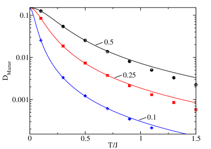
Figure 1: Mazur bound $D_{\rm Mazur}$ as defined in (8) for $\Delta=\cos(\pi/4)$ and magnetic fields $h$ as indicated on the plot. The symbols correspond to the exact calculation using the Bethe ansatz, the lines represent the field theoretical formula (18).

Remarkably, the free boson result in Eq. (18) fits well the behavior of the exact Mazur bound out to temperatures of order $J$.

II.2 Retarded spin-spin correlation function

We will now proceed with the field theory calculations in the following way. We first assume that the Drude weight is not affected by unknown nonlocal conserved quantities. In this case we are left with the following picture based on the Mazur bound and including all conserved quantities related to integrability: For finite magnetic field the Drude weight is a continuous function of temperature. At zero field, however, the Drude weight is only finite at $T=0$ but drops abruptly to zero for arbitrarily small temperatures. Within the effective field theory such a possible broadening of the delta-function peak at finite temperatures has to be related to inelastic scattering between the bosons which can relax the momentum. Such a process is described by the Umklapp term in Eq. (II.1) which we have ignored so far. We will now include this term as well as the band curvature terms in a lowest order perturbative calculation. We want to stress that such an approach does not know about conservation laws which could protect a part of the current from decaying. The parameter-free result derived here is expected to be correct if the Drude weight is indeed zero and allows to check the validity of the assumption by comparing with experimental and numerical results. Importantly, we can also systematically study how this result is modified if such conservation laws do exist after all. This case will be considered in section II.3.

We are interested in the retarded spin-spin correlation function $\chi_{\rm ret}(q,\omega)$, which can be obtained from the Matsubara correlation function

$$\chi(q,i\omega_{n})=-\frac{1}{N}\sum_{l,l^{\prime}}^{N}e^{-iq(l-l^{\prime})}\int_{0}^{1/T}d\tau\,e^{i\omega_{n}\tau}\langle S_{l}^{z}(\tau)S_{l^{\prime}}^{z}(0)\rangle$$ (19)

by the analytic continuation $i\omega_{n}\to\omega+i0^{+}$. We will show that in the low-temperature limit this correlation function determines both the decay of the current-current correlation function as well as the spin-lattice relaxation rate $1/T_{1}$. In the low-energy limit, we follow Ref. [Oshikawa and Affleck, 1997] and relate the long-wavelength part of the retarded spin-spin correlation function to the boson propagator

$$\frac{\chi_{\rm ret}(q,\omega)}{Kq^{2}/2\pi}=\langle\phi\phi\rangle^{\rm ret}(q,\omega)=\frac{v}{\omega^{2}-v^{2}q^{2}-\Pi^{\rm ret}(q,\omega)}.$$ (20)

We calculate the self-energy $\Pi^{\rm ret}(q,\omega)=\Pi_{\rm u}^{\rm ret}(q,\omega)+\Pi_{\rm bc}^{\rm ret}(q,\omega)$ by perturbation theory to second order in $H_{\rm u}$ and first order in $H_{\rm bc}$. We first focus on the half-filling case ($h=0$); the finite field case is discussed at the end of this sub-section.

The contribution from Umklapp scattering reads

$$\Pi_{\rm u}^{\rm ret}(q,\omega)=4\pi Kv\lambda^{2}\left[F^{\rm ret}(q,\omega)-F^{\rm ret}(0,0)\right],$$ (21)

where Schulz (1986)

$$F^{\rm ret}(q,\omega) = -\frac{v}{T^{2}}\left(\frac{\pi T}{v}\right)^{4K}\sin(2\pi K)$$

$$\times I\left(\frac{\omega+vq}{2T}\right)I\left(\frac{\omega-vq}{2T}\right),$$

with

$$I(z)=\int_{0}^{\infty}\frac{\text{e}^{izu}\,du}{\sinh^{2K}(\pi u)}=\frac{2^{2K-1}}{\pi}B\left(K-\frac{iz}{2\pi},1-2K\right),$$ (23)

where $B(x,y)=\Gamma(x)\Gamma(y)/\Gamma(x+y)$ is the beta function. For $K>1/2$, we need a cutoff in the integral $I(z)$ in Eq. (23). However, the imaginary part of $I(z)$ does not depend on the cutoff scheme used Schulz (1986). The expansion of Eq. (23) for $|\omega\pm vq|\ll T$ yields both a real and an imaginary part for $\Pi_{\rm u}^{\rm ret}(q,\omega)$. The calculation of $\Pi_{\rm bc}^{\rm ret}(q,\omega)$ is also standard. In contrast to $\Pi_{\rm u}^{\rm ret}(q,\omega)$, the result for $\Pi_{\rm bc}^{\rm ret}(q,\omega)$ is purely real, as band curvature terms do not contribute to the decay rate. The end result is

$$\Pi^{\rm ret}(q,\omega)\approx-2i\gamma\omega-b\omega^{2}+cv^{2}q^{2}.$$ (24)

In the anisotropic case, $-1<\Delta<1$, the parameters are given by

$$2\gamma = Y_{1}T^{4K-3}$$

$$b = \underbrace{(Y_{2}-Y_{3})T^{4K-4}}_{b_{2}}+\underbrace{Y_{4}T^{2}}_{b_{1}}$$ (25)

$$c = \underbrace{-(Y_{2}+Y_{3})T^{4K-4}}_{c_{2}}\underbrace{-Y_{4}T^{2}}_{c_{1}}.$$

Here $b_{1}$ and $c_{1}$ ($b_{2}$ and $c_{2}$) are the parts stemming from the band curvature (umklapp) terms, respectively. In Eq. (II.2) we have used the following functions

$$Y_{1} = \Lambda\frac{B(K,1-2K)}{\sqrt{\pi}2^{2K+1}}\cot(\pi K),$$

$$Y_{2} = \Lambda\frac{B(K,1-2K)}{\pi^{5/2}2^{2K+4}}(\pi^{2}-2\Psi^{\prime}(K)),$$

$$Y_{3} = \Lambda\frac{1}{\pi 2^{4K+4}}\cot^{2}(\pi K)\Gamma(1/2-K)\Gamma(K),$$ (26)

$$Y_{4} = \frac{\pi^{2}}{6v^{2}}(\lambda_{+}+6\lambda_{-}),$$

$$\Lambda = 4\pi K\lambda^{2}\sin(2\pi K)\left(\frac{2\pi}{v}\right)^{4K-2}\Gamma(1/2-K)\Gamma(K),$$

with $\Psi(x)$ being the Digamma function.

At the isotropic point, $\Delta=1$, Umklapp scattering becomes marginal and can be taken into account by replacing the Luttinger parameter by a running coupling constant, $K\to 1+g(T)/2$. In this case we find

$$2\gamma = \pi g^{2}T,$$

$$b = \frac{g^{2}}{4}-\frac{g^{3}}{32}\left(3-\frac{8\pi^{2}}{3}\right)+\frac{\sqrt{3}}{\pi}T^{2},$$ (27)

$$c = \frac{g^{2}}{4}-\frac{3g^{3}}{32}-\frac{\sqrt{3}}{\pi}T^{2}.\;$$

Following Lukyanov Lukyanov (1998), the running coupling constant $g(T)$ is determined by the equation

$$\frac{1}{g}+\frac{\ln g}{2}=\ln\left[\sqrt{\frac{\pi}{2}}\frac{\text{e}^{1/4+\tilde{\gamma}}}{T}\right],$$ (28)

where $\tilde{\gamma}$ is the Euler constant. We remark that a similar calculation was attempted in Ref. [Fujimoto and Kawakami, 2003], but there the imaginary part of the self-energy was neglected.

This calculation can be extended to finite magnetic field. Shifting the field $\phi$ as in Eq. (16), the Umklapp term in Eq. (10) becomes $H_{\rm u}=\lambda\int dx\cos[\sqrt{8\pi K}\phi+(2Kh/v)x]$. As long as $h\ll T$, it is reasonable to keep this oscillating term in the effective Hamiltonian. However, in a renormalization group treatment, after we lower our momentum cut-off below $h$, it should be dropped. Our formula for the self-energy, in Eq. (21) is thus modified to

$$\Pi_{\rm u}^{\rm ret}(q,\omega) = 2\pi Kv\lambda^{2}\left[F^{\rm ret}(q+2Kh/v,\omega)\right.$$

$$+ F^{\rm ret}(q-2Kh/v,\omega)$$

$$- \left.F^{\rm ret}(2Kh/v,0)-F^{\rm ret}(-2Kh/v,0)\right],$$

where $F^{\rm ret}(q,\omega)$ is given by Eqs. (II.2) and (23) as before. As a consequence, the relaxation rate for $h/T\ll 1$ will now be given by $\gamma\sim T^{4K-3}[1+\mathcal{O}[(h/T)^{2}]+\cdots]$ (up to logarithmic corrections in the isotropic case). In the next section we show that the retarded current-current correlation function can be obtained at low energies using the calculated self-energy. We will also discuss what the shortcomings of the self-energy approach are and show that these shortcomings can be addressed by taking conservation laws into account explicitly.

II.3 Decay of the current-current correlation function

The time-dependent current-current correlation function can be written as

$$C(t) \equiv \frac{1}{L}\langle\mathcal{J}(t)\mathcal{J}\rangle$$

$$= -2\int_{-\infty}^{\infty}\frac{d\omega}{2\pi}\,\frac{e^{-i\omega t}}{1-e^{-\omega/T}}\,{\rm Im}\langle\mathcal{J};\mathcal{J}\rangle_{\rm ret}(\omega),$$

where $\langle\mathcal{J};\mathcal{J}\rangle_{\rm ret}(\omega)$ is the retarded current-current correlation function. The latter appears in the Kubo formula for the optical conductivity (1) with $\langle E_{\rm kin}\rangle/L=Kv/2\pi$ and the current operator given by $\mathcal{J}=-\sqrt{K/2\pi}\partial_{t}\phi$. One can easily show that

$$\langle\partial_{t}\phi\partial_{t}\phi\rangle^{ret}(q,\omega)=-v+\omega^{2}\langle\phi\phi\rangle^{ret}(q,\omega)$$ (31)

leading to

$$\langle\mathcal{J};\mathcal{J}\rangle^{ret}(q,\omega)=-\frac{Kv}{2\pi}+\frac{K}{2\pi}\omega^{2}\langle\phi\phi\rangle^{ret}(q,\omega)\;.$$ (32)

The Kubo formula (1) can therefore also be written as

$$\sigma(q,\omega)=\frac{K}{2\pi}\text{i}\omega\langle\phi\phi\rangle^{ret}(q,\omega)$$ (33)

allowing us to use the results for the boson-boson Green’s function from the previous section. At zero temperature the irrelevant operators in (II.1) can be ignored and the Drude weight of the $XXZ$ model can be obtained using the free boson propagator

$$\langle\phi\phi\rangle^{ret}(q,\omega)=\frac{v}{\omega^{2}-v^{2}q^{2}}\;.$$ (34)

implying

$$D(T=0)\delta(\omega) \equiv \frac{1}{2\pi}\lim_{\omega\to 0}\lim_{q\to 0}\sigma^{\prime}(q,\omega)$$

$$= \frac{Kv}{4\pi^{2}}\textrm{Re}\left[\frac{i}{\omega+\text{i}\epsilon}\right]=\frac{Kv}{4\pi}\delta(\omega)$$

in agreement with Bethe ansatz.Shastry and Sutherland (1990)

If we now turn to finite temperatures we can use the result from the self-energy approach in Eqs. (20, 24) and relation (33), leading to the optical conductivity

$$\sigma(q,\omega)=\frac{Kv}{2\pi}\frac{\text{i}\omega}{(1+b)\omega^{2}-(1+c)v^{2}q^{2}+2\text{i}\gamma\omega}$$ (36)

with the real part being given by

$$\sigma^{\prime}(q,\omega)=\frac{Kv\omega}{2\pi}\frac{2\gamma\omega}{[(1+b)\omega^{2}-(1+c)v^{2}q^{2}]^{2}+(2\gamma\omega)^{2}}.$$ (37)

For $q=0$ we find, in particular, a Lorentzian

$$\sigma^{\prime}(\omega)=\frac{vK}{2\pi}\frac{2\gamma}{[(1+b)\omega]^{2}+(2\gamma)^{2}}.$$ (38)

As expected, the self-energy approach predicts zero Drude weight whenever $\gamma(T)$ is nonzero. This result is inconsistent with Mazur’s inequality if there exist conservation laws which protect the Drude weight. We know that this is the case for any arbitrarily small magnetic field $h$, while our calculations in sub-section IIB gave a non-zero $\gamma$ at non-zero field. Whether or not such a conservation law exists also for $h=0$ is an open question. We will try to tackle this problem by first studying how the self-energy result is modified by a conservation law, followed by a comparison with numerical and experimental results.

It is possible to accommodate the existence of nontrivial conservation laws by resorting to the memory matrix formalism of Ref. [Rosch and Andrei, 2000]. This approach starts from the Kubo formula for a conductivity matrix $\hat{\sigma}$ which includes not only the current operator $\mathcal{J}\equiv\mathcal{J}_{1}$, but also “slow modes” $\mathcal{J}_{n}$ ($n\geq 2$) which have a finite overlap with $\mathcal{J}$. The idea is that if $\langle\mathcal{J}_{n}(t)\mathcal{J}_{n}(0)\rangle$ is a slowly decaying function of time, the projection of $\mathcal{J}$ into $\mathcal{J}_{n}$ governs the long-time behavior of the current-current correlation function and consequently dominates the low-frequency transport. The overlap between $\mathcal{J}$ and the slow modes is captured by the off-diagonal elements of the conductivity matrix. In practice, only a small number of conserved quantities is included in the set of slow modes, but the approach can be systematically improved since adding more conserved quantities increases the lower bound for the conductivity Jung and Rosch (2007b). It is convenient to invert the Kubo formula for the conductivity matrix using the projection operator method Jung and Rosch (2007b). We introduce the scalar product between two operators $A$ and $B$ in the Liouville space

$$(A|B)=\frac{T}{L}\int_{0}^{1/T}d\tau\,\langle A^{\dagger}e^{H\tau}Be^{-H\tau}\rangle.$$ (39)

Here, $\mathcal{L}$ is the Liouville superoperator defined by $\mathcal{L}\mathcal{J}_{n}=[H,\mathcal{J}_{n}]$. For simplicity, we assumed that all the slow modes have the same signature under time-reversal symmetry. The conductivity matrix can be written as

$$\sigma_{nm}(\omega)=i\left(\mathcal{J}_{n}|(\omega-\mathcal{L})^{-1}|\mathcal{J}_{m}\right).$$ (40)

The conductivity in Eq. (1) is the $\sigma_{11}$ component of $\hat{\sigma}$. The susceptibility matrix $\hat{\chi}$ is defined as

$$\chi_{nm}=T^{-1}(\mathcal{J}_{n}|\mathcal{J}_{m}).$$ (41)

We denote by

$$\mathcal{P}=1-T^{-1}\sum_{nm}\chi^{-1}_{nm}|\mathcal{J}_{n})(\mathcal{J}_{m}|$$ (42)

the projector out of the subspace of slow modes. Using identities for the projection operator, Eq. (40) can be brought into the form Rosch and Andrei (2000)

$$\sigma_{nm}(\omega)=i\{[\omega-\hat{M}\hat{\chi}^{-1}]^{-1}\hat{\chi}\}_{nm},$$ (43)

where $\hat{M}$ is the memory matrix given by

$$M_{nm}=T^{-1}(\mathcal{J}_{n}|\mathcal{L}\mathcal{P}\frac{1}{\omega-\mathcal{P}\mathcal{L}\mathcal{P}}\mathcal{P}\mathcal{L}|\mathcal{J}_{m}).$$ (44)

It can be shown that if there is an exact conservation law (local or nonlocal) involving one of the slow modes, the memory matrix has a vanishing eigenvalue, which then implies a finite Drude weight.

In the following we apply the memory matrix formalism to calculate the conductivity for the low-energy effective model (II.1) at $h=0$, allowing for the existence of a single conserved quantity $Q$, $[Q,H]=0$. The conductivity matrix is then two-dimensional. We choose $\mathcal{J}_{1}=\mathcal{J}$ and $\mathcal{J}_{2}=Q_{\perp}\equiv Q-\mathcal{J}(\mathcal{J}|Q)(\mathcal{J}|\mathcal{J})^{-1}$ so that $\hat{\chi}$ is diagonal. At low temperatures $T\ll J$, we can use the current operator in Eq. (II.1); to first order in $\lambda_{\pm}$, we obtain

$$\chi_{11}\approx\frac{\langle\mathcal{J}^{2}\rangle}{LT}\approx\frac{vK}{2\pi}(1-b_{1}),$$ (45)

where $b_{1}$ is defined in Eq. (II.2) and we have used the fact that due to the vanishing of the superfluid density we have $\langle E_{\rm kin}\rangle/L\approx\langle\mathcal{J}^{2}\rangle/LT$. Likewise, $\chi_{22}=(\langle Q^{2}\rangle-\langle QJ\rangle^{2}/\langle J^{2}\rangle)/(LT)$ can be calculated within the low energy effective model once a conserved quantity $Q$ has been identified. The remaining approximation is in the calculation of the memory matrix to second order in Umklapp. This is analogous to the calculation of the self-energy $\Pi^{\rm ret}_{\rm u}$ in Eq. (21). Using the conservation law, we can write

$$\hat{M}\approx M_{11}(\omega)\left(\begin{array}[]{cc}1&-r\\ -r&r^{2}\end{array}\right),$$ (46)

where $r=\langle Q\mathcal{J}\rangle/\langle\mathcal{J}^{2}\rangle$ and

$$M_{11}(\omega)\approx\frac{vK}{2\pi}\frac{\Pi_{\rm u}(\omega)}{\omega}\approx\frac{vK}{2\pi}(-b_{2}\omega-2i\gamma),$$ (47)

with $b_{2}$ as given in Eq. (II.2). Thus, from equation (43), we find

$$\sigma(\omega)=\chi_{11}\left[\frac{y}{1+y}\frac{i}{\omega}+\frac{1}{1+y}\frac{i}{\omega-(1+y)\chi_{11}^{-1}M_{11}(\omega)}\right],$$ (48)

where

$$y=\frac{r^{2}\chi_{11}}{\chi_{22}}=\frac{\langle\mathcal{J}Q\rangle^{2}}{\langle\mathcal{J}^{2}\rangle\langle Q^{2}\rangle-\langle\mathcal{J}Q\rangle^{2}}.$$ (49)

For finite magnetic field, a conserved quantity is given by $Q=\mathcal{J}_{E}+h\mathcal{J}$ (see Eq. (17)) and thus $y\sim(h/T)^{2}$ in this case. Equating Eq. (36) for $q=0$ and (48), we find that the memory matrix approach is equivalent to adopting the self-energy

$$\Pi(\omega)\approx\frac{\omega\chi_{11}^{-1}M_{11}(\omega)-b_{1}\omega^{2}}{1-y\chi_{11}^{-1}M_{11}(\omega)/\omega}=\frac{-b\omega^{2}-2i\gamma\omega}{1-y\chi_{11}^{-1}M_{11}(\omega)/\omega}.$$ (50)

As expected, the memory matrix result reduces to the self-energy result for $y\to 0$. The difference between the self-energy and the memory matrix result is of higher order in the Umklapp interaction. Therefore, the conservation law is not manifested in the lowest-order calculation of the self-energy. Although Eq. (50) is not correct beyond $O(\lambda^{2},\lambda_{\pm})$, it suggests that the memory matrix approach corresponds to a partial resummation of an infinite family of Feynman diagrams which changes the behavior of $\Pi(\omega)$ in the limit $\omega\to 0$ from $\Pi\to-2i\gamma\omega$ to $\Pi\to-y^{-1}\omega^{2}$.

It follows from Eq. (1) and Eq. (48) that

$${\rm Im}\langle\mathcal{J};\mathcal{J}\rangle_{\rm ret}(\omega) = -\omega{\rm Re}\,\sigma(\omega)$$

$$= -\omega\frac{vK}{2\pi}\left[\frac{\pi y(1-b_{1})}{1+y}\,\delta(\omega)\right.$$

$$+ \left.\frac{2\gamma}{(1+b_{1}+b_{2}^{\prime})^{2}\omega^{2}+(2\gamma^{\prime})^{2}}\right],$$

where $b_{2}^{\prime}=(1+y)b_{2}$ and $\gamma^{\prime}=(1+y)\gamma$. The first term on the right hand side of Eq. (II.3) can be associated with the ballistic channel and the second one with the diffusive channel. The calculation is valid also in the finite field case if $h/T\ll 1$ with $y\sim(h/T)^{2}$ as already discussed below Eq. (48). This means that we obtain a correction of the relaxation rate in the memory matrix formalism which is exactly of the same order as obtained previously from the self-energy approach in this limit (see Eq. (II.2)). However, now we see that the weight is transferred accordingly from the diffusive into a ballistic channel, a fact which is missed in the self-energy approach.

Substituting Eq. (II.3) into Eq. (II.3) we can now evaluate the integral. From the second term in (II.3) we obtain an integrand which has poles at frequencies $\omega=\pm 2\text{i}\gamma^{\prime}/(1+b_{1}+b_{2}^{\prime})$ and $\omega=2\pi\text{i}Tn$ with $n\in\mathbb{Z}$. Since $2\gamma^{\prime}\ll 2\pi T$ the contributions of the latter poles can be ignored at times $t\gg(2\pi T)^{-1}$ leading to

$$C(t)=\frac{Kv}{2\pi(1+y)}\left[yT(1-b_{1})-\frac{2\text{i}\gamma^{\prime\prime}}{1+b_{1}+b_{2}^{\prime}}\frac{\text{e}^{-2\gamma^{\prime\prime}t}}{1-\text{e}^{2\text{i}\gamma^{\prime\prime}/T}}\right]$$ (52)

with $\gamma^{\prime\prime}=\gamma^{\prime}/(1+b_{1}+b_{2}^{\prime})$. We can further expand the denominator in powers of $\gamma^{\prime\prime}/T\ll 1$. The first order contribution is real and given by

$$C(t)\sim\frac{vKT}{2\pi(1+y)}\left[y(1-b_{1})+\frac{e^{-2\gamma^{\prime}t}}{1+b_{1}+b_{2}^{\prime}}\right].$$ (53)

The imaginary part of the correlation function is obtained in second order in the expansion and is thus suppressed by an additional power of $\gamma^{\prime}/T$. From Eq. (53) we see that in the limit $t\to\infty$ the current-current correlation function approaches the value

$$\lim_{t\to\infty}C(t)=\frac{vKTy(1-b_{1})}{2\pi(1+y)}\approx\frac{\langle\mathcal{J}^{2}\rangle y}{L(1+y)}=\frac{\langle\mathcal{J}Q\rangle^{2}}{L\langle Q^{2}\rangle},$$ (54)

consistent with the Mazur bound for the Drude weight. For intermediate times $(2\pi T)^{-1}\ll t\ll 1/\gamma^{\prime}$, we obtain the linear decay

$$C(t)\approx\frac{vKT}{2\pi(1+b)}(1-2\gamma t),$$ (55)

independent of $y$ if $b_{1},b_{2}^{\prime}\ll 1$. Therefore a small Drude weight cannot be detected in this intermediate time range.

II.4 Comparison with Bethe ansatz and numerical data for the current-current correlation function

In the previous section we have derived a result for the optical conductivity, Eq. (II.3), and for the real part of the current-current correlation function, Eq. (53), at low temperatures by a memory-matrix formalism. In this approach we have explicitly taken into account the possibility of a nonlocal conservation law - leading to a nonzero Drude weight at finite temperatures. By comparing our results with the Bethe ansatz calculationsZotos (1999); Benz et al. (2005) and numerical calculations of $C(t)$ we will show that a diffusive channel for transport does indeed exist. Furthermore, we will try to obtain a rough bound for how large $y$ and therefore the Drude weight $D(T)$ can possibly be.

A finite Drude weight at finite temperatures has been obtained in two independent Bethe ansatz calculationsZotos (1999); Benz et al. (2005), however, the obtained temperature dependence is rather different. In both works the finite temperature Kohn formulaCastella et al. (1995), which relates the Drude weight and the curvature of energy levels with respect to a twist in the boundary conditions, is used. While Zotos [Zotos, 1999] uses a TBA approach based on magnons and their bound states, Klümper et al. [Benz et al., 2005] use an approach based on a spinon and anti-spinon particle basis. Both approaches have been shown to violate exact relations at high temperatures and are therefore not exact solutions of the problem. The reason is that within the Bethe ansatz both approaches use assumptions which have been shown to work in the thermodynamic limit for the partition function. This, however, does not seem to be the case for the curvature of energy levels relevant for the Drude weight. Nevertheless, this does not exclude that these results become asymptotically exact at low temperatures and arguments for such a scenario have been given in Ref. [Benz et al., 2005].

To investigate this possibility we start by comparing in Fig. 2 the Bethe ansatz results from Ref. [Benz et al., 2005] at low temperatures with the Drude weight

$$D(T)=\frac{Kv}{4\pi(1+b)}$$ (56)

obtained by setting $\gamma=0$ in Eq. (36). We see from Eq. (53) that this corresponds to the case $y\to\infty$, i.e., in this case there is only a ballistic channel.

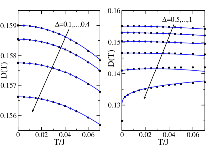
Figure 2: The Bethe ansatz results from Ref. [Benz et al., 2005] (dots) compared to the field theory formula (56) (lines) obtained by setting $\gamma=0$ by hand in Eq. (36). The $\Delta$ values are indicated on the plot.

Doing so we obtain excellent agreement. From this we draw two conclusions: First, this BA calculation predicts that even at finite temperatures the transport is purely ballistic. Second, the temperature dependent parameter $b$ which we obtained from field theory in first order in band curvature and second order in Umklapp scattering is consistent with this BA approach. We note that the case $\Delta=1/2$ ($K=3/2$) is particularly interesting because here the contributions $b_{1}$ from band curvature and $b_{2}$ from Umklapp scattering in Eq. (II.2) both yield a $T^{2}$ contribution with diverging prefactors. These divergencies cancel leading to a Drude weight

$$D(T)=\frac{9\sqrt{3}}{32\pi}\frac{1}{1+\tilde{b}T^{2}}$$ (57)

with $\tilde{b}=[142+24\tilde{\gamma}+48\ln 2+60\ln 3-24\ln T-21\zeta(3)]/243$ where $\tilde{\gamma}$ is the Euler constant and $\zeta$ the Riemann zeta function. As is also the case for other thermodynamic quantitiesSirker and Bortz (2006) we see that the coinciding scaling dimensions of the terms stemming from Umklapp scattering and band curvature lead to a term $\sim T^{2}\ln T$ at this special point. For $\Delta<1/2$ ($K>3/2$) band curvature gives the dominant temperature dependence while Umklapp scattering dominates for $\Delta>1/2$ ($K<3/2$). For $K>5/4$ ($\Delta\gtrsim 0.81$) a $T^{8K-8}$ term, which arises in 4th order perturbation theory in Umklapp scattering and which is not included in our calculations, becomes more important than the $T^{2}$ term from band curvature. Therefore the agreement for $\Delta=0.9$ in Fig. 2 is not quite as good as for the other values. For $\Delta=1$, Umklapp scattering becomes marginal leading to a logarithmic temperature dependence of the Drude weight (56) with $b$ as given in (II.2).

To see whether or not such a large Drude weight as predicted by Klümper et al. is possible and to discuss the second BA approach by Zotos we now turn to a numerical calculation of $C(t)$. A dynamical correlation function at finite temperatures can be obtained by using a density matrix renormalization group algorithm applied to transfer matrices (TMRG).Sirker and Klümper (2005); Sirker (2006); Sirker et al. (2009) This algorithm uses a Trotter-Suzuki decomposition to map the 1D quantum model onto a 2D classical model. For the classical model a so-called quantum transfer matrix can be defined which evolves along the spatial direction and allows one to perform the thermodynamic limit exactly. In order to calculate dynamical quantities, a complex quantum transfer matrix is considered with one part representing the thermal density matrix and the other part the unitary time evolution operator. By extending the transfer matrix one can either lower the temperature (imaginary time) or increase the real time interval for the correlation function. The calculation of the current-current correlation function is particularly complicated because it involves the summation of all the local time-dependent correlations

$$\frac{1}{L}\langle\mathcal{J}(t)\mathcal{J}(0)\rangle=\sum_{l}\langle j_{l}(t)j_{0}(0)\rangle$$ (58)

with the current density $j_{l}$ as given in Eq. (6). In Fig. 3 the local correlations $\langle j_{l}(t)j_{0}(0)\rangle$ are exemplarily shown for the case $\Delta=0.6$ and $T/J=0.2$.

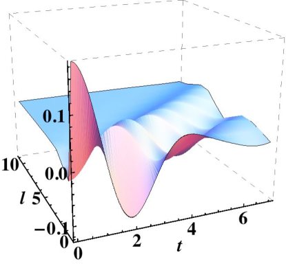
Figure 3: $\langle j_{l}(t)j_{0}(0)\rangle$ for $\Delta=0.6$ at $T/J=0.2$.

In order to obtain converged results, the two-point correlations for distances up to $l\sim 30$ have to be summed up. This is not possible using exact diagonalization which is restricted to considerably smaller system sizes. A good check is obtained by considering the free fermion case $\Delta=0$. Here $\langle j_{l}(t)j_{0}(0)\rangle$ can be calculated exactly and is non-trivial, however, $\mathcal{J}=\sum_{l}j_{l}$ commutes with the Hamiltonian leading to (58) being a constant.

We now discuss the same parameter set $\Delta=0.6$ and $T/J=0.2$ as used above in more detail. In Fig. 4 the real and imaginary parts of $C(T)/2JT$, obtained in a TMRG calculation with a $1000$ states per block kept, are shown. Because the imaginary part is very small, an extrapolation in the Trotter parameter was necessary restricting the calculations to smaller times than for the real part.

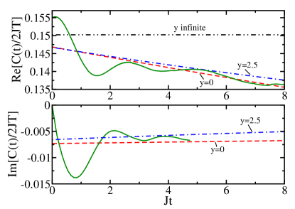
Figure 4: Real and imaginary parts of the current correlation function for $\Delta=0.6$ and $T/J=0.2$. The dashed, dot-dashed and dotted lines correspond to formula (52) with $y$ values as indicated on the plot.

In the limit $t\to\infty$, the real part would directly yield the Drude weight (possibly zero). As already discussed, the BA result by Klümper et al. corresponds to purely ballistic transport, $y\to\infty$. From Fig. 4 we see that this is not consistent with the numerical data. The BA calculation by Zotos, on the other hand, predicts a Drude weight $\sim 0.105$ which requires $y\sim 2.5$. While formula (52) with $y=0$ seems to fit the numerical results best, we would need to be able to simulate slightly longer times (a factor of $1.5-2$ should be sufficient) to clearly distinguish between $y=0$ and $y=2.5$. Most importantly, however, the numerical data clearly demonstrate that the decay rate $\gamma$ is nonzero.

In addition to the zero field case, we have also calculated $C(t)$ at relatively large magnetic fields and various temperatures. As shown in Fig. 5 we find that in such cases $C(t)$ appears to converge to a finite value within fairly short times.

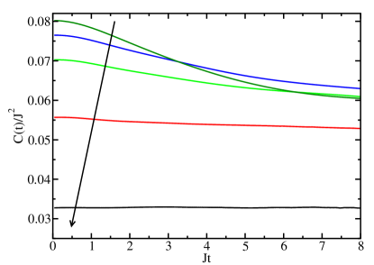
Figure 5: $C(t)$ for $\Delta=0.4$ and a magnetization $\langle m\rangle=0.3$ at temperatures $T/J=20,1,0.\bar{6},0.4,0.2$ (in arrow direction). At low temperatures the asymptotic value seems to be reached almost instantaneously. At high temperatures the data seem to be consistent with a simple exponential decay to a finite value without oscillations. Using an exponential fit and extrapolating to infinite temperature we find $C(T\to\infty,t\to\infty)\approx 0.058$. On the other hand, the Mazur bound, Eq. (9), yields $2TD_{\mbox{Mazur}}=0.013$.

Furthermore, we find (see Fig. 6) that at large $\Delta$ and large magnetic fields the Mazur bound (9) almost completely exhausts the Drude weight at high temperatures. This is consistent with the findings in Ref. [Zotos et al., 1997] which were based on exact diagonalization.

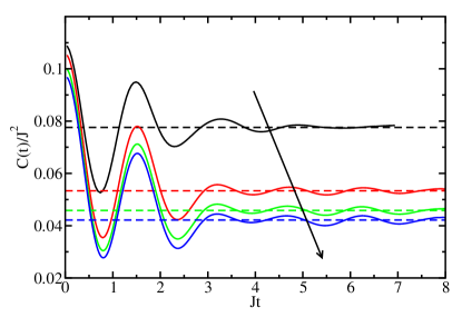
Figure 6: $C(t)$ for $\Delta=4.0$ and a magnetization $\langle m\rangle=0.25$ with $T/J=1,5,10,20$ (in arrow direction). In addition, linear fits of the data in the regime $Jt\geq 4$ are shown (dashed lines). Extrapolating these values we find $C(T\to\infty,t\to\infty)\approx 0.0385$. In this case the Mazur bound, Eq. (9), yields $2TD_{\mbox{Mazur}}=0.0366$ for $T\to\infty$ and exhausts 95% of the Drude weight.

II.5 Comparison with Quantum Monte Carlo

Quantum Monte Carlo (QMC) calculations are performed in an imaginary time framework. In Refs. [Alvarez and Gros, 2002a, b] the optical conductivity $\sigma(q,\text{i}\omega_{n})$ at Matsubara frequencies $\omega_{n}=2\pi Tn$, $n\in\mathbb{N}$ has been determined. In order to answer the question whether or not a finite Drude weight exists at finite temperatures, one has to perform first the limit $q\to 0$ and then try to extrapolate in the discrete Matsubara frequencies “$\omega_{n}\to 0$”. Doing so the results obtained in Refs. [Alvarez and Gros, 2002a, b] have been interpreted as being consistent with the Drude weight found in the BA calculations by Klümper et al. [Benz et al., 2005].

By replacing $\omega\to\text{i}\omega_{n}$, the field theory formula (36) yields a prediction for $\sigma(q,\text{i}\omega_{n})$ which can be directly compared with the QMC results (see Fig. 7).

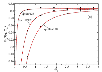
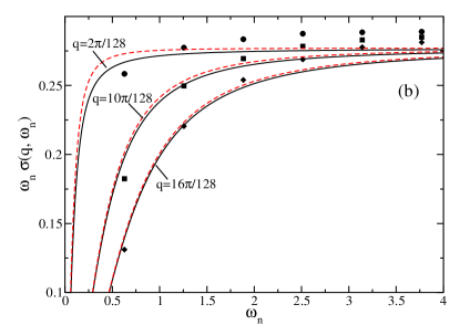
Figure 7: QMC data (symbols) for $T/J=0.1$ and a system size $L=128$ for (a) $\Delta=1/2$, and (b) $\Delta=1$.Alvarez and Gros (2008) In comparison, the field theory result in Eq. (36) (solid lines) and the result obtained by setting $\gamma=0$ (dashed lines) is shown. For $\Delta=1/2$ both cases are almost indistinguishable. For $\Delta=1$ and small $q$ the effect of $\gamma$ is largest, however, in this case also the finite size corrections are large so that a detailed analysis seems very difficult.

In addition we also show the result that is obtained by setting $\gamma=0$ in Eq. (36), corresponding to the BA solution in Ref. [Benz et al., 2005]. Since the agreement is good for both $\gamma=0$ and $\gamma\neq 0$ as given by Eq. (II.2), we conclude that these QMC calculations are not of sufficient accuracy to decide whether or not the relaxation rate vanishes in the integrable model. A general problem in QMC calculations is that a relaxation rate much smaller than the separation between Matsubara frequencies, $\gamma\ll\omega_{n+1}-\omega_{n}=2\pi T$, cannot be resolved.

Promising seems to be a study of the Heisenberg point, where $\gamma(T)\sim T/\ln^{2}(J/T)$ is largest. Indeed, evidence for a nonzero relaxation rate for this case has been found in a very recent QMC study by directly comparing with our result (36) transformed to Matsubara frequencies.Grossjohann and Brenig (2010) The magnitude of $\gamma$ seemed to be roughly consistent with the value in Eq. (II.2). However, as has been already shown in Ref. [Sirker et al., 2009] by comparing with numerical results for the correlation function $C(t)$, logarithmic correction at the isotropic point limit the temperature range where the field theory results are applicable. In QMC calculations a further problem at $\Delta=1$ is the slow logarithmic decay of finite size corrections. It would therefore be desirable to perform a similar study for $\Delta\sim 0.6-0.8$ where $\gamma$ is still fairly large and the field theory seems to work well up to temperatures of the order $T/J\sim 0.2$ as we demonstrated in the previous section and in Ref. [Sirker et al., 2009].

II.6 Spin diffusion

So far we have used our result for the self-energy of the bosonic propagator to discuss the transport properties of the spin chain. In this and the following sections we will discuss diffusive properties characterized by the long-time behavior of the spin-spin correlation function $\langle S_{l+x}^{z}(t)S^{z}_{l}(0)\rangle$. We concentrate again on the case of zero field. For $T=0$, it is knownPereira et al. (2008) that the slowest decaying term in the autocorrelation function for $0<\Delta<1$ is of the form

$$\langle S_{l}^{z}(t)S^{z}_{l}(0)\rangle\sim\frac{e^{-iWt}}{t^{\eta}},\quad(T=0)$$ (59)

with $W=v$ and $\eta=(K+1)/2$. This oscillating term is attributed to $q=\pi/2$ high-energy particle-hole excitations with a hole near the bottom of the band and a particle at the Fermi surface, or a particle at the top of the band and a hole at the Fermi surface. At $T=0$, the low-energy contributions to the spin-spin correlation function decay faster than the high-energy contributions. In contrast, numerical studies seem to suggest that at high temperatures the oscillating terms are still present, but the slowest decaying term has pure power-law decay with no oscillations Fabricius and McCoy (1998); Sirker (2006). This slowly decaying term has been interpreted as due to spin diffusion at high temperatures. Here we will show that a diffusive term is already present at low temperatures. In the following we use the boson propagator in Eq. (20),  (24) to calculate the $q\sim 0$ low-energy contribution to the autocorrelation function in the regime $T\ll J$.

We can write the low-energy, long-wavelength contribution to $\langle S_{l+x}^{z}(t)S^{z}_{l}(0)\rangle$ as

$$G(x,t)\equiv-2\int_{-\infty}^{+\infty}\frac{d\omega}{2\pi}\int_{-\infty}^{+\infty}\frac{dq}{2\pi}\,e^{i(qx-\omega t)}\frac{{\rm Im}\chi_{\rm ret}(q,\omega)}{1-e^{-\omega/T}},$$ (60)

with $\chi_{\rm ret}(q,\omega)$ given by Eq. (20) and (24) . Note that the $-b\omega^{2}$ and $cv^{2}q^{2}$ terms in the self-energy simply rescale the energy and wave-vector by $(1+b)$ and $(1+c)$ respectively, giving a $T$-dependent velocity, $\tilde{v}\equiv\sqrt{(1+c)/(1+b)}v$. Doing the integral over $q$ first, we find (see appendix A for details)

$$\!\!\!\!\!\!\!\!\!\!\!\!\!G(x,t) = \frac{K}{2\pi v^{2}}(1+b)^{-\frac{1}{2}}(1+c)^{-\frac{3}{2}}\int_{-\infty}^{+\infty}\frac{d\tilde{\omega}}{4\pi}\,\exp[-i\tilde{\omega}\tilde{t}-i(\tilde{\omega}^{2}+2i\tilde{\gamma}\tilde{\omega})^{1/2}|\tilde{x}|/v]\,\frac{(\tilde{\omega}^{2}+2i\tilde{\gamma}\tilde{\omega})^{1/2}}{1-e^{-\tilde{\omega}/\tilde{T}}}-(\tilde{\gamma}\to-\tilde{\gamma}),$$ (61)

where $\tilde{t}=t(1+b)^{-1/2}$, $\tilde{x}=x(1+c)^{-1/2}$, $\tilde{\gamma}=\gamma(1+b)^{-1/2}$ and $\tilde{T}=T(1+b)^{1/2}$. The integral in Eq. (61) has both pole and branch cut contributions, inside the light cone when $|t|>\tilde{v}|x|$, but only the pole contribution outside the light cone when $|t|<\tilde{v}|x|$. While this integral could be evaluated more generally numerically, we focus on a couple of simple regions where we can obtain analytic results. One of these is $|x|/v\lll 1/\gamma\ll t$ where

$$G(x,t)=(1+b)^{-1/2}(1+c)^{-3/2}[G_{0}(x,t)+G_{\rm int}(x,t)],$$ (62)

with

$$G_{0}(x,t) = \frac{K}{8\pi^{2}v^{2}}\left\{\frac{\pi\tilde{T}}{\sinh[\pi\tilde{T}(\tilde{t}-\tilde{x}/v)]}\right\}^{2}$$

$$+ \frac{K}{8\pi^{2}v^{2}}\left\{\frac{\pi\tilde{T}}{\sinh[\pi\tilde{T}(\tilde{t}+\tilde{x}/v)]}\right\}^{2}$$

is the Luttinger liquid result in terms of the rescaled variables and

$$G_{\rm int}(x,t)=\frac{K\tilde{T}}{v^{2}}\sqrt{\frac{\gamma}{2\pi t}}\,e^{-\gamma\tilde{x}^{2}/2v^{2}\tilde{t}}$$ (64)

is the diffusive term. The other simple region is $|t|<|x|/v\ll 1/\gamma$ where we just obtain the Luttinger liquid result, $G_{0}$. Note that even for the static correlation function there are for $|x|/v\gtrsim 1/\gamma$ in principle $\gamma$-dependent corrections to the approximately exponential decay (see appendix A). However, since $1/\gamma\gg\xi$ where $\xi=v/(2\pi T)$ is the correlation length, these corrections occur in a regime where the correlation function is already extremely small and where also higher order corrections to (II.6) have to be taken into account. A schematic representation of the behavior expected in the different regions is shown in Fig. 8.

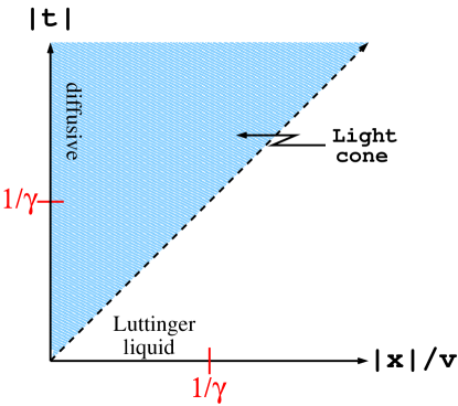
Figure 8: The low-energy, long-wavelength contributions to $\langle S^{z}_{l+x}(t)S^{z}(0)\rangle$ at finite temperatures in different regions of the spacetime diagram. Inside the light cone, Eq. (61) has both branch cut and pole contributions but only pole contributions outside the light cone. The Luttinger liquid result is valid for $|t|<|x|/v\ll 1/\gamma$ whereas the diffusive term (64) dominates for $|x|/v\lll 1/\gamma\ll t$.

We expect these results to be universally valid at large $x$ and $t$, ignoring a possible Drude weight term, since the Fourier transform is dominated by the small $\omega$ and $q$ region, at large $t$ and $x$. $G_{\rm int}$ has the classic diffusion form. Note that diffusion occurs in a more limited domain than originally proposed for high-$T$ ferromagnetsBloembergen (1949); de Gennes (1958); Steiner et al. (1976) however. We have shown it to occur at low $T$, where $\gamma\ll T$, ignoring a possible non-zero Drude weight term in the self-energy, but only inside the light cone at $|x|/v\ll 1/\gamma\ll|t|$ and only for the uniform part of the spin correlation function. (There is also a power-law oscillating term.) Importantly, the domain where classical diffusive behavior occurs does include the self-correlation function. For all $0<\Delta\leq 1$, at finite temperatures and sufficiently long times the autocorrelation function becomes dominated by a low-energy term

$$\langle S_{l}^{z}(t)S^{z}_{l}(0)\rangle\sim T\sqrt{\frac{\gamma(T)}{t}},\quad(T\neq 0,t\gg 1/\gamma)$$ (65)

with the universal power-law decay $t^{-1/2}$ expected for diffusion in one dimension.Bloembergen (1949); de Gennes (1958); Steiner et al. (1976) Note that the more limited diffusive behavior we have found is related to the Lorentz invariance of the underlying low energy effective Lagrangian. The $b$ and $c$ terms break Lorentz invariance but only produce an unimportant$T$-dependent shift of the velocity. The important breaking of Lorentz invariance, which leads to diffusion, is due to the finite temperature. While diffusive behavior occurs only in a limited space-time domain, it is sufficient to give diffusive behavior in certain NMR experiments, as we show in the next sub-section.

II.7 Spin-lattice relaxation rate

If the $q\sim 0$ contribution dominates the dynamics, diffusive behavior should show up as characteristic frequency and magnetic field dependence in NMR experiments. Before deriving a prediction for the spin-lattice relaxation rate based on the results from the previous section and comparing with experiment, we first want to point out a general relation useful to take the finite magnetic field in NMR experiments into account properly.

The linear response formula for the spin-lattice relaxation rate isMoriya (1956)

$$\frac{1}{T_{1}}=\frac{1}{2}\int\frac{dq}{2\pi}\,|A(q)|^{2}S^{+-}(q,\omega_{N})|_{h},$$ (66)

where $A(q)$ is the hyperfine coupling form factor, $\omega_{N}$ is the nuclear magnetic resonance frequency and

$$S^{+-}(q,\omega)|_{h}=\frac{1}{N}\sum_{l,l^{\prime}}\int_{-\infty}^{+\infty}dt\,e^{i\omega_{N}t}\langle S_{l}^{+}(t)S_{l^{\prime}}^{-}(0)\rangle|_{h}$$ (67)

is the transverse dynamical spin structure factor. Here $S^{\pm}_{l}=S^{x}_{l}\pm iS^{y}_{l}$ are the raising and lowering spin operators. The expression in Eq. (67) is to be calculated using Hamiltonian (4) in the presence of a magnetic field $h$. We focus on the experimentally relevant Heisenberg point $\Delta=1$. We would like to express $1/T_{1}$ in terms of the longitudinal structure factor

$$S^{zz}(q,\omega)=\frac{1}{N}\sum_{l,l^{\prime}}\int_{-\infty}^{+\infty}dt\,e^{i\omega_{N}t}\langle S_{l}^{z}(t)S_{l^{\prime}}^{z}(0)\rangle$$ (68)

at zero field. The latter is more easily calculated in the field theory since $S^{z}_{l}$ is related to the local density of fermions $n_{l}$, whereas $S_{l}^{\pm}$ have nonlocal representations in terms of Jordan-Wigner fermions. Although the exchange term in the Heisenberg model is isotropic, the magnetic field term in Eq. (4) breaks rotational symmetry. As a result, $S^{+-}(q,\omega)|_{h}$ cannot be directly replaced by $2S^{zz}(q,\omega)|_{h}$ at finite field. However, we note that the longitudinal field has a trivial effect on $S_{l}^{\pm}(t)$

$$S^{\pm}_{l}(t)=e^{iHt}S_{l}^{\pm}e^{-iHt},=e^{-i\omega_{e}t}e^{i\bar{H}t}S_{l}^{\pm}e^{-i\bar{H}t},$$ (69)

where $\bar{H}=H(h=0)$ and $\omega_{e}=\mu_{B}h$ is the electron magnetic resonance frequency. If we assume in addition that $T\gg\omega_{e}$, the magnetic field dependence in the thermal average can be neglected and we have

$$S^{+-}(q,\omega)|_{h}\approx\frac{2}{N}\sum_{l,l^{\prime}}\int_{-\infty}^{+\infty}dt\,e^{i(\omega_{N}-\omega_{e})t}\langle S_{l}^{z}(t)S_{l^{\prime}}^{z}(0)\rangle|_{0},$$ (70)

where the correlation function is calculated at $h=0$. This leads to the expression for the spin-lattice relaxation rate

$$\frac{1}{T_{1}}\approx\int\frac{dq}{2\pi}\,|A(q)|^{2}S^{zz}(q,\omega_{N}-\omega_{e})|_{0}.$$ (71)

Using $\omega_{e}\gg\omega_{N}$ and

$$S^{zz}(q,-\omega_{e})=\frac{2\,\textrm{Im }\chi_{\rm ret}(q,\omega_{e})}{1-e^{\omega_{e}/T}},$$ (72)

we find in the regime $\omega_{e}\ll T$

$$\frac{1}{T_{1}}\approx-\frac{2T}{\omega_{e}}\int\frac{dq}{2\pi}\,|A(q)|^{2}\textrm{Im }\chi_{\rm ret}(q,\omega_{e}).$$ (73)

If the integral in Eq. (73) is dominated at low temperatures, $T\ll J$, by the $q\sim 0$ mode of $\chi_{\rm ret}(q,\omega)$ then we can perform the momentum integral using the retarded correlation function in Eq. (20). Assuming furthermore that the momentum dependence can be neglected, $A(q\sim 0)\equiv A=\mbox{const}$, and using the appropriate parameters (II.2) for the isotropic case we find

$$\frac{1}{T_{1}T}=2|A|^{2}X_{1}\sqrt{\frac{X_{2}}{2}+\sqrt{\left(\frac{X_{2}}{2}\right)^{2}+\left(\frac{\gamma}{\omega_{e}}\right)^{2}}},$$ (74)

where

$$X_{1} = 1+\frac{g}{2}-\frac{g^{2}}{8}+\frac{5g^{3}}{64}+\frac{3\sqrt{3}}{2\pi}T^{2},$$

$$X_{2} = 1+\frac{g^{2}}{4}-\frac{g^{3}}{32}\left(3-\frac{8\pi^{2}}{3}\right)+\frac{\sqrt{3}}{\pi}T^{2}.$$ (75)

In the limit $\gamma(T)\gg\omega_{e}$, we obtain the diffusive behavior

$$\frac{1}{T_{1}T}\sim\sqrt{\frac{\gamma(T)}{\omega_{e}}}\sim\sqrt{\frac{T/\ln^{2}(J/T)}{\omega_{e}}}.$$ (76)

In the NMR experiment by Thurber et al., Ref. [Thurber et al., 2001], the copper-oxygen spin chain compound Sr₂CuO₃ was studied. In this compound an in-chain oxygen site exists such that $A(q)=A\cos(q/2)$ in (73). In NMR measurements on this oxygen site any contribution to the spin-lattice relaxation rate coming from $q\sim\pi$ is therefore almost completely suppressed so that the $q\sim 0$ mode dominates. Note that for NMR measurements on the copper or the apical oxygen site both low-energy contributions would be present with the $q\sim\pi$ being dominant. In Ref. [Thurber et al., 2001] the experimental data for the in-chain oxygen site have been interpreted in terms of a spin-lattice relaxation rate $1/T_{1}T\sim T/\sqrt{\omega_{e}}$. While the frequency dependence does agree with that found in Eq. (76) and generally expected if diffusion holds, we note that the temperature dependence of the effective diffusion constant $D_{s}\equiv v^{2}/2\gamma$ is different.

To quantitatively compare our prediction with experiment we note that the form factor $A(q)=A\cos(q/2)$ for the in-chain oxygen site is given by

$$|A|^{2}=\frac{k_{B}}{2\hbar}\frac{(2C^{b})^{2}+(2C^{c})^{2}}{\pi^{3}k_{B}^{2}J^{2}}(g\gamma_{N}\hbar)^{2},$$ (77)

where $k_{B}$ is the Boltzmann constant, $C^{b,c}$ are the dimensionless components of the hyperfine coupling tensor, $g\gamma_{N}\hbar=4.74\times 10^{-9}$ eV and $J$ is the exchange coupling measured in Kelvin. The components of the hyperfine coupling tensor can be obtained by performing a $K-\chi$ analysis, i.e., a comparison between measurements of the Knight shift $K$ and the magnetic susceptibility $\chi$. Such an analysis has been performed in Ref. [Thurber et al., 2001] leading to $2C^{b}=95\pm 10$ and $2C^{c}=44\pm 10$ kOe/$\mu_{B}$. Furthermore, the exchange coupling $J$ has to be determined. We note that a parameter-free field theory formula for the static magnetic susceptibility follows from

$$\chi = -\chi_{\rm ret}(q,0)=\frac{K}{2\pi v}\frac{1}{1+c}$$

$$\approx \frac{1}{\pi^{2}}\left[1+\frac{g}{2}+\frac{3g^{3}}{32}+\frac{\sqrt{3}}{\pi}T^{2}\right]$$

where we have used Eqs. (20, 24). In the second line, we have specialized for the isotropic point, with $v=\pi/2$, $K\to 1+g/2+g^{2}/4+g^{3}/8$, and the parameter $c$ as given in (II.2). Eq. (II.7) is in agreement with the result in Refs. [Lukyanov, 1998; Sirker et al., 2008]. Using this formula and fitting the susceptibility data in Ref. [Motoyama et al., 1996] we obtain $J=2000\pm 200$ K. In Fig. 9 the shaded area denotes the region covered by the curves obtained by varying the parameters $J$ and $C^{b,c}$ independently within the given range. However, if we believe that the field theory describes the zero temperature limit correctly then the possible variation of the theoretical results is strongly overestimated. From Eq. (74) we see that $1/(T_{1}T)\to 2|A|^{2}$ for $T\to 0$ and is therefore not affected by the question how large $\gamma$ is. For a given $J$ we can therefore fix $(2C^{b})^{2}+(2C^{c})^{2}$ in (77) by fitting the experimental data at low temperatures. The remaining variation is then very small (see the two examples in Fig. 9).

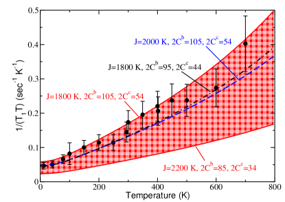
Figure 9: Experimental data for the spin-lattice relaxation rate of the spin chain compound Sr₂CuO₃ at $h=9$ T taken from Ref. [Thurber et al., 2001] (dots) compared to our theory. The solid lines represent the two extreme limits when varying $J$, $C^{b,c}$ independently within the given error bars. The other two curves correspond to fixing the hyperfine constants for a given $J$ by the experimental data at low temperatures.

For $\gamma=0$ corresponding to purely ballistic transport, as suggested by the Bethe ansatz calculation of Ref. [Benz et al., 2005], $1/(T_{1}T)$ would be approximately constant.Sirker et al. (2009) Further support that the good agreement seen in Fig. 9 is not accidental is obtained by an analysis of the NMR data for the apical oxygen site which is also presented in Ref. [Thurber et al., 2001]. In this case the hyperfine coupling tensor $A(q)$ is momentum independent and the contribution from low-energy excitations with $q\sim\pi$ dominates. In this case field theory yieldsSachdev (1994)

$$\frac{1}{T_{1}}=\frac{(D^{b})^{2}+(D^{c})^{2}}{(2\pi)^{3/2}}\frac{(g\gamma_{N}\hbar)^{2}}{\hbar k_{B}J}$$ (79)

with $D^{b}=23\pm 10$ and $D^{b}=14\pm 10$ kOe/$\mu_{B}$.Thurber et al. (2001) Using again $J=2000$ K the experimental data in Ref. [Thurber et al., 2001] are very well described by this formula. Therefore the experimental data for the magnetic susceptibility and the NMR relaxation rates, testing the low-energy contributions of $\chi_{\rm ret}(q,\omega)$, both at $q\sim 0$ and $q\sim\pi$, are consistently described using $J\sim 2000$ K and a hyperfine coupling tensor as determined experimentally by a $K-\chi$ analysis.

II.8 Consequences for electron spin resonance

Here we want to point out a connection between our study of the conductivity of the $S=1/2$ Heisenberg chain and a previous theory of electron spin resonance (ESR) for such systems.Oshikawa and Affleck (1997) By also using a self-energy approach for the boson propagator it was shown in this work that the ESR lineshape is Lorentzian with a width given by the imaginary part of the retarded self-energy. In particular, the case of an exchange anisotropy perpendicular to the applied magnetic field was considered. In this case the ESR linewidth for an applied magnetic field $h$ is given by

$$\eta=-\mbox{Im}\,\Pi_{u}^{\rm ret}(h,h)/(2h)$$ (80)

where $\Pi_{u}^{\textrm{ret}}(h,h)$ is the retarded self-energy due to Umklapp scattering, Eq. (21), for the isotropic case. From (24) and (II.2) we therefore immediately obtain

$$\eta\equiv\gamma=\frac{\pi}{2}g^{2}T.$$ (81)

This is consistent with Eq. (6.27) in Ref. [Oshikawa and Affleck, 1997] using the standard replacement $\lambda\to g/4$ in reverse and in addition $\lambda\to v\lambda$ with $v=\pi/2$ because in [Oshikawa and Affleck, 1997] the spin velocity was set to $1$. The RG flow for the running coupling constant $g$ is now cut off by the larger of the temperature $T$ or the applied magnetic field $h$. If these two scales are sufficiently different, we can use Eq. (28) for $g$ with $T$ being replaced by $\mbox{max}(T,h)$. In this case (81) is a parameter-free prediction for the ESR linewidth of a $S=1/2$ Heisenberg chain with a small exchange anisotropy perpendicular to the applied magnetic field.

We want to stress that a vanishing relaxation rate $\gamma$ would dramatically affect the ESR linewidth. From (21) and (II.2) we obtain for $\omega/T,\,q/T\ll 1$

$$\Pi_{u}^{\rm ret}(q,\omega) \sim F^{\rm ret}(q,\omega)-F^{\rm ret}(0,0)$$

$$\sim \omega^{2}+q^{2}+\frac{q^{2}\omega^{2}}{T^{2}}+\text{i}\left(2\gamma\omega+\frac{q^{2}\omega}{T}\right).$$

This leads to

$$\eta=-\mbox{Im}\,\Pi_{u}^{\rm ret}(h,h)/(2h)\sim\gamma+h^{2}/T$$ (83)

and therefore a linewidth $\eta\sim h^{2}/T$ if $\gamma=0$.

II.9 Consequences for the spin structure factor

The longitudinal dynamical spin structure factor at finite temperatures can be obtained from

$$S^{zz}(q,\omega)=-\frac{2}{1-\text{e}^{-\beta\omega}}\mbox{Im}\,\chi^{\textrm{ret}}(q,\omega)$$ (84)

In the low-energy, long-wavelength limit the retarded spin-spin correlation function can be again expressed by the boson propagator using Eq. (20). With the help of (33) we therefore obtain a direct relation between the spin structure factor and the real part of the conductivity

$$S^{zz}(q,\omega)=\frac{2q^{2}}{\omega(1-\text{e}^{-\beta\omega})}\sigma^{\prime}(q,\omega)\quad(q\ll 1).$$ (85)

>From (37) we see that our theory predicts a Lorentzian lineshape at finite temperatures. For $T\to 0$ the parameters $b,c,\gamma$ in (37) vanish and we find the well-known free boson result $2S^{zz}(q,\omega)=K|q|\delta(\omega-v|q|)$.

Here some comments are in order. In our perturbative calculation we have only included the band curvature terms to first order. While the lowest order contribution vanishes at zero temperature, the terms of order $2n$ show divergencies on shell, $\omega\sim vq$.Pereira et al. (2007) While it is not yet clear how to sum up a series of such terms, we know from BABougourzi et al. (1998) that they lead to a finite linewidth $\delta\omega(q)\sim q^{3}$ at zero temperature. The lineshape at zero temperature is distinctly non-Lorentzian with threshold singularities. For finite temperature such that $\gamma(T)\gg\delta\omega(q)$ we can, however, neglect these terms and Eq. (85) becomes valid. Furthermore, we note that the second order Umklapp contribution to the self-energy leads for zero temperature to the high-frequency tail of $S^{zz}(q,\omega)$ given in Eq. (7.24) of Ref. [Pereira et al., 2007]. From Eq. (85) it is also clear that the regular part of the conductivity and a part which could possibly yield a ballistic channel for dc transport are not independent but rather have to fulfill sum rules, as for example, $\int d\omega S^{zz}(q,\omega)=2\pi\sum_{j}\exp(\text{i}qj)\langle S_{j}(0)S_{0}(0)\rangle$. The right hand side of this sum rule can be calculated numerically with high accuracy since it only involves static correlation functions.

III Haldane-Shastry model

Unlike the $XXZ$ model, generic spin models with exchange interactions beyond nearest neighbor are not integrable. Here we want to consider a special spin model with long-range interactions that is known to be integrable, even though it is not solvable by Bethe ansatz. The Haldane-Shastry model is given by

$$H=\sum_{j<l}J_{jl}\mathbf{S}_{j}\cdot\mathbf{S}_{l},$$ (86)

where $J_{jl}=J(j-l)=\{(L/\pi)\sin[\pi(j-l)/L]\}^{-2}$ is the long-range exchange interaction.Haldane (1988); Shastry (1988) For a chain with size $L$ and periodic boundary conditions, $J_{jl}$ is inversely proportional to the square of the chord distance between sites $j$ and $l$. We set the energy scale of the exchange interaction such that in the thermodynamic limit $J_{jl}\to(j-l)^{-2}$.

The Haldane-Shastry model is completely integrable as the transfer matrix satisfies the Yang-Baxter equation. The conserved quantities are nonlocal and are not obtained by the traditional method of expanding the transfer matrix. However, they have been found using the “freezing trick” starting from the SU(2) Calogero-Sutherland model.Talstra and Haldane (1995) The exact spectrum is given by the dispersion of free spinons, which contrasts with the interacting spinons of the Heisenberg model. The dynamical structure factor has been calculated exactly.Talstra and Haldane (1994) It has a square-root singularity at the lower threshold of the two-spinon continuum, as expected for SU(2) symmetric models. Contrary to the Heisenberg model, there are no multiplicative logarithmic corrections to the asymptotic behavior of correlation functions. This means that in the effective field theory for the Haldane-Shastry model the coupling constant of the umklapp operator is fine tuned to zero.

Since the umklapp operator is responsible for the leading decay process of the spin current in the calculation in Sec. II.3, we may expect that spin transport in the Haldane-Shastry model is purely ballistic. This seems reasonable given the picture of an ideal spinon gas, but requires that the coupling constants of all higher order Umklapp processes also vanish exactly.

Although the total spin is conserved, the spin density does not satisfy a local continuity equation due to the long-range nature of the exchange interactions. Nonetheless, the spin current operator can be defined using the equivalence to a model of spinless fermions coupled to an electromagnetic field. In terms of Jordan-Wigner fermions, the Haldane-Shastry model reads

$$H = \sum_{j<l}J_{jl}\left[\left(n_{j}-\frac{1}{2}\right)\left(n_{l}-\frac{1}{2}\right)\right.$$ (87)

$$\left.+\frac{(-1)^{l-j}}{2}\left(c_{j}^{\dagger}e^{i\pi\sum_{p=j}^{l-1}n_{p}}c^{\phantom{\dagger}}_{l}+h.c.\right)\right].$$

We then consider a magnetic flux $\Phi$ that threads the chain and couples to the fermionic fields in the form $c_{j}^{\dagger}c^{\phantom{\dagger}}_{l}\to c_{j}^{\dagger}c^{\phantom{\dagger}}_{l}e^{-i\sum_{m=j}^{l-1}A_{m,m+1}}$. Here $A_{m,m+1}$ is the vector potential defined on the link between sites $m$ and $m+1$, such that $\sum_{m=1}^{N}A_{m,m+1}=\Phi$. The Hamiltonian in the presence of the electromagnetic field becomes

$$H = \sum_{j<l}J_{jl}\left[\left(n_{j}-\frac{1}{2}\right)\left(n_{l}-\frac{1}{2}\right)\right.+\frac{(-1)^{l-j}}{2}\times$$ (88)

$$\left.\times\left(c_{j}^{\dagger}e^{i\sum_{p=j}^{l-1}(\pi n_{p}-A_{p,p+1})}c^{\phantom{\dagger}}_{l}+h.c.\right)\right].$$

The current operator associated with a given link is defined as

$$\mathcal{J}_{j,j+1} = -\frac{\partial H}{\partial A_{j,j+1}}$$

$$= \frac{i}{2}\sum_{n>0}\sum_{\ell=0}^{n-1}(-1)^{n}J(n)\>\times$$

$$\times c_{j-\ell}^{\dagger}e^{i\sum_{p=j-\ell}^{j-\ell+n-1}(\pi n_{p}-A_{p,p+1})}c^{\phantom{\dagger}}_{j-\ell+n}$$

$$+h.c..$$

Therefore the integrated current operator in the limit of weak fields, $A_{j,j+1}\to 0$, reads

$$\mathcal{J} = \sum_{j}\mathcal{J}_{j,j+1}$$

$$= \frac{i}{2}\sum_{j}\sum_{n\neq 0}(-1)^{n}nJ(n)c_{j}^{\dagger}e^{i\pi\sum_{p=j}^{j+n-1}n_{p}}c^{\phantom{\dagger}}_{j+n}.$$

Reverting to spin operators, we obtain the spin current operator

$$\mathcal{J}=\frac{i}{2}\sum_{j}\sum_{n\neq 0}nJ(n)S_{j}^{+}S_{j+n}^{-}.$$ (91)

Notice that $\mathcal{J}$ is a nonlocal operator, since it acts on sites separated by arbitrary distances.

We can now compute the commutator of the current operator with the Hamiltonian in Eq. (86). The result is

$$[\mathcal{J},H] = \frac{i}{2}\sum_{l\neq m\neq n}[(m-n)J_{mn}(J_{ln}-J_{lm})$$ (92)

$$+(2l-m-n)J_{lm}J_{ln}]S_{l}^{z}S_{m}^{+}S_{n}^{-}.$$

In the thermodynamic limit, $J(n)\to 1/n^{2}$ and we find

$$[\mathcal{J},H]=0.$$ (93)

Therefore, the current operator is conserved and transport is ballistic in the thermodynamic limit. That the conservation law does not hold for a finite chain can be easily seen by considering a three site ring. In this case the Hamiltonian and current operator of the Haldane-Shastry model reduce to those of the Heisenberg model, and these two operators clearly do not commute.

The current operator is orthogonal to the set of conserved quantities associated with integrability. For instance, the first nontrivial conserved quantity is

$$Q_{3}=i\sum_{ijk}\frac{z_{i}z_{j}z_{k}}{z_{ij}z_{jk}z_{ki}}\mathbf{S}_{i}\cdot(\mathbf{S}_{j}\times\mathbf{S}_{k}),$$ (94)

where $z_{j}=e^{i2\pi j/L}$ and $z_{ij}=z_{i}-z_{j}$. The orthogonality can be shown by arguing that the current operator is odd under a $\pi$ rotation about the $x$ axis, which takes $S^{z}_{j}\to-S^{z}_{j}$ and $S^{y}_{j}\to-S^{y}_{j}$, whereas the conserved quantities derived in Ref. [ Talstra and Haldane, 1995] are SU(2) invariants and therefore even under this transformation. Unlike the current operator, these conserved quantities commute with the Hamiltonian for a finite chain with periodic boundary conditions.

IV The attractive Hubbard model

We now want to consider the negative $U$ Hubbard model at 1/2-filling

$$H=\sum_{j}[-(c^{\dagger}_{\alpha j}c_{\alpha j+1}+h.c.)-U(\hat{n}_{j}-1/2)^{2}].$$ (95)

We may take the continuum limit and bosonize the resulting Dirac fermions, which now carry a spin index, finally introducing charge and spin bosons. These are decoupled up to irrelevant operators. For $U<0$ and zero magnetic field, the spin excitations are gapped and we expect the associated contribution to the low frequency conductivity to be Boltzmann suppressed at temperatures small compared to the spin gap. The low energy effective Hamiltonian contains only the charge boson, which we again call $\phi$ for simplicity. This low-energy Hamiltonian now contains the Umklapp scattering term

$$H_{u} = \tilde{\lambda}\int dx\left[\psi^{\dagger}_{L\uparrow}\psi^{\dagger}_{L\downarrow}\psi_{R\uparrow}\psi_{R\downarrow}+h.c.\right]$$ (96)

$$= \lambda\int dx\cos(\sqrt{8\pi}\phi).$$

The bare coupling constant $\lambda$ is $\propto-U$ at small $U$. It is marginally irrelevant, as in the spinless model at $\Delta=1$, and the effective coupling at scale $T$ behaves similarly to Eq. (28)

$${1\over\lambda(T)}+{\ln\lambda(T)\over 2}=\ln\left[{T_{0}\over T}\right]$$ (97)

where the cut-off scale $T_{0}$ depends on $U$. Thus the self-energy for the charge boson has the form of Eq. (24), with

$$2\gamma(T)=\pi\lambda^{2}(T)T$$ (98)

as in Eq. (II.2).

This lowest order, RG improved, calculation again ignores the possibility of a Drude weight. A rigorous Mazur bound on the Drude weight for the Hubbard model was established in [Zotos et al., 1997], using the conserved energy current, but it fails at half-filling where $\langle\mathcal{J}\mathcal{J}_{E}\rangle=0$. In this case, other local conserved charges have not been considered.

In the limit $U/t\to-\infty$, the spin gap becomes infinite and the model is equivalent to the Heisenberg model with $J\propto t^{2}/U$ and charge operators replacing spin operators. In this limit, we may import all results discussed above for the Heisenberg model. The fact that the Hubbard interaction is marginal ($K=1$), as well as the equivalence with the Heisenberg model at large $U$ follow from the exact duality transformation

$$c_{\uparrow j} \to (-1)^{j}c^{\dagger}_{\uparrow j}$$

$$c_{\downarrow j} \to c_{\downarrow j}$$ (99)

which changes the sign of $U$. This maps bilinear operators as follows

$$\hat{n}^{j} \to 2S^{z}_{j}$$

$$\hat{c}^{\dagger}_{j,\alpha}c_{j+1,\alpha}-h.c. \to -(c^{\dagger}_{j}\sigma^{z}c_{j+1}-h.c.).$$ (100)

The charge current maps into the spin current. Adding a chemical potential to dope away from 1/2-filling at negative $U$ is equivalent to adding a magnetic field at positive $U$. In the large negative $U$ limit, where we only allow empty sites and double occupancy, this becomes equivalent to the Heisenberg model ($\Delta=1$). The spin SU(2) symmetry of the $U>0$ model implies a “hidden” SU(2) symmetry in the charge sector. Thus, the Hubbard model at half-filling actually has $SU(2)\times SU(2)/Z_{2}=SO(4)$ symmetry for either sign of $U$.

The continuum limit model also has a duality symmetry

$$\psi_{L/R\uparrow}(x) \to \psi_{L/R\uparrow}^{\dagger}(x)$$

$$\psi_{L/R\downarrow}(x) \to \psi_{L/R\downarrow}(x).$$ (101)

Umklapp at $U<0$ maps into the $\pm$ component of the marginal spin operator at $U>0$:

$$\psi^{\dagger}_{L\downarrow}\psi^{\dagger}_{L\uparrow}\psi_{R\uparrow}\psi_{R\downarrow}\to\psi^{\dagger}_{L\downarrow}\psi_{L\uparrow}\psi^{\dagger}_{R\uparrow}\psi_{R\downarrow}.$$ (102)

Similarly, the product of left and right charge currents maps into the product of left and right z-components of spin currents: $J_{L}J_{R}\to 4J^{z}_{L}J^{z}_{R}$. There is an exact $SU(2)\times SU(2)$ symmetry of the continuum model. Umklapp and $J_{L}J_{R}$ interactions are sitting exactly on the separatrix of the Kosterlitz-Thouless RG flow.

We might think of a negative $U$ as arising from phonon exchange. More general models, with longer range interactions will not be on the separatrix but may have the low energy Hamiltonian, with Umklapp and $J_{L}J_{R}$ interactions. For a range of interaction parameters, the Umklapp will be irrelevant and we get a Lorentzian conductivity.

The negative $U$ Hubbard model may be thought of as being in a one-dimensional version of a superconducting state. However, it is important to realize that it is not a true superconductor and the presence or absence of a finite Drude weight at finite $T$ is independent of the absence of true superconductivity. One way of seeing this point is to consider a ring of circumference $L$ penetrated by a flux $\Phi$. If the ring was a torus of sufficiently large thickness, we might be able to model its properties using London theory. Using the London equation

$$\boldsymbol{j}=-{n_{s}(e^{*})^{2}\over mc}\boldsymbol{A}$$ (103)

and $A=\Phi/L$, we obtain a persistent current $\propto 1/L$

$$j=-{n_{s}(e^{*})^{2}\Phi\over mcL}.$$ (104)

Here $e^{*}=2e$ is the charge of the Cooper pairs. In London theory, this formula is true at finite $T$ with $n_{s}(T)$, the superfluid density, a decreasing function of $T$ which is non-zero for $T<T_{c}$. On the other hand, for the one-dimensional Hubbard model, the finite size spectrum for current-carrying states is:

$$E={\pi v_{c}\over L}(n+\Phi/2\pi)^{2}+E_{0}$$ (105)

where $v_{c}$ is the velocity of charge excitations. (This result is obtained ignoring the irrelevant Umklapp interactions.) The partition function is

$$Z=Z_{0}\sum_{n=-\infty}^{\infty}\exp[-(\pi v_{c}/LT)(n+\Phi/2\pi)^{2}],$$ (106)

and the resulting persistent current

$$j=\partial F/\partial\Phi.$$ (107)

For sufficiently large $L$ such that $T$ is much greater than the finite size gap, $T\gg v_{c}/L$, this gives

$$j\approx-2\sin\Phi\sqrt{LT\over v_{c}}e^{-\pi LT/v_{c}}.$$ (108)

This is exponentially small in $L$, unlike the case for a superconductor, Eq. (104). The superfluid density vanishes at any finite $T$. On the other hand, if we ignore Umklapp scattering, the model has a $T$-independent Drude weight $D=v_{c}/4\pi$, as in Eq. (II.3).

>From the London equation for a superconductor it follows that

$$\lim_{\omega\to 0}\omega\ \hbox{Im}\ \sigma(\omega,q)={n_{s}(e^{*})^{2}\over m}$$ (109)

independent of $q$. On the other hand, for the Hubbard model, $\mbox{Im}\,\sigma(q,\omega)$ can be obtained from Eq. (36) with $v\to v_{c}$ and it is easy to see that $\omega\,\mbox{Im}\,\sigma(q,\omega)$ vanishes in the limit $\omega\to 0$ at non-zero $q$.

V Summary and conclusions

To summarize, we have studied how nontrivial conservation laws affect the transport properties of one-dimensional quantum systems. We focused, in particular, on the spin current in the integrable $XXZ$ model. Away from half-filling, a part of the spin current is protected by conservation laws leading to a ballistic channel which coexists with a diffusive channel. For the half-filled case, however, none of the infinitely many local conservation laws responsible for integrability has any overlap with the current by symmetry. Nonetheless, several works have argued in favor of ballistic transport at finite temperatures even in this situation. This would require the existence of an unknown nonlocal conservation law which has finite overlap with the current operator. To investigate this controversial problem, our strategy was the following: Assuming that such a conservation law does not exist, we calculated the current relaxation within the Kubo formalism using a self-energy approach for the boson propagator. Since the parameters in the field theory are explicitly known due to the integrability of the microscopic model we obtained a parameter-free formula for the optical conductivity. Any shift of weight from this regular into a Drude part can then be described within the memory-matrix formalism and explicitly tested for by comparing the parameter-free result with numerical and experimental data.

By a numerical study of the time-dependent current-current correlation function we have shown that the intermediate time decay is well described by the calculated relaxation rate. This excludes, in particular, the large Drude weight found by Bethe ansatz in Ref. [Benz et al., 2005]. As we have shown, this result corresponds to our field theory with the relaxation rate set exactly to zero by hand. A small Drude weight can, however, not be excluded by the intermediate time data. This includes, in particular, the Drude weight found in a different Bethe ansatz calculation.Zotos (1999) At least at high temperatures it is, however, known that this approach violates exact relations so that the solution cannot be exact. It is not clear at present if or why these results could be considered as an approximate solution at low temperatures. Quantum Monte Carlo calculations, on the other hand, are performed using imaginary times. The results presented in Refs. [Alvarez and Gros, 2002a, b] therefore cannot be used to resolve a decay rate smaller than the separation of Matsubara frequencies. An interesting possibility is the idea to analytically continue our results to imaginary frequencies and to check if this is consistent with Quantum Monte Carlo data. Such an analysis has been performed recently for the isotropic case and good agreement was found.Grossjohann and Brenig (2010) It would be very interesting to perform a similar analysis in the anisotropic case for $\Delta$ values such that the decay rate is not too small. The advantage would be that additional complications due to logarithmic corrections present at the isotropic point do not occur. In Ref. [Sirker et al., 2009] we also presented numerical data for the current-current correlation funciton at infinite temperatures and showed that even in this case a large time scale persists. It is therefore unclear how data obtained by exact diagonalization can be reliably extrapolated to the thermodynamic limit.

>From our perturbative result for the boson propagator at finite temperatures we found that the long-wavelength contribution to the spin-lattice relaxation rate is diffusive. By comparing with experiments on the spin chain compound Sr₂CuO₃ we showed that our formula describes the experimental data well. Importantly, we showed that the data for the magnetic susceptibility and the $q\sim 0$ and $q\sim\pi$ contributions to the spin-lattice relaxation rate are all consistently described by the field theory formulas with the same exchange constant $J$ and using the hyperfine coupling tensor as determined experimentally. We also pointed out that our results are consistent with a previous theory of electron spin resonance in spin chainsOshikawa and Affleck (1997). For the longitudinal spin structure factor at zero magnetic field our theory predicts a crossover from the known non-Lorentzian lineshape with linewidth $\sim q^{3}$ at zero temperature, to a Lorentzian lineshape with a linewidth set by the relaxation rate $\gamma$ at sufficiently high temperatures.

We also discussed the integrable Haldane-Shastry model where the spectrum is known to consist of free spinons in contrast to the interacting spinons in the Heisenberg model. As in the Heisenberg model at zero magnetic field the current operator does not have any overlap with the known conserved quantities. However, in this case the nonlocal current operator itself becomes conserved in the thermodynamic limit and transport is therefore ballistic.

Finally, we showed that our calculations for the spin current in the $XXZ$ model carry over to the charge current in the attractive Hubbard model at half-filling. We stressed the point that an infinite dc conductivity does not imply that the system is a true superconductor. This can be seen by calculating the superfluid density which turns out to be zero in this case.

Appendix A Spin Green’s function

Consider a boson propagator with a momentum-independent decay term (see Eq. (20))

$$\chi_{ret}(q,\omega) \equiv -i\int_{0}^{\infty}dt\int_{-\infty}^{\infty}dx$$ (110)

$$\times e^{i(\omega t-qx)}\langle[\partial_{x}\phi(t,x),\partial_{x}\phi(0,0)]\rangle_{T}$$

$$\to {q^{2}\over\omega^{2}-q^{2}+2i\gamma(T)\omega},$$

for small $\omega$ and $q$. (We set the velocity equal to 1. $\gamma$ must be $>0$ by causality.) We wish to calculate the long-time behavior of the correlation function

$$G(x,t)\equiv\frac{K}{2\pi}\langle\partial_{x}\phi(t,x)\partial_{x}\phi(0,0)\rangle_{T},$$ (111)

which can be expressed in terms of $\chi_{ret}(q,\omega)$ with the help of Eq. (60). Using this equation and (110) we find

$$G(x,t)\to-i\int{d\omega dq\over(2\pi)^{2}}{e^{-i(\omega t-qx)}q^{2}\over(1-e^{-\beta\omega})[q-(\omega^{2}+2i\gamma\omega)^{1/2}][q+(\omega^{2}+2i\gamma\omega)^{1/2}]}-(\gamma\to-\gamma).$$ (112)

We now consider only the first term; we return to the $\gamma\to-\gamma$ term later. We are defining $(\omega^{2}+2i\gamma\omega)^{1/2}$ to be a particular branch of the square root; let us specify carefully which one. It will be convenient to define this branch with the branch cut along the negative imaginary $\omega$ axis between $\omega=0$ and $\omega=-2i\gamma$. Thus

$$(\omega^{2}+2i\gamma\omega)^{1/2} \to \sqrt{2\gamma u-u^{2}}\ \ (\omega=-iu+\delta,\ \ 0<u<2\gamma,\ \ \delta\to 0^{+})$$ (113)

$$\to \omega+i\gamma\ \ (|\omega|\gg\gamma)$$

$$\to -\sqrt{2\gamma u-u^{2}}\ \ (\omega=-iu-\delta,\ \ 0<u<2\gamma,\ \ \delta\to 0^{+}).$$

We do the $q$-integral first. Noting that the result is manifestly an even function of $x$, we just consider explicitly the case $x>0$. Noting that this branch of $(\omega^{2}+2i\gamma\omega)^{1/2}$ always has a positive imaginary part for real $\omega$, we may close the $q$ integral in the upper half plane, encircling the pole at $q=(\omega^{2}+2i\gamma\omega)^{1/2}$, giving

$$G_{\hbox{first}}(x,t) \to \int{d\omega\over 4\pi}\exp[-i\omega t+i(\omega^{2}+2i\gamma\omega)^{1/2}|x|]$$ (114)

$$\times {(\omega^{2}+2i\gamma\omega)^{1/2}\over 1-e^{-\beta\omega}}.$$

Consider the analytic structure of the integrand in the complex $\omega$ plane. (We consider only the first term; we return to the $\gamma\to-\gamma$ term later.) There is a branch cut along the negative imaginary axis from $\omega=0$ to $\omega=-2i\gamma$. There are also poles at $\omega=2\pi inT$ for $n=\pm 1$, $\pm 2,\ldots$. The integrand behaves as $1/\omega^{1/2}$ at $\omega\to 0$ so the integral is convergent. Let’s assume $|t|>|x|$. Then, we can close the integral in the upper half plane for $t<0$ or the lower half-plane for $t>0$. First consider the simpler case $t<0$. Then we only pick up the contributions from the poles $\omega=2\pi inT$, $n=1$, $2$, $3,\ldots$ Let us now assume $\gamma(T)\ll T$. Note that we expect this to be true at low $T$, $\gamma(T)\propto T^{4K-3}$, $K>1$. Then, at the poles:

$$(\omega^{2}+2i\gamma\omega)^{1/2}\approx\omega=2\pi inT.$$ (115)

Then, for $t<0$, the first term gives the approximately $\gamma$-independent result:

$$G_{\hbox{first}}^{\,t<0}(x,t)\!\!\! \to \!\!\!-\pi T^{2}\sum_{n=1}^{\infty}n\,e^{2\pi nT(t-\sqrt{1+\gamma/(\pi nT)}|x|)}$$

$$\approx {-e^{-\gamma|x|}\over 4\pi}{1\over\{(1/\pi T)\sinh[\pi T(t-|x|)]\}^{2}}.$$

Actually, while we can always ignore the $\gamma$-dependent corrections to the pre-factor, those corrections in the exponent cannot be ignored at sufficiently large $|x|$. We have Taylor expanded the square root in the exponential to first order in $\gamma/T$. We see that the correction becomes important at $|x|$ of order $1/\gamma$. At such large values of $|x|$, higher order corrections must also be included. If we assume $|x|\ll 1/\gamma$ we may simply drop the $e^{-\gamma|x|}$ factor.

Now consider the first term in Eq. (114) for $t>0$. There are now both pole and cut contributions. For the pole contributions we find again

$$G_{\hbox{first,pole}}^{\,t>0}\to{-e^{-\gamma|x|}\over 4\pi}{1\over\{(1/\pi T)\sinh[\pi T(t-|x|)]\}^{2}}.$$ (117)

But now, we must also consider the cut contribution. We may Taylor expand the denominator in Eq. (114) to first order since $\beta|\omega|\ll 1$ along the cut, $\omega=-iu$, with $0<u<2\gamma\ll T$. Thus:

$$G_{\hbox{first,cut}}^{\,t>0} \to {1\over 4\pi\beta}\int_{0}^{2\gamma}{du\over u}\sqrt{2\gamma u-u^{2}}e^{-ut}$$

$$\!\!\!\!\!\!\!\!\!\!\!\!\!\!\!\!\!\!\!\times \!\!\!\!\!\!\!\!\!\!\!\!\!\!\{\exp[-i\sqrt{2\gamma u-u^{2}}|x|]+\exp[i\sqrt{2\gamma u-u^{2}}|x|]\}.$$

Now let us assume $|t|\gg 1/\gamma$, so that the integral is dominated by $u\ll 1/\gamma$ and we may approximate it by:

$$G_{\hbox{first,cut}}^{\,t>0} \to {1\over 2\pi\beta}\int_{0}^{\infty}du\sqrt{2\gamma\over u}e^{-ut}$$

$$\times \cos\left[\left(\sqrt{2\gamma u}-\frac{u^{3/2}}{2\sqrt{2\gamma}}\right)|x|\right].$$

Here we have expanded the square root to first order in the exponential. This first correction, as well as the higher order ones, may be dropped provided that:

$$|x|\ll|t|\sqrt{\gamma|t|}.$$ (120)

Note that this is automatically true since we have already assumed $|x|<|t|$ and $\sqrt{\gamma|t|}\gg 1$. Assuming Eq. (120) and letting $u=v^{2}/2$, this becomes

$$C_{\hbox{first,cut}}^{\,t>0} \to {\sqrt{\gamma}\over 2\pi\beta}\int_{0}^{\infty}dve^{-v^{2}|t|/2}[e^{-i\sqrt{\gamma}|x|v}+c.c.]$$ (121)

$$= T\sqrt{2\pi\gamma\over|t|}e^{-\gamma x^{2}/(2|t|)}.$$

Now consider the $\gamma\to-\gamma$ term in Eq. (112). We define a convenient branch of $\sqrt{\omega^{2}-2i\gamma\omega}$ with the branch cut along the positive imaginary axis from $\omega=0$ to $\omega=2i\gamma$ obeying:

$$(\omega^{2}-2i\gamma\omega)^{1/2} \to \sqrt{2\gamma u-u^{2}}\ \ (\omega=iu+\delta,\ \ 0<u<2\gamma,\ \ \delta\to 0^{+})$$ (122)

$$\to \omega-i\gamma\ \ (|\omega|\gg\gamma)$$

$$\to -\sqrt{2\gamma u-u^{2}}\ \ (\omega=iu-\delta,\ \ 0<u<2\gamma,\ \ \delta\to 0^{+})$$

Now, choosing again $x>0$, the $q$ integral, in the upper half plane, encircles the pole at $q=-(\omega^{2}-2i\gamma\omega)^{1/2}$, giving:

$$G_{\hbox{second}}(x,t) \to \int{d\omega\over 4\pi}\exp[-i\omega t-i(\omega^{2}-2i\gamma\omega)^{1/2}|x|]$$ (123)

$$\times {(\omega^{2}-2i\gamma\omega)^{1/2}\over 1-e^{-\beta\omega}}.$$

Now the pole terms give

$$G_{\hbox{second,pole}}\to{-e^{\gamma|x|}\over 4\pi}{1\over\{(1/\pi T)\sinh[\pi T(t+|x|)]\}^{2}}$$ (124)

(for either sign of $t$). The cut term, is now present for $t<0$, giving:

$$G_{\hbox{second,cut}}^{\,t<0}=G_{\hbox{first,cut}}^{\,t>0}\to T\sqrt{2\pi\gamma\over|t|}e^{-\gamma x^{2}/(2|t|)}$$ (125)

Combining both terms gives

$$G(x,t)\to G_{0}(x,t)+G_{int}(x,t),\ \ (|t|>|x|).$$ (126)

where $G_{0}(x,t)$ is the result in the non-interacting case

$$G_{0}(x,t)\to - {1\over 4\pi}\left\{{e^{-\gamma|x|}\over\{(1/\pi T)\sinh[\pi T(t-x)]\}^{2}}\right.$$ (127)

$$+ \left.{e^{\gamma|x|}\over\{(1/\pi T)\sinh[\pi T(t+x)]\}^{2}}\right\}$$

and

$$G_{int}(t,x)\to T\sqrt{2\pi\gamma\over|t|}e^{-\gamma x^{2}/(2|t|)}$$ (128)

(for both signs of $t$).

Note that we assumed $|t|>|x|$ below Eq. (114) determining in which half-plane the contour for the $\omega$-integral was closed. We may attempt to evaluate the integrals using the same method also when $|x|>|t|$. Now the $\omega$ integral is closed in the upper half plane for the first term and the lower half plane for the second, regardless of the sign of $t$. Thus the cut terms do not appear and we only get the pole terms:

$$G(x,t)\to G_{0}(x,t)\ \ (|t|<|x|).$$ (129)

Let’s reiterate the various conditions on $t$ and $x$ in order for Eqs. (126) and (129) to hold. The form of $G_{0}$ depends on the assumption $|x|\ll 1/\gamma$ but not an any particular assumption on $t$. On the other hand, the form of $G_{int}$, which is only present for $|t|>|x|$, also assumes $|t|\gg 1/\gamma$.