Integrability of two-component nonautonomous nonlinear Schrödinger equation

Abstract

We investigate the integrability of generalized nonautonomous nonlinear Schrödinger (NLS) equations governing the dynamics of the single- and double-component Bose-Einstein condensates (BECs). The integrability conditions obtained indicate that the existence of the nonautonomous soliton is due to the balance between the different competition features: the kinetic energy (dispersion) versus the harmonic external potential applied and the dispersion versus the nonlinearity. In the double-component case, it includes all possible different combinations between the dispersion and nonlinearity involving intra- and inter-interactions. This result shows that the nonautonomous soliton has the same physical origin as the canonical one, which clarifies the nature of the nonautonomous soliton. Finally, we also discuss the dynamics of two-component BEC by controlling the relevant experimental parameters.

I Introduction

The soliton is ubiquitous in nature and its existence is due to the balance of two physical features, the dispersion and the nonlinearity in a nonlinear system, as observed by Zabusky and Kruskal ZK1965 . The particle-like nature of the soliton has attracted much attention in the last decades since its potential application in optical soliton communication HK1995 ; HW1996 and its rich dynamics shown in different systems. Particularly, the realization of the Bose-Einstein condensate (BEC) in 1995 Anderson1995 ; Davis1995 provided an ideal ground to study the dynamics of the soliton by using the Feshbach resonance Inouye1998 ; Kevrekidis2003 , a technique to change the scattering length of atoms, and by tuning the harmonic external potential applied. This system can be well described by the so-called nonautonomous nonlinear Schrödinger (NLS) equation with the harmonic external potential. The dynamics of the soliton governed by this equation shows quite complicated behavior in comparison with its canonical counterpart ZK1965 . While some early studies Chen1976 ; Calogero1976 ; Konotop1993 have already broken the concept of the canonical soliton, the study of exact soliton-like solutions of nonautonomous NLS equation and discussion of their nature have attracted much attention in recent years Serkin2000 ; Kruglov2003 ; Serkin2004 ; liang2005 ; Serkin2007 ; Beitia2008 ; He2009 ; Kundu2009 ; Serkin2010 .

After the systematic ways to find the exact soliton-like solutions of the nonautonomous NLS equation have been proposed Serkin2000 ; Kruglov2003 , the attention has been focused on the nature of the solutions obtained. In 2003, Kruglov et al. argued that the self-similar solutions they obtained were not soliton solutions because of the non-integrability of the equation. However, under certain conditions the nonautonomous NLS equation is integrable Serkin2004 ; Serkin2007 ; He2009 ; Kundu2009 ; Serkin2010 . Nevertheless, these soliton-like solutions are quite different from the canonical ones, they move with varying amplitudes and speeds. Thus Serkin, Hasegawa and Belyaeva Serkin2007 proposed the concept of nonautonomous soliton. Thus a question arises naturally: Could the nonautonomous and canonical solitons be viewed in a unified way?

In this paper we indicate that the unified view is actually the concept of balance between different features. First of all, we consider the single-component Gross-Pitaevskii (GP) equation with the time-dependent dispersion, nonlinearity and harmonic external potential. Although the integrability condition of this equation has been obtained in the literature Serkin2007 ; He2009 , its physical meanings has not been discussed in a deep way. Here we point out that in the presence of harmonic external potential such as BEC, the stability of the nonautonomous soliton can be attributed to two kinds of competitions and their balance. One is the competition between the nonlinearity and the dispersion, which is the standard one, and the other is the competition between the kinetic energy (dispersion) and the harmonic external potential. The latter one has not been pointed out explicitly in the literature. To further deepen understanding of the picture, we consider two-component GP equation, which includes the intra- and inter-interactions. The procedure obtaining the integrability condition by using the Painlevé analysis Weiss1983 in this case is proved to be nontrivial but the result is physically straightforward, namely, for each component the competition between the kinetic and potential energies balance the competitions between all possible combinations of the dispersion and nonlinearity including intra- and inter-components (see below). This result shows sufficiently that nonautonomous soliton and its canonical counterpart can be viewed in a unified way from the point of view of balance. Finally, based on the integrability condition in two-component case we explore the dynamics of nonautonomous two solitons and the spatial separation of binary BECs in both integrable and non-integrable cases.

This paper is organized as follows. In Section II we reformulate the integrability condition of single-component nonautonomous NLS case. In Section III we explore the integrability for the double-component case. The integrability condition is composed of the combinations of different competition features, in which the basic form is similar to the single-component case. In Section IV we consider some applications in obtaining nonautonomous soliton solution of the two-component nonautonomous NLS equation and phase separation of binary BECs. Finally, Section V is devoted to a brief summary.

II Integrability condition of single-component case

Below we first consider the one-dimensional nonautonomous NLS equation

$$i\frac{\partial}{\partial t}u(x,t)+\varepsilon f(t)\frac{\partial^{2}}{\partial x^{2}}u(x,t)+\delta\,g(t)|u(x,t)|^{2}u(x,t)$$

$$\hskip 113.81102pt-\frac{1}{2}V(t)x^{2}u(x,t)=0,$$ (1)

where $\varepsilon$ and $\delta$ are dispersion and nonlinearity coefficients in the standard NLS equation and $f(t)$ and $g(t)$ are dispersion and nonlinearity managements, respectively. $V(t)$ is the time-dependent harmonic external potential. Eq. (1) has been extensively studied in the literature by various methods like the Lax pair Serkin2000 ; Serkin2007 ; Khawaja2010 and the similarity transformation Kruglov2003 . In Ref. He2009 , we used the Painlevé analysis to explore the integrability condition of Eq. (1) and proposed a systematic way to find the exact solutions of Eq. (1) directly from the known solutions of the standard NLS equation. These solutions can be obtained only under the integrability condition

$$\xi(t):=2\varepsilon f(t)V(t)+\frac{d^{2}}{dt^{2}}\ln\frac{f(t)}{g(t)}-\frac{d}{dt}\ln g(t)\frac{d}{dt}\ln\frac{f(t)}{g(t)}=0.$$ (2)

Eq. (2) is proved to be equivalent to that in Refs. Serkin2007 ; Serkin2010 . In the absence of the harmonic external potential, Eq. (2) is reduced to the balance condition between the dispersion and nonlinearity. In this case, one obtains

$$g(t)=\frac{f(t)}{c_{1}+c_{2}\int f(t^{\prime})dt^{\prime}},$$ (3)

where $c_{1}$ and $c_{2}$ are two constants determined by the initial dispersion and nonlinearity. If one takes $g(0)=1$ and $g^{\prime}(0)=0$, then $c_{1}=f(0)$ and $c_{2}=f^{\prime}(0)/f(0)$. Eq. (3) clearly manifests the balance between the dispersion and nonlinearity. In contrast to the canonical case both the dispersion and nonlinearity can be time-dependent but the system is still integrable and the soliton keeps stable while its shape and velocity change, as shown in Ref. Serkin2007 ; He2009 . When the external potential is present, as in the case of BEC, it can be balanced by the kinetic energy (dispersion term), as shown in the first term of Eq. (2). As a result, Eq. (2) can be viewed as the competitions between the kinetic energy and external potential and between the dispersion and nonlinearity. This can be further demonstrated by considering two-component nonautonomous NLS equation below.

III Integrability condition of two-component case

The balance can be further clarified by considering two-component NLS equation

$$i\frac{\partial}{\partial t}u_{i}(x,t)+\varepsilon_{i}f_{i}(t)\frac{\partial^{2}}{\partial x^{2}}u_{i}(x,t)+\delta_{ii}g_{ii}(t)|u_{i}(x,t)|^{2}u_{i}(x,t)$$

$$\hskip 5.69046pt+\delta_{ij}g_{ij}(t)|u_{j}(x,t)|^{2}u_{i}(x,t)-\frac{1}{2}V_{i}(t)x^{2}u_{i}(x,t)=0,$$ (4)

where the subscripts $i=1,2$ and $j=3-i$ denote the two components, respectively. As in the single component case, $f_{i}(t)$ and $g_{ii}(t)$ represent the time-dependent dispersion and nonlinearity in the intra-component and $V_{i}(t)$ is the harmonic external potential. Besides the intra-component interaction, there is also inter-component interaction $g_{ij}(t)$.

To explore the integrability of Eq. (4) we follow the Painlevé analysis Weiss1983 . First of all one can expand $u_{i}(x,t)$ and their complex conjugate $v_{i}(x,t)=u^{*}_{i}(x,t)$ on a non-characteristic singularity manifold $\psi(x,t)=x-\phi(t)$ as follows

$$u_{i}(x,t)=\sum_{k=0}^{\infty}u_{i,k}(t)\psi(x,t)^{k-1},$$ (5)

$$v_{i}(x,t)=\sum_{k=0}^{\infty}v_{i,k}(t)\psi(x,t)^{k-1}.$$ (6)

Inserting Eqs. (5) and (6) into Eq. (4), performing the standard leading-order analysis and studying the polynomial of $\phi(t)$, one obtain the compatibility condition for the two-component NLS equation as follows

$$\chi(t)+(2a_{11}(t)+2a_{22}(t)-a_{12}(t)-a_{21}(t))\left(\frac{d}{dt}\ln g(t)\right)^{2}=0,$$ (7)

where $g(t)=\frac{g_{12}(t)g_{21}(t)}{g_{11}(t)g_{22}(t)}$, $a_{11}(t)=\frac{\delta_{22}g_{22}(t)}{\delta_{12}g_{12}}$ and $a_{12}(t)=\frac{\varepsilon_{1}}{\varepsilon_{2}}\frac{f_{1}(t)}{f_{2}(t)}.$ $a_{22}(t)$ and $a_{21}(t)$ can be obtained by exchanging the indices of $1$ and $2$ in the expressions of $a_{11}(t)$ and $a_{12}(t)$. $\chi(t)$ is complicated but there is a simple picture, it consists of the balances between the kinetic energy and potential energy and the possible pairs of dispersions and nonlinearities in the two-component system, namely,

$$\chi(t)=a_{11}(t)\left(\frac{1}{\lambda g(t)}-1\right)\xi_{1,f_{1}\leftrightarrow g_{11}}(t)+(1\rightleftharpoons 2)$$

$$+a_{11}(t)(\lambda g(t)-1)\xi_{1,f_{1}\leftrightarrow g_{12}}(t)+(1\rightleftharpoons 2)$$

$$+\left(a_{12}(t)-\frac{\lambda g(t)}{a_{12}(t)}\right)\xi_{1,f_{2}\leftrightarrow g_{21}}(t)+(1\rightleftharpoons 2)$$

$$+\left(a_{12}(t)-\frac{1}{a_{12}(t)\lambda g(t)}\right)\xi_{1,f_{2}\leftrightarrow g_{22}}(t)+(1\rightleftharpoons 2).$$ (8)

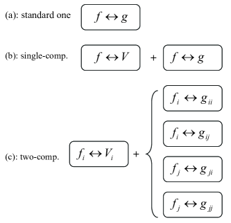
Figure 1: The unified physical picture for the balance between the different competitions for (a) the conventional NLS equation, (b) the single-component NLS equation and (c) the two-component NLS equation $i=1,2$ $(j=3-i)$ with harmonic external potential.

Here the expression of each $(1\rightleftharpoons 2)$ is obtained by interchanging the subscripts of 1 and 2 of the left term given in each row correspondingly in the right of the above equation, and $\lambda=\frac{\delta_{12}\delta_{21}}{\delta_{11}\delta_{22}}$. Four $\xi$ functions for the component $1$ read

$$\xi_{1,f_{1}\leftrightarrow g_{11}}(t)=2\varepsilon_{1}f_{1}(t)V_{1}(t)+\frac{d^{2}}{dt^{2}}\ln\frac{f_{1}(t)}{g_{11}(t)}$$

$$-\frac{d}{dt}\ln g_{11}(t)\frac{d}{dt}\ln\frac{f_{1}(t)}{g_{11}(t)},$$ (9)

$$\xi_{1,f_{1}\leftrightarrow g_{12}}(t)=2\varepsilon_{1}f_{1}(t)V_{1}(t)+\frac{d^{2}}{dt^{2}}\ln\frac{g_{22}(t)}{g_{21}(t)}\frac{f_{1}(t)}{g_{12}(t)}$$

$$-\frac{d}{dt}\ln\frac{g_{21}(t)}{g_{22}(t)}g_{12}(t)\frac{d}{dt}\ln\frac{g_{22}(t)}{g_{21}(t)}\frac{f_{1}(t)}{g_{12}(t)},$$ (10)

$$\xi_{1,f_{2}\leftrightarrow g_{21}}(t)=2\varepsilon_{1}f_{1}(t)V_{1}(t)+\frac{d^{2}}{dt^{2}}\ln\frac{f_{2}(t)}{g_{21}(t)}$$

$$-\frac{d}{dt}\ln\frac{f_{1}(t)}{f_{2}(t)}g_{21}(t)\frac{d}{dt}\ln\frac{f_{2}(t)}{g_{21}(t)},$$ (11)

$$\xi_{1,f_{2}\leftrightarrow g_{22}}(t)=2\varepsilon_{1}f_{1}(t)V_{1}(t)+\frac{d^{2}}{dt^{2}}\ln\frac{g_{12}(t)}{g_{11}(t)}\frac{f_{2}(t)}{g_{22}(t)}$$

$$-\frac{d}{dt}\ln\frac{f_{1}(t)}{f_{2}(t)}\frac{g_{11}(t)}{g_{12}(t)}g_{22}(t)\frac{d}{dt}\ln\frac{g_{12}(t)}{g_{11}(t)}\frac{f_{2}(t)}{g_{22}(t)}.$$ (12)

respectively. By the similar way, the $\xi$ functions of the component $2$ can be obtained by inter-exchanging the indices of $1$ and $2$ in the above four functions. These equations uncover the basic features for the integrability condition of the two-component NLS equation, as in the single-component case. That is the balance between the competition between the kinetic energy and the harmonic external potential and the competition between the dispersion and nonlinearity. In the two-component case, for each component there is one pair for the kinetic energy and the harmonic external potential, which competes with the different pairs of the dispersion and the nonlinearity, namely, $f_{1}\leftrightarrow g_{11}$, a contribution from the intra-component; $f_{1}\leftrightarrow g_{12}$, a contribution from the inter-component; $f_{2}\leftrightarrow g_{21}$ and $f_{2}\leftrightarrow g_{22}$, due to the existence of the component $2$ and relevant competitions between the dispersion and the nonlinearity in it. To clarify the above features, in Fig. 1 we show schematically this picture and make comparison with the cases in the single-component and the standard NLS equations. This result indicates that the integrability condition in these equations can be viewed as a unified picture, irrespective of the standard or nonautonomous systems.

IV Applications

The generalized integrability condition of Eq. (7) for the two-component nonautonomous NLS equation has not been reported in the literature. It can be used to investigate unique phenomenons in many practical two-component nonlinear systems. To further explore it, first we consider the symmetric case, such as $\varepsilon_{1}=\varepsilon_{2}=\varepsilon$, $f_{1}(t)=f_{2}(t)$, $g_{11}(t)=g_{22}(t)=g_{12}(t)=g_{21}(t)=g(t)$ and $V_{1}(t)=V_{2}(t)=V(t)$. Thus Eq. (7) reduces to

$$2\varepsilon f(t)V(t)+\frac{d^{2}}{dt^{2}}\ln\frac{f(t)}{g(t)}-\frac{d}{dt}\ln g(t)\frac{d}{dt}\ln\frac{f(t)}{g(t)}=0,$$ (13)

which is the same as that in the single-component case. Furthermore, if $\varepsilon=1/2$ and $f(t)=1$, Eq. (13) gives a constraint condition on the applied external potential

$$V(t)=\frac{1}{g(t)}\frac{d^{2}}{dt^{2}}g(t)-\frac{2}{g(t)^{2}}\left(\frac{d}{dt}g(t)\right)^{2}.$$ (14)

This expression is completely consistent with those reported in the literature Zhang2009 by using different methods. Under this condition, one may take a general transformation to obtain exact solution of the coupled NLS equation (4), as in the single-component case He2009

$$u_{i}(x,t)=U_{i}(X(x,t),T(t))\mbox{e}^{ia(x,t)+c(t)},$$ (15)

where $U_{i}(i=1,2)$ satisfy the standard coupled NLS equation

$$i\frac{\partial}{\partial T}U_{i}(X,T)+\varepsilon_{i}\frac{\partial^{2}}{\partial X^{2}}U_{i}(X,T)+\delta_{ii}|U_{i}(X,T)|^{2}U_{i}(X,T)$$

$$\hskip 85.35826pt+\delta_{ij}|U_{j}(X,T)|^{2}U_{i}(X,T)=0.$$ (16)

The explicit forms of $X(x,t),T(t),a(x,t)$ and $c(t)$ can be obtained analytically as follows $a(x,t)=\frac{1}{4\varepsilon f(t)}\left(\frac{d}{dt}\ln\frac{f(t)}{g(t}\right)x^{2}+C\frac{g(t)}{f(t)}x-\varepsilon C^{2}\int\frac{g^{2}(t)}{f(t)}dt$, $X(x,t)=\frac{g(t)}{f(t)}x-2\varepsilon C\int\frac{g^{2}(t)}{f(t)}dt$, $c(t)=\frac{1}{2}\ln\left(\frac{g(t)}{f(t)}\right)$, and $T(t)=\int\frac{g^{2}(t)}{f(t)}dt$, where $C$ is an arbitrary constant. Eq. (16) has a standard two-soliton solutions Adrian1997 , from which the corresponding nonautonomous two-soliton solutions of Eq. (4) can be explicitly obtained by Eq. (15). To understand the influence of Feshbach resonance on nonautonomous two-dark-bright soliton behavior under the integrability condition Eq. (13), we investigate the dynamics of these solitons with Feshbach management. These solitons can be realized in a two-component system such as different hyperfine spin states Myatt1997 . $g(t)$ is modulated periodically as $g(t)=1+\lambda\sin(\omega t)$, where $\lambda$ and $\omega$ are the relevant modulation parameters. The corresponding trap potential is tuned by Eq. (14). In Fig. 2 we show the nonautonomous two-dark-bright solitons dynamics obtained (c, d) and also compare them with the canonical ones (a, b). The result shows clearly that these solitons remain stable, as the conventional ones, but their shapes and speeds change with time. It is significant to guide experimental control over the dynamic behavior of the muti-solitons in binary BECs.

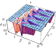
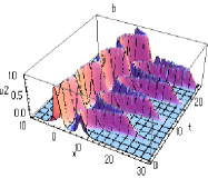
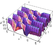
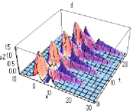
Figure 2: (Color online) The standard two dark-bright solitons (a, b) and the corresponding nonautonomous dark-bright solitons with the Feshbach management (c, d). The parameters used are $\lambda=0.5$ and $\omega=1$. The other parameters used are $a_{1}=1,$ $a_{2}=0.77,$ $b_{1}=b_{2}=0,$ $c=0$ and $\tau=1.$

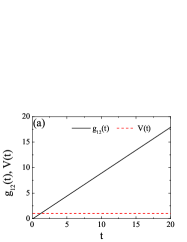
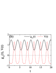
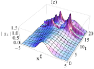
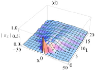
Figure 3: (Color online) Spatial separation of two components in the nonintegrable (a, c) case for $\lambda=1$ and the integrable (b, d) case for $\lambda=0.5$ and $\omega=2.$

Finally, we consider the phase separation phenomenon in binary BEC. For simplicity, we let $\delta_{11}=\delta_{22}=\delta_{12}=\delta_{21}=-1$, $f_{i}(t)=1$, $\varepsilon_{i}=1/2$, $g_{ii}(t)=1$ and $V_{i}(t)=V(t)$ ($i=1,2$). Thus Eq. (7) becomes

$$V(t)=\frac{1}{1+g_{12}(t)}\frac{d^{2}}{dt^{2}}g_{12}(t)-\frac{2}{(1+g_{12}(t))^{2}}\left(\frac{d}{dt}g_{12}(t)\right)^{2}.$$ (17)

Unfortunately, the explicit solution of Eq. (4) can not be obtained directly from that of Eq. (16) in this case, but it is enough to use the Gaussian wave packets to explore the spatial separation problem. They read Navarro2009

$$u_{1}(x,t)=A(t)e^{-\frac{\left(x-B(t)\right)^{2}}{2W(t)^{2}}}e^{i\left(C(t)+D(t)x+E(t)x^{2}\right)},$$

$$u_{2}(x,t)=A(t)e^{-\frac{\left(x+B(t)\right)^{2}}{2W(t)^{2}}}e^{i\left(C(t)-D(t)x+E(t)x^{2}\right)},$$ (18)

where $A(t),$ $B(t),$ $C(t),$ $D(t),$ $E(t)$ and $W(t)$ are the variational parameters and are determined by a set of ordinary differential equations given by Ref. Navarro2009 .

We solve this set of equations in two different cases. The first one is to increase intercomponent interaction linearly but fix the harmonic external potential as shown in Fig. 3(a). Initially the two components are mixed and keep miscible for some time. Subsequently the spatial separation happens. This is in agreement with the previous observation Navarro2009 . However, it is necessary to point out that this case is not integrable. In contrast, in the second case we consider the integrable constraint on the harmonic external potential given by Eq. (17). Here the intercomponent interaction assumed varies around 1 periodically, as shown in Fig. 3(b). In this case the applied external potential is modulated periodically following the intercomponent interaction. The two components in this case are found immiscible, even if the miscible condition $g_{12}(t)<1$ is satisfied frequently. This is a consequence of the change in the external potential, or rather the presence of the potential barrier ($V(t)<0$) in some time, which leads to the two-component separation shown in Fig. 3(d). The two different results provide possible ways to realize two-component spatial separations in binary BECs.

V Summary

By analyzing the integrability conditions of the nonautonomous NLS equations we found that the nature of the nonautonomous soliton is due to the balance between different competition features: the kinetic energy versus potential energy and the dispersion versus nonlinearity. This picture is consistent with the conventional one which originates from the balance between the dispersion and nonlinearity. On the other hand, the integrability conditions in two-component case is useful to guide experimental control over the dynamic of nonautonomous solitons and two-component separation in binary BECs.

VI Acknowledgements

The work is supported by the Program for NCET, NSF and the Fundamental Research Funds for the Central Universities of China. WML is supported by NSFC (No. 10934010) and the NKBRSFC (No. 2011CB921500).

References

- (1) N. J. Zabusky and M. D. Kruskal, Phys. Rev. Lett. 15, 240 (1965).
- (2) A. Hasegawa and Y. Kodama, Solitons in optical communications (Oxford University Press,Oxford, 1995).
- (3) H. A. Haus and W. S. Wong, Rev. Mod. Phys. 68, 423 (1996).
- (4) M. H. J. Anderson, J. R. Ensher, M. R. Matthews, and C. E. Wieman, Science 269, 198 (1995).
- (5) K. B. Davis, M.-O. Mewes, M. R. Andrews, N. J. van Druten, D. S. Durfee, D. M. Kurn, and W. Ketterle, Phys. Rev. Lett. 75, 3969 (1995).
- (6) S. Inouye et al., Nature (London) 392, 151 (1998); J. L. Roberts et al., Phys. Rev. Lett. 81, 5109 (1998).
- (7) P. G. Kevrekidis, G. Theocharis, D. J. Frantzeskakis, and B. A. Malomed, Phys. Rev. Lett. 90, 230401 (2003).
- (8) H.-H. Chen and C.-S. Liu, Phys. Rev. Lett. 37, 693 (1976).
- (9) F. Calogero and A. Degasperis, Lett. Nuovo Cimento Soc. Ital. Fis. 16, 425 (1976); 16, 434 (1976).
- (10) V. V. Konotop, Phys. Rev. E 47, 1423 (1993); V. V. Konotop, O. A. Chubykalo, and L. Vázquez, Phys. Rev. E 48, 563 (1993).
- (11) V. N. Serkin and A. Hasegawa, Phys. Rev. Lett. 85, 4502 (2000); IEEE J. Sel. Top. Quantum Electron. 8, 418 (2002).
- (12) V. I. Kruglov, A. C. Peacock, and J. D. Harvey, Phys. Rev. Lett. 90, 113902 (2003); ibid. 92, 199402(2004).
- (13) V. N. Serkin, A. Hasegawa, and T. L. Belyaeva, Phys. Rev. Lett. 92, 199401 (2004).
- (14) Z. X. Liang, Z. D. Zhang, and W. M. Liu, Phys. Rev. Lett. 94, 050402 (2005); Q. Y. Li, Z.-D Li, L. Li, G. S. Fu, Optics Communications, 283, 3361 (2010).
- (15) V. N. Serkin, A. Hasegawa, and T. L. Belyaeva, Phys. Rev. Lett. 98, 074102 (2007).
- (16) J. Belmonte-Beitia, V. M. Perez-Garcia, V. Vekslerchik, and V. V. Konotop, Phys. Rev. Lett. 100, 164102 (2008).
- (17) D. Zhao, H.-G. Luo, and Y.-H Cai, Phys. Lett. A 372, 5644 (2008); X.-G. He, D. Zhao, L. Li, and H.-G. Luo, Phys. Rev. E 79, 056610 (2009).
- (18) A. Kundu, Phys. Rev. E 79, 015601(R) (2009).
- (19) V. N. Serkin, A. Hasegawa, and T. L. Belyaeva, Phys. Rev. A 81, 023610 (2010).
- (20) J. Weiss, M. Tabor and G. Carnevale, J. Math. Phys. 24, 522 (1983).
- (21) U. A. Khawaja, J. Math. Phys. 51, 053506 (2010);
- (22) X.-F. Zhang, X.-H. Hu, X.-X. Liu, and W. M. Liu, Phys. Rev. A 79, 033630 (2009); S. Rajendran, P. Muruganandam and M. Lakshmanan. J. Phys. B: At. Mol. Opt. Phys. 42, 145307 (2009); V. R. Kumar, R. Radha, and M. Wadati, Phys. Lett. A 374, 3685 (2010).
- (23) A. P. Sheppard and Y. S. Kivshar, Phys. Rev. E 55, 4773 (1997).
- (24) C. J. Myatt, E. A. Burt, R. W. Ghrist, E. A. Cornell, and C. E. Wieman, Phys. Rev. Lett. 78, 586 (1997).
- (25) R. Navarro, R. Carretero-González, and P. G. Kevrekidis, Phys. Rev. A 80, 023613 (2009).