Optimal Deterministic Auctions with Correlated Priors

Christos Papadimitriou
UC Berkeley
christos@cs.berkeley.edu
Research (partially) supported by NSF grant CCF-0964033 and by a Google University Research Award.
         George Pierrakosfootnotemark:
UC Berkeley
georgios@cs.berkeley.edu
Abstract

We revisit the problem of designing the profit-maximizing single-item auction, solved by Myerson in his seminal paper for the case in which bidder valuations are independently distributed. We focus on general joint distributions, seeking the optimal deterministic incentive compatible auction. We give a geometric characterization of the optimal auction, resulting in a duality theorem and an efficient algorithm for finding the optimal deterministic auction in the two-bidder case and an NP-completeness result for three or more bidders.

1 Introduction

Myerson’s paper [21] on optimal auction design is remarkable in several ways. It is not the first important paper on auctions of course [30], but it pioneers the point of view of its title: auction design, that is, the exploration and evaluation of a large design space in a mindset that is very much one of computer science. It is elegant and methodologically original and powerful, completely resolving this important and difficult problem and providing insights, lemmata, and methodology that would be useful in related contexts for decades. Myerson considers the auction of an item to bidders with private valuations whose prior distributions are independent and known, and seeks incentive compatible mechanisms that maximize auctioneer revenue. His simple and elegant solution involves the virtual valuation, a quantity each bidder can compute from their private valuation and the valuation distribution through a mathematical maneuver called ironing.

Myerson leaves open the case in which the valuations are correlated; in subsequent work, Crémer and McLean [8, 7] consider correlated valuations and solve the problem for the case where auctions are only required to be interim individually rational. In fact, in this framework the uncorrelated case is a singularity in the sense that in most cases (when the correlation has “full rank” in a certain precise sense) full surplus can be extracted in expectation through appropriate offers of lotteries to the bidders. Despite the elegance of their result, the fact that bidders may be charged merely for participating in the auction–lottery (including losers) has been criticized as rendering the auction impractical [20], especially for settings where agents may easily cancel their participation after the auction is conducted. It is therefore of tantamount importance to consider the question of designing the optimal ex post individually rational auction for correlated valuations. This is the question we consider, and in a sense completely answer, in the current paper.

This past decade saw the advent and rise of Algorithmic Game Theory [24, 22], a research tradition which can be seen as a complexity-theoretic critique of Mathematical Economics, with Internet in the backdrop. This point of view has yielded a host of important results and new insights, for example related to the complexity of equilibria [6, 9], the trade-offs between complexity, approximation, and incentive-compatibility in social welfare-maximizing mechanism design [22, 25], and (in an extended sense that includes on-line algorithms as a part of complexity theory) the price of anarchy [19, 29, 28]. However, there has been little progress in looking at Bayesian auctions à-la Myerson from this point of view. Ronen [26] came up with a mechanism for the correlated case that achieves half of the optimum revenue, while Ronen and Saberi [27] showed that no “ascending auction” can do better than 7/8, and they conjectured that all relevant auctions are ascending (incidentally, we disprove this conjecture by showing that the optimal two-bidder auction may not be ascending). Missing from these two papers, however, is a concrete sense of the ways in which this is a difficult problem. We provide this here.

There were several follow-up papers  [4, 17, 10], examining the extent to which simple mechanisms can achieve good approximations of Myerson’s optimal mechanism, and motivated by Myerson’s astonishing result that the optimal mechanism for the regular i.i.d. setting is simply a second-price auction with reserve prices. For the most part, these are positive results yielding constant approximations by simple mechanisms in a variety of settings. Another line of work is prior-free mechanism design, where the goal is to design mechanisms that achieve profits comparable to that of some well-behaved benchmark [13]. This direction became especially interesting after Hartline and Roughgarden developed a framework in [16] that is grounded in Bayesian optimal mechanism design allowing one to design mechanisms that simultaneously approximate all Bayesian optimal mechanisms. The intermediate approach of having bidders’ valuations coming from a distribution that is nonetheless unknown to the auctioneer has also been considered [10]. Finally the important open problem of designing optimal multi-parameter mechanisms has been addressed for some distributions of preferences, such as additive valuations with budget constraints [2] and unit-demand settings [5] and connections of this problem to the algorithmic problem of optimal pricing have been made [4, 14]; economists have also made some attempts to extend Myerson’s results to multi-item auctions [1, 18].

In this paper we take a complexity-theoretic look at the general, correlated valuations case of Myerson’s single-item auctions. We point out that the optimal auction design problem can be reduced essentially to a maximum weighted independent set problem in a particular graph whose vertices are all possible tuples of valuations (an uncountable set, of course, in the continuous case). If the distribution is discrete, this is an ordinary graph-theoretic problem; no such combinatorial characterization had been known, and this had been the main difficulty in developing an algorithmic and complexity-theoretic understanding of the problem. For discrete distributions, this leads directly to an efficient algorithm in the case of two bidders, where the graph is bipartite, while in the case of three or more bidders NP-completeness (in fact, inapproximability) prevails. For continuous distributions, we prove a duality characterization through a Monge-Kantorovich-like problem [12], and from this a fully polynomial approximation scheme for two bidders when the distribution is continuous enough and accessible through an oracle — plus, as an aside, a 2/3 approximation for three bidders, improving the previously best known approximation of [26].

Our results rest on a geometric characterization of optimal deterministic auctions. An important element of our proof is the so-called marginal profit contribution function; it bears some similarities to Myerson’s virtual valuation function [21], the most important of them being that they both admit a marginal revenue interpretation in the spirit of [3]. However, despite their similarities and their somewhat common derivation, marginal profit contribution functions are different from Myerson’s virtual valuations in a number of ways: they only take positive values, they are not necessarily monotone and they do not admit a natural interpretation as valuations in some modified domain. One important ingredient of Myerson’s approach to the design of optimal auctions is an analytical maneuver he calls ironing; Myerson uses ironing to transform a potentially non-monotone allocation rule into a monotone one, without hurting revenue. Our approach circumvents ironing by restricting the space of mechanisms explored; we achieve that by imposing an additional technical condition which limits the design space into a subset of all mechanisms, but one which still contains all the optimal mechanisms.

The work most related to ours is that of Dobzinski, Fu and Kleinberg [11], who also study the problem of designing the optimal auction for the correlated setting. They obtain a collection of very interesting results, which however are quite complementary to ours: Based, among others, on insights from [26], they arrive at efficient algorithms for computing the optimal randomized mechanism that is truthful in expectation, and a constant factor approximation of the optimal deterministic auction for any number of bidders.

2 Preliminaries

Imagine n𝑛n bidders seeking an indivisible good offered in auction. We assume that each bidder has a private valuation visubscript𝑣𝑖v_{i} for the item and that bidders’ valuations are drawn from some joint distribution over [0,1]nsuperscript01𝑛[0,1]^{n} whose density function we denote by ϕ(𝐯)italic-ϕ𝐯\phi(\bf{v}). We consider both discrete and continuous ϕitalic-ϕ\phi. Discrete distributions are the source of the combinatorial insights underlying our approach, while continuous distributions provide continuity with the spirit and methodology of Myerson’s paper, another important source of inspiration. In the continuous case, we follow Myerson in making the analytically convenient assumption that ϕ(x)>0italic-ϕ𝑥0\phi(x)>0 for all x[0,1]n𝑥superscript01𝑛x\in[0,1]^{n}. This is hardly a loss of generality, since a small minimum value on every point can be achieved by changing ϕitalic-ϕ\phi very little. In stating an algorithm for the two-dimensional continuous case (Section 5), we shall also assume that ϕitalic-ϕ\phi is Lipschitz-continuous and accessible through an oracle (in such a way that, for example, it can be approximately integrated over nice regions).

In the discrete case, let Sup(ϕ)𝑆𝑢𝑝italic-ϕSup(\phi) denote the finite support of the joint discrete distribution ϕitalic-ϕ\phi. Then ϕitalic-ϕ\phi is presented as a finite set of |Sup(ϕ)|𝑆𝑢𝑝italic-ϕ|Sup(\phi)| (n+1)𝑛1(n+1)-tuples of the form (v1i,v2i,,vni,ϕi)superscriptsubscript𝑣1𝑖superscriptsubscript𝑣2𝑖superscriptsubscript𝑣𝑛𝑖superscriptitalic-ϕ𝑖(v_{1}^{i},v_{2}^{i},\ldots,v_{n}^{i},\phi^{i}), one for each point viSup(ϕ)superscript𝑣𝑖𝑆𝑢𝑝italic-ϕv^{i}\in Sup(\phi), where ϕisuperscriptitalic-ϕ𝑖\phi^{i} is the probability mass concentrated at the point (vi)superscript𝑣𝑖(v^{i}) of the support.

We are interested in designing auctions that maximize the auctioneer’s profit. Formally, an auction consists of an allocation rule denoted by xi(𝐯)subscript𝑥𝑖𝐯x_{i}(\bf{v}), the probability of bidder i𝑖i getting allocated the item, and a payment rule denoted by pi(𝐯)subscript𝑝𝑖𝐯p_{i}(\bf{v}) which is the price paid by bidder i𝑖i. In this paper we focus our attention on deterministic mechanisms so that xi(𝐯){0,1}subscript𝑥𝑖𝐯01x_{i}({\bf v})\in\{0,1\}. Our goal is to maximize the auctioneer’s expected profit i=1n𝔼[ϕ(𝐯)pi(𝐯)]superscriptsubscript𝑖1𝑛𝔼delimited-[]italic-ϕ𝐯subscript𝑝𝑖𝐯\sum_{i=1}^{n}\mathbb{E}\left[\phi({\bf v})p_{i}({\bf v})\right].

We want our auction to be ex-post incentive compatible (IC) and individually rational (IR), with no positive transfers (NPT). These notions are defined as follows:

  • IC:

    i,vi,vi,vi:vixi(vi,vi)pi(vi,vi)vixi(vi,vi)pi(vi,vi):for-all𝑖subscript𝑣𝑖subscriptsuperscript𝑣𝑖subscript𝑣𝑖subscript𝑣𝑖subscript𝑥𝑖subscript𝑣𝑖subscript𝑣𝑖subscript𝑝𝑖subscript𝑣𝑖subscript𝑣𝑖subscript𝑣𝑖subscript𝑥𝑖subscriptsuperscript𝑣𝑖subscript𝑣𝑖subscript𝑝𝑖subscriptsuperscript𝑣𝑖subscript𝑣𝑖\forall i,v_{i},v^{\prime}_{i},v_{-i}:v_{i}x_{i}(v_{i},v_{-i})-p_{i}(v_{i},v_{-i})\geq v_{i}x_{i}(v^{\prime}_{i},v_{-i})-p_{i}(v^{\prime}_{i},v_{-i})

  • IR:

    i,vi,vi:vixi(vi,vi)pi(vi,vi)0:for-all𝑖subscript𝑣𝑖subscript𝑣𝑖subscript𝑣𝑖subscript𝑥𝑖subscript𝑣𝑖subscript𝑣𝑖subscript𝑝𝑖subscript𝑣𝑖subscript𝑣𝑖0\forall i,v_{i},v_{-i}:v_{i}x_{i}(v_{i},v_{-i})-p_{i}(v_{i},v_{-i})\geq 0

  • NPT:

    i,vi,vi:pi(vi,vi)0:for-all𝑖subscript𝑣𝑖subscript𝑣𝑖subscript𝑝𝑖subscript𝑣𝑖subscript𝑣𝑖0\forall i,v_{i},v_{-i}:p_{i}(v_{i},v_{-i})\geq 0

We say that an allocation function xi(vi,vi)subscript𝑥𝑖subscript𝑣𝑖subscript𝑣𝑖x_{i}(v_{i},v_{-i}) is monotone if vivisubscript𝑣𝑖subscriptsuperscript𝑣𝑖v_{i}\geq v^{\prime}_{i} implies xi(vi,vi)xi(vi,vi)subscript𝑥𝑖subscript𝑣𝑖subscript𝑣𝑖subscript𝑥𝑖subscriptsuperscript𝑣𝑖subscript𝑣𝑖x_{i}(v_{i},v_{-i})\geq x_{i}(v^{\prime}_{i},v_{-i}) for all i,vi𝑖subscript𝑣𝑖i,v_{-i}. For the case of deterministic mechanisms that we are interested in monotonicity implies that xi(vi,vi)subscript𝑥𝑖subscript𝑣𝑖subscript𝑣𝑖x_{i}(v_{i},v_{-i}) is a step-function. The threshold value of such a step-function allocation rule is set to be the minimum winning valuation for every player given the valuations of the other bidders: ti(vi)=inf{vi[0,1]xi(vi,vi)=1}subscript𝑡𝑖subscript𝑣𝑖infimumconditional-setsubscript𝑣𝑖01subscript𝑥𝑖subscript𝑣𝑖subscript𝑣𝑖1t_{i}(v_{-i})=\inf\{v_{i}\in[0,1]\mid x_{i}(v_{i},v_{-i})=1\}.

The following theorem provides a characterization of mechanisms for the setting we are interested in; a proof can be found in [23].

Theorem 2.1.

A deterministic mechanism satisfies ICIC\mathrm{IC}, IRIR\mathrm{IR} and NPTNPT\mathrm{NPT} if and only if the following conditions hold.

  1. 1.

    xi(vi,vi)subscript𝑥𝑖subscript𝑣𝑖subscript𝑣𝑖x_{i}(v_{i},v_{-i}) is monotone.

  2. 2.

    For all i,vi,vi𝑖subscript𝑣𝑖subscript𝑣𝑖i,v_{i},v_{-i} we have

    pi(vi,vi)={ti(vi)if xi(vi,vi)=1;0if xi(vi,vi)=0.subscript𝑝𝑖subscript𝑣𝑖subscript𝑣𝑖casessubscript𝑡𝑖subscript𝑣𝑖if xi(vi,vi)=10if xi(vi,vi)=0p_{i}(v_{i},v_{-i})=\left\{\begin{array}[]{ll}t_{i}(v_{-i})&\mbox{if $x_{i}(v_{i},v_{-i})=1$};\\ 0&\mbox{if $x_{i}(v_{i},v_{-i})=0$}.\end{array}\right.

3 The Geometry of Optimal Auctions

Here we focus on the two-bidder case, and provide an alternative geometric interpretation of the mechanism design problem as a space partitioning problem. Our characterization holds for any number of bidders, with the appropriate generalizations and modifications; however we only address the multi-dimensional case in Section 6, where we will use our geometric characterization to establish the inapproximability of the problem for 3 or more bidders.

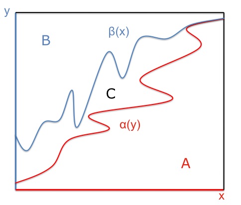
We start by noting that the allocation function can be described in terms of a partition of the unit square (the space of all possible valuation pairs) into three regions: In region A𝐴A bidder 1 gets the item, in region B𝐵B bidder 2 gets the item and in region C𝐶C neither gets the item. The shape of those regions is restricted by monotonicity as follows (see Figure 1): Region A𝐴A is rightward closed, meaning that (x,y)A𝑥𝑦𝐴(x,y)\in A and x>xsuperscript𝑥𝑥x^{\prime}>x implies (x,y)Asuperscript𝑥𝑦𝐴(x^{\prime},y)\in A, while region B𝐵B is, analogously, upward closed. These regions are captured by their boundaries: Region A𝐴A’s boundary is a function α:[0,1][0,1]:𝛼maps-to0101\alpha:[0,1]\mapsto[0,1] where for all y[0,1]𝑦01y\in[0,1] α(y)=inf{x:(x,y)A}𝛼𝑦infimumconditional-set𝑥𝑥𝑦𝐴\alpha(y)=\inf\{x:(x,y)\in A\}, and similarly for region B𝐵B and its boundary β(x)𝛽𝑥\beta(x).

Refer to caption
Figure 1: A pair of valid allocation rules.
Definition 3.1.

A valid allocation pair (α,β)𝛼𝛽(\alpha,\beta) is a pair of functions from [0,1]01[0,1] to itself satisfying the non-crossing property: for all points (x,y)[0,1]2𝑥𝑦superscript012(x,y)\in[0,1]^{2} we have yβ(x)xα(y)𝑦𝛽𝑥𝑥𝛼𝑦y\geq\beta(x)\Rightarrow x\leq\alpha(y).

Notice that it is not necessary for the functions to be monotone; the monotonicity property of the allocation is ensured through the fact that α𝛼\alpha and β𝛽\beta are proper functions and therefore regions A𝐴A and B𝐵B are rightward and upward closed respectively. The non-crossing property ensures that for any bid pair (x,y)𝑥𝑦(x,y) at most one bidder is allocated the item.

In our proof we will make extensive use of the following notion of marginal profit.

Definition 3.2.

Let f𝑓f (respectively, g𝑔g) be the marginal profit contribution of a bid pair (x,y)𝑥𝑦(x,y) for player 1 (resp. 2) defined as:

f(x,y)=x[maxxxxx1ϕ(t,y)𝑑t],g(x,y)=y[maxyyyy1ϕ(x,t)𝑑t]formulae-sequence𝑓𝑥𝑦𝑥delimited-[]subscriptsuperscript𝑥𝑥superscript𝑥superscriptsubscriptsuperscript𝑥1italic-ϕ𝑡𝑦differential-d𝑡𝑔𝑥𝑦𝑦delimited-[]subscriptsuperscript𝑦𝑦superscript𝑦superscriptsubscriptsuperscript𝑦1italic-ϕ𝑥𝑡differential-d𝑡f(x,y)=-\frac{\partial}{\partial x}\left[\max_{x^{\prime}\geq x}x^{\prime}\cdot\int_{x^{\prime}}^{1}\phi(t,y)\,dt\right],g(x,y)=-\frac{\partial}{\partial y}\left[\max_{y^{\prime}\geq y}y^{\prime}\cdot\int_{y^{\prime}}^{1}\phi(x,t)\,dt\right]

wherever the derivative is defined, and is extended to the full range by right continuity.

Intuitively, f(x,y)dxdy𝑓𝑥𝑦𝑑𝑥𝑑𝑦f(x,y)\,dx\,dy is the added expected profit obtained from including the infinitesimal area dxdy𝑑𝑥𝑑𝑦dx\,dy to A𝐴A, that is, deciding to give the item to the first bidder if the valuations are x,y𝑥𝑦x,y; in Remark 3.5 we further discuss the intuition behind these functions and their relation to Myerson’s virtual valuation functions.

Definition 3.3.

Call a valid allocation pair proper if it satisfies the following condition:

α(y)α(y)1ϕ(t,y)𝑑t=maxxα(y)xx1ϕ(t,y)𝑑t,for all yβ(x)β(x)1ϕ(x,t)𝑑t=maxyβ(x)yy1ϕ(x,t)𝑑t,for all x}\left.\begin{aligned} \alpha(y)\cdot\int_{\alpha(y)}^{1}\phi(t,y)\,dt=\max_{x^{\prime}\geq\alpha(y)}x^{\prime}\cdot\int_{x^{\prime}}^{1}\phi(t,y)\,dt,~{}~{}~{}\text{for all }y\\ \beta(x)\cdot\int_{\beta(x)}^{1}\phi(x,t)\,dt=\max_{y^{\prime}\geq\beta(x)}y^{\prime}\cdot\int_{y^{\prime}}^{1}\phi(x,t)\,dt,~{}~{}~{}\text{for all }x\end{aligned}\right\}\qquad (1)

Marginal profit contribution functions provide us with an alternative way to express the objective of expected profit.

Lemma 3.4.

Let (α,β)𝛼𝛽(\alpha,\beta) be a proper valid allocation pair. Then the expected profit of any auction with payments defined as in Theorem 2.1 is:

01α(y)1f(x,y)𝑑x𝑑y+01β(x)1g(x,y)𝑑y𝑑xsuperscriptsubscript01superscriptsubscript𝛼𝑦1𝑓𝑥𝑦differential-d𝑥differential-d𝑦superscriptsubscript01superscriptsubscript𝛽𝑥1𝑔𝑥𝑦differential-d𝑦differential-d𝑥\int_{0}^{1}\int_{\alpha(y)}^{1}f(x,y)\,dx\,dy+\int_{0}^{1}\int_{\beta(x)}^{1}g(x,y)\,dy\,dx
Proof.

Let p1(x,y),p2(x,y)subscript𝑝1𝑥𝑦subscript𝑝2𝑥𝑦p_{1}(x,y),p_{2}(x,y) be the payment functions induced by the allocation rule (α,β)𝛼𝛽(\alpha,\beta) according to Theorem 2.1. Then the expected profit of our auction is:

0101p1(x,y)ϕ(x,y)𝑑x𝑑y+0101p2(x,y)ϕ(x,y)𝑑x𝑑ysuperscriptsubscript01superscriptsubscript01subscript𝑝1𝑥𝑦italic-ϕ𝑥𝑦differential-d𝑥differential-d𝑦superscriptsubscript01superscriptsubscript01subscript𝑝2𝑥𝑦italic-ϕ𝑥𝑦differential-d𝑥differential-d𝑦\displaystyle\int_{0}^{1}\int_{0}^{1}p_{1}(x,y)\phi(x,y)\,dx\,dy+\int_{0}^{1}\int_{0}^{1}p_{2}(x,y)\phi(x,y)\,dx\,dy
=\displaystyle= 01[α(y)α(y)1ϕ(t,y)𝑑t]𝑑y+01[β(x)β(x)1ϕ(x,t)𝑑t]𝑑xsuperscriptsubscript01delimited-[]𝛼𝑦superscriptsubscript𝛼𝑦1italic-ϕ𝑡𝑦differential-d𝑡differential-d𝑦superscriptsubscript01delimited-[]𝛽𝑥superscriptsubscript𝛽𝑥1italic-ϕ𝑥𝑡differential-d𝑡differential-d𝑥\displaystyle\int_{0}^{1}\left[\alpha(y)\cdot\int_{\alpha(y)}^{1}\phi(t,y)\,dt\right]\,dy+\int_{0}^{1}\left[\beta(x)\cdot\int_{\beta(x)}^{1}\phi(x,t)\,dt\right]\,dx
=\displaystyle= 01[maxxα(y)xx1ϕ(t,y)𝑑t]𝑑y+01[maxyβ(x)yy1ϕ(x,t)𝑑t]𝑑xsuperscriptsubscript01delimited-[]subscriptsuperscript𝑥𝛼𝑦superscript𝑥superscriptsubscriptsuperscript𝑥1italic-ϕ𝑡𝑦differential-d𝑡differential-d𝑦superscriptsubscript01delimited-[]subscriptsuperscript𝑦𝛽𝑥superscript𝑦superscriptsubscriptsuperscript𝑦1italic-ϕ𝑥𝑡differential-d𝑡differential-d𝑥\displaystyle\int_{0}^{1}\left[\max_{x^{\prime}\geq\alpha(y)}x^{\prime}\cdot\int_{x^{\prime}}^{1}\phi(t,y)\,dt\right]\,dy+\int_{0}^{1}\left[\max_{y^{\prime}\geq\beta(x)}y^{\prime}\cdot\int_{y^{\prime}}^{1}\phi(x,t)\,dt\right]\,dx
=\displaystyle= 01α(y)1f(x,y)𝑑x𝑑y+01β(x)1g(x,y)𝑑y𝑑xsuperscriptsubscript01superscriptsubscript𝛼𝑦1𝑓𝑥𝑦differential-d𝑥differential-d𝑦superscriptsubscript01superscriptsubscript𝛽𝑥1𝑔𝑥𝑦differential-d𝑦differential-d𝑥\displaystyle\int_{0}^{1}\int_{\alpha(y)}^{1}f(x,y)\,dx\,dy+\int_{0}^{1}\int_{\beta(x)}^{1}g(x,y)\,dy\,dx

where in the first equality we used the characterization of truthful payments as every player’s critical value, in the second equality we made use of condition (1) and in the last equality we made use of the definition of marginal profit contribution functions. ∎

Remark 3.5.

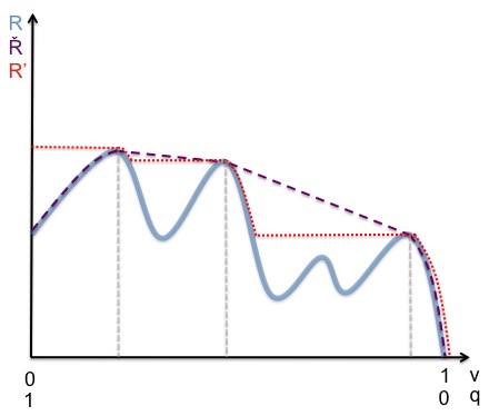
There is an intuitive connection between the marginal profit contribution and Myerson’s (ironed) virtual valuations [21]. As pointed out in the introduction, even though these functions are not identical, the goal in both cases is the same: to capture some notion of marginal revenue. Indeed the quantity xx1ϕ(t,y)𝑑t𝑥superscriptsubscript𝑥1italic-ϕ𝑡𝑦differential-d𝑡x\cdot\int_{x}^{1}\phi(t,y)\,dt corresponds to the expected profit of the auctioneer from an agent when she is offered a price of x𝑥x, keeping the value of the other player fixed at y𝑦y; equivalently one can write the expected revenue as a function R(q)𝑅𝑞R(q) of the probability of sale q=1x1ϕ(t,y)𝑑t𝑞1superscriptsubscript𝑥1italic-ϕ𝑡𝑦differential-d𝑡q=1-\int_{x}^{1}\phi(t,y)\,dt (for a thorough discussion of this maneuver the reader is referred to [15]). Myerson’s virtual valuations then correspond to the derivative of the function R(q)𝑅𝑞R(q), and ironing corresponds to taking the convex hull R^(q)^𝑅𝑞\hat{R}(q) of R(q)𝑅𝑞R(q) and then differentiating. The “ironing” in our case corresponds to the action of taking the derivative of R(q)=maxqqR(q)superscript𝑅𝑞subscriptsuperscript𝑞𝑞𝑅superscript𝑞R^{\prime}(q)=\max_{q^{\prime}\leq q}R(q^{\prime}) instead of R(q)𝑅𝑞R(q), which is intuitively the “skyline” one would see from q=0𝑞0q=0. In Figure 2 we show an example of a revenue curve R(q)𝑅𝑞R(q) and its corresponding R^(q)^𝑅𝑞\hat{R}(q) and R(q)superscript𝑅𝑞R^{\prime}(q) curves.

It has been already noted by Myerson [21] that the allocation rule will remain invariant across ironed regions: in his case this is a consequence of his proof technique involving ironing. In our case we explicitly demand that the allocation is invariant by imposing Condition 1. Since the invariance of the allocation rule across ironed regions follows from Myerson’s analysis as well, Condition 1 is indeed not a loss of generality in the sense that all optimal auctions satisfy it. We prove this formally next.

The next lemma establishes that without loss of generality we can restrict ourselves to proper allocation pairs. Let Profit(α,β,ϕ)𝑃𝑟𝑜𝑓𝑖𝑡𝛼𝛽italic-ϕProfit(\alpha,\beta,\phi) denote the profit of an auction with allocation curves (α,β)𝛼𝛽(\alpha,\beta), when the joint distribution of valuations is ϕitalic-ϕ\phi.

Lemma 3.6.

For any ϕitalic-ϕ\phi and for any valid allocation pair (α,β)𝛼𝛽(\alpha,\beta) there is a proper valid pair (α,β)superscript𝛼superscript𝛽(\alpha^{\prime},\beta^{\prime}) such that Profit(α,β,ϕ)Profit(α,β,ϕ)𝑃𝑟𝑜𝑓𝑖𝑡superscript𝛼superscript𝛽italic-ϕ𝑃𝑟𝑜𝑓𝑖𝑡𝛼𝛽italic-ϕProfit(\alpha^{\prime},\beta^{\prime},\phi)\geq Profit(\alpha,\beta,\phi)

Proof.

For the sake of contradiction suppose this is not true, i.e. Profit(α,β,ϕ)<Profit(α,β,ϕ)𝑃𝑟𝑜𝑓𝑖𝑡superscript𝛼superscript𝛽italic-ϕ𝑃𝑟𝑜𝑓𝑖𝑡𝛼𝛽italic-ϕProfit(\alpha^{\prime},\beta^{\prime},\phi)<Profit(\alpha,\beta,\phi) for any proper valid allocation pair (α,β)superscript𝛼superscript𝛽(\alpha^{\prime},\beta^{\prime}).

We start by defining the following sets of points:

𝒴={y[0,1]|α(y)α(y)1ϕ(t,y)𝑑tmaxxα(y)xx1ϕ(t,y)𝑑t}𝒴conditional-set𝑦01𝛼𝑦superscriptsubscript𝛼𝑦1italic-ϕ𝑡𝑦differential-d𝑡subscriptsuperscript𝑥𝛼𝑦superscript𝑥superscriptsubscriptsuperscript𝑥1italic-ϕ𝑡𝑦differential-d𝑡\mathcal{Y}=\left\{y\in[0,1]\ \middle|\ \alpha(y)\cdot\int_{\alpha(y)}^{1}\phi(t,y)\,dt\neq\max_{x^{\prime}\geq\alpha(y)}x^{\prime}\cdot\int_{x^{\prime}}^{1}\phi(t,y)\,dt\right\}
𝒳={x[0,1]|β(x)β(x)1ϕ(x,t)𝑑tmaxyβ(x)yy1ϕ(x,t)𝑑t}𝒳conditional-set𝑥01𝛽𝑥superscriptsubscript𝛽𝑥1italic-ϕ𝑥𝑡differential-d𝑡subscriptsuperscript𝑦𝛽𝑥superscript𝑦superscriptsubscriptsuperscript𝑦1italic-ϕ𝑥𝑡differential-d𝑡\mathcal{X}=\left\{x\in[0,1]\ \middle|\ \beta(x)\cdot\int_{\beta(x)}^{1}\phi(x,t)\,dt\neq\max_{y^{\prime}\geq\beta(x)}y^{\prime}\cdot\int_{y^{\prime}}^{1}\phi(x,t)\,dt\right\}

as the set of all coordinates y𝑦y (resp. x𝑥x) where condition (1) is violated by function α𝛼\alpha (resp. β𝛽\beta). Consider now the auction defined by the following allocation curves:

α(y)={α(y), if y𝒴;argmaxx{xx1ϕ(t,y)𝑑txα(y)}, if y𝒴.superscript𝛼𝑦cases𝛼𝑦, if y𝒴subscriptsuperscript𝑥conditionalsuperscript𝑥superscriptsubscriptsuperscript𝑥1italic-ϕ𝑡𝑦differential-d𝑡superscript𝑥𝛼𝑦, if y𝒴\alpha^{\prime}(y)=\left\{\begin{array}[]{ll}\alpha(y)&\mbox{, if $y\notin\mathcal{Y}$};\\ \arg\max_{x^{\prime}}\{x^{\prime}\int_{x^{\prime}}^{1}\phi(t,y)\,dt\mid x^{\prime}\geq\alpha(y)\}&\mbox{, if $y\in\mathcal{Y}$}.\end{array}\right.
β(x)={β(x), if x𝒳;argmaxy{yy1ϕ(x,t)𝑑tyβ(x)}, if x𝒳.superscript𝛽𝑥cases𝛽𝑥, if x𝒳subscriptsuperscript𝑦conditionalsuperscript𝑦superscriptsubscriptsuperscript𝑦1italic-ϕ𝑥𝑡differential-d𝑡superscript𝑦𝛽𝑥, if x𝒳\beta^{\prime}(x)=\left\{\begin{array}[]{ll}\beta(x)&\mbox{, if $x\notin\mathcal{X}$};\\ \arg\max_{y^{\prime}}\{y^{\prime}\int_{y^{\prime}}^{1}\phi(x,t)\,dt\mid y^{\prime}\geq\beta(x)\}&\mbox{, if $x\in\mathcal{X}$}.\end{array}\right.

where –in the case of ties– arg{}\arg\{\cdot\} returns the largest y𝑦y or x𝑥x respectively. By construction, the new pair (α,β)superscript𝛼superscript𝛽(\alpha^{\prime},\beta^{\prime}) satisfies condition (1). In what follows we claim that the resulting allocation pair (α,β)superscript𝛼superscript𝛽(\alpha^{\prime},\beta^{\prime}) is also valid and moreover it has greater revenue than (α,β)𝛼𝛽(\alpha,\beta), thus reaching a contradiction.

The monotonicity property of the allocation is satisfied since αsuperscript𝛼\alpha^{\prime} and βsuperscript𝛽\beta^{\prime} are proper functions of y𝑦y and x𝑥x respectively. The non-crossing property follows from the non-crossing property of α𝛼\alpha and β𝛽\beta and the fact that α(y)α(y)superscript𝛼𝑦𝛼𝑦\alpha^{\prime}(y)\geq\alpha(y) for all y[0,1]𝑦01y\in[0,1] and β(x)β(x)superscript𝛽𝑥𝛽𝑥\beta^{\prime}(x)\geq\beta(x) for all x[0,1]𝑥01x\in[0,1]. Finally, for the profit of the two auctions defined by the allocation curves (α,β)𝛼𝛽(\alpha,\beta) and (α,β)superscript𝛼superscript𝛽(\alpha^{\prime},\beta^{\prime}) we have:

Profit(α,β,ϕ)𝑃𝑟𝑜𝑓𝑖𝑡superscript𝛼superscript𝛽italic-ϕ\displaystyle Profit(\alpha^{\prime},\beta^{\prime},\phi)
=\displaystyle= 01[α(y)α(y)1ϕ(t,y)𝑑t]𝑑y+01[β(x)β(x)1ϕ(x,t)𝑑t]𝑑xsuperscriptsubscript01delimited-[]superscript𝛼𝑦superscriptsubscriptsuperscript𝛼𝑦1italic-ϕ𝑡𝑦differential-d𝑡differential-d𝑦superscriptsubscript01delimited-[]superscript𝛽𝑥superscriptsubscriptsuperscript𝛽𝑥1italic-ϕ𝑥𝑡differential-d𝑡differential-d𝑥\displaystyle\int_{0}^{1}\left[\alpha^{\prime}(y)\cdot\int_{\alpha^{\prime}(y)}^{1}\phi(t,y)\,dt\right]\,dy+\int_{0}^{1}\left[\beta^{\prime}(x)\cdot\int_{\beta^{\prime}(x)}^{1}\phi(x,t)\,dt\right]\,dx
\displaystyle\geq 01[α(y)α(y)1ϕ(t,y)𝑑t]𝑑y+01[β(x)β(x)1ϕ(x,t)𝑑t]𝑑xsuperscriptsubscript01delimited-[]𝛼𝑦superscriptsubscript𝛼𝑦1italic-ϕ𝑡𝑦differential-d𝑡differential-d𝑦superscriptsubscript01delimited-[]𝛽𝑥superscriptsubscript𝛽𝑥1italic-ϕ𝑥𝑡differential-d𝑡differential-d𝑥\displaystyle\int_{0}^{1}\left[\alpha(y)\cdot\int_{\alpha(y)}^{1}\phi(t,y)\,dt\right]\,dy+\int_{0}^{1}\left[\beta(x)\cdot\int_{\beta(x)}^{1}\phi(x,t)\,dt\right]\,dx
=\displaystyle= Profit(α,β,ϕ),𝑃𝑟𝑜𝑓𝑖𝑡𝛼𝛽italic-ϕ\displaystyle Profit(\alpha,\beta,\phi),

where the inequality follows from the definition of αsuperscript𝛼\alpha^{\prime} and βsuperscript𝛽\beta^{\prime}. The lemma now follows. ∎

Denote now by 𝒜𝒜\cal AB the set of all proper valid allocations (α,β)𝛼𝛽(\alpha,\beta). The problem of finding the optimal auction can now be restated as the following variational calculus-type problem:

Definition 3.7.

[Problem A]
sup(α,β)𝒜subscriptsupremum𝛼𝛽𝒜\displaystyle\sup_{(\alpha,\beta)\in{\cal AB}} {01α(y)1f(x,y)𝑑x𝑑y+01β(x)1g(x,y)𝑑y𝑑x}superscriptsubscript01superscriptsubscript𝛼𝑦1𝑓𝑥𝑦differential-d𝑥differential-d𝑦superscriptsubscript01superscriptsubscript𝛽𝑥1𝑔𝑥𝑦differential-d𝑦differential-d𝑥\displaystyle\left\{\int_{0}^{1}\int_{\alpha(y)}^{1}f(x,y)\,dx\,dy+\int_{0}^{1}\int_{\beta(x)}^{1}g(x,y)\,dy\,dx\right\}
Refer to caption
Figure 2: The revenue curves R𝑅R, R^^𝑅\hat{R} and Rsuperscript𝑅R^{\prime}.

4 Two Bidders: The Discrete Case

In this section we present an algorithm for computing the optimal mechanism when there are two bidders with a discrete joint distribution ϕitalic-ϕ\phi with support Sup(ϕ)=[N]×[N]𝑆𝑢𝑝italic-ϕdelimited-[]𝑁delimited-[]𝑁Sup(\phi)=[N]\times[N].

The marginal profit contribution functions defined in the previous section can be appropriately modified for the discrete setting in hand:

Definition 4.1.

The discrete analogues of the marginal profit contribution functions (Definition 3.2) for each player are defined as follows:

f(i,j)=max{iiiϕ(i,j)i>if(i,j),0}for player 1𝑓𝑖𝑗𝑖subscriptsuperscript𝑖𝑖italic-ϕsuperscript𝑖𝑗subscriptsuperscript𝑖𝑖𝑓superscript𝑖𝑗0for player 1f(i,j)=\max\left\{i\cdot\sum_{i^{\prime}\geq i}\phi(i^{\prime},j)-\sum_{i^{\prime}>i}f(i^{\prime},j),0\right\}~{}~{}\text{for player 1}
g(i,j)=max{jjjϕ(i,j)j>jg(i,j),0}for player 2𝑔𝑖𝑗𝑗subscriptsuperscript𝑗𝑗italic-ϕ𝑖superscript𝑗subscriptsuperscript𝑗𝑗𝑔𝑖superscript𝑗0for player 2g(i,j)=\max\left\{j\cdot\sum_{j^{\prime}\geq j}\phi(i,j^{\prime})-\sum_{j^{\prime}>j}g(i,j^{\prime}),0\right\}~{}~{}\text{for player 2}

As in the continuous case, we will represent the auction through a pair of functions (α,β)𝛼𝛽(\alpha,\beta):

Definition 4.2.

A valid allocation pair (α,β)𝛼𝛽(\alpha,\beta) for the discrete setting is a pair of functions from [N]delimited-[]𝑁[N] to itself satisfying the non-crossing property: for all points (i,j)[N]×[N]𝑖𝑗delimited-[]𝑁delimited-[]𝑁(i,j)\in[N]\times[N] we have jβ(i)i<α(j)𝑗𝛽𝑖𝑖𝛼𝑗j\geq\beta(i)\Rightarrow i<\alpha(j). Such a pair partitions the set Sup(ϕ)𝑆𝑢𝑝italic-ϕSup(\phi) into three sets A,B𝐴𝐵A,B, and C𝐶C, where A={(i,j)Sup(ϕ):iα(j)}𝐴conditional-set𝑖𝑗𝑆𝑢𝑝italic-ϕ𝑖𝛼𝑗A=\{(i,j)\in Sup(\phi):i\geq\alpha(j)\}, B={(i,j)Sup(ϕ):jβ(i)}𝐵conditional-set𝑖𝑗𝑆𝑢𝑝italic-ϕ𝑗𝛽𝑖B=\{(i,j)\in Sup(\phi):j\geq\beta(i)\}, and C=Sup(ϕ)AB𝐶𝑆𝑢𝑝italic-ϕ𝐴𝐵C=Sup(\phi)-A-B. We say that (α,β)𝛼𝛽(\alpha,\beta) induces the partition (A,B)𝐴𝐵(A,B), where C𝐶C is implicit.

Suppose that for a valid pair (α,β)𝛼𝛽(\alpha,\beta) representing an optimal auction and j[n]𝑗delimited-[]𝑛j\in[n], we have that f(α(j),j)=0𝑓𝛼𝑗𝑗0f(\alpha(j),j)=0. Then the auction represented by the same valid pair, except that α(j)𝛼𝑗\alpha(j) is increased by one, is also an optimal auction (since it entails the same set of positive marginal profit contributions). We can therefore consider, without loss of generality, only valid pairs with f(α(j),j),g(i,β(i))>0𝑓𝛼𝑗𝑗𝑔𝑖𝛽𝑖0f(\alpha(j),j),g(i,\beta(i))>0. We call such valid pairs proper. Finally, we define Π(ϕ)Πitalic-ϕ\Pi(\phi) to be the set of all partitions A,B𝐴𝐵A,B of Sup(ϕ)𝑆𝑢𝑝italic-ϕSup(\phi) induced by proper valid pairs.

Now, looking back at the formulation of the optimum-revenue auction problem in Problem A at the conclusion of the last section, it is immediate that obtaining the optimum-revenue auction in the discrete case is tantamount to solving a discrete optimization problem:

max(A,B)Π(ϕ)(i,j)Af(i,j)+(i,j)Bg(i,j).subscript𝐴𝐵Πitalic-ϕsubscript𝑖𝑗𝐴𝑓𝑖𝑗subscript𝑖𝑗𝐵𝑔𝑖𝑗\max_{(A,B)\in\Pi(\phi)}\sum_{(i,j)\in A}f(i,j)+\sum_{(i,j)\in B}g(i,j).

All that remains now is to provide a useful characterization of the set Π(ϕ)Πitalic-ϕ\Pi(\phi). To this end, notice first that any such pair of sets (A,B)𝐴𝐵(A,B) has the following two additional properties, the first one inherited from incentive compatibility, and the second one following from the fact that the allocation curves form a proper valid pair:

Definition 4.3.

We call a pair of disjoint subsets (A,B)𝐴𝐵(A,B) of Sup(ϕ)𝑆𝑢𝑝italic-ϕSup(\phi) monotone if the following holds:

  • If (i,j)A𝑖𝑗𝐴(i,j)\in A and (i,j)Sup(ϕ)superscript𝑖𝑗𝑆𝑢𝑝italic-ϕ(i^{\prime},j)\in Sup(\phi) with i>isuperscript𝑖𝑖i^{\prime}>i, then (i,j)Asuperscript𝑖𝑗𝐴(i^{\prime},j)\in A.

  • If (i,j)B𝑖𝑗𝐵(i,j)\in B and (i,j)Sup(ϕ)𝑖superscript𝑗𝑆𝑢𝑝italic-ϕ(i,j^{\prime})\in Sup(\phi) with j>jsuperscript𝑗𝑗j^{\prime}>j, then (i,j)B𝑖superscript𝑗𝐵(i,j^{\prime})\in B.

We call such a pair proper if

  • If (i,j)A𝑖𝑗𝐴(i,j)\in A and (i,j)Asuperscript𝑖𝑗𝐴(i^{\prime},j)\notin A for all i<isuperscript𝑖𝑖i^{\prime}<i, then f(i,j)>0𝑓𝑖𝑗0f(i,j)>0.

  • If (i,j)B𝑖𝑗𝐵(i,j)\in B and (i,j)B𝑖superscript𝑗𝐵(i,j^{\prime})\notin B for all j<jsuperscript𝑗𝑗j^{\prime}<j, then g(i,j)>0𝑔𝑖𝑗0g(i,j)>0. That is, in proper partitions, all lower boundary points of the regions A𝐴A and B𝐵B have positive marginal profit contributions (the intuition being that otherwise, either this is not an optimal auction in the case of a negative marginal contribution, or there is another optimal auction with this property in the case of a zero marginal contribution).

Let us define now a bipartite graph Gϕ=(U,W,E)superscript𝐺italic-ϕ𝑈𝑊𝐸G^{\phi}=(U,W,E):

  • U={ui,ji,j[N]}𝑈conditional-setsubscript𝑢𝑖𝑗𝑖𝑗delimited-[]𝑁U=\{u_{i,j}\mid i,j\in[N]\} and W={wi,ji,j[N]}𝑊conditional-setsubscript𝑤𝑖𝑗𝑖𝑗delimited-[]𝑁W=\{w_{i,j}\mid i,j\in[N]\};

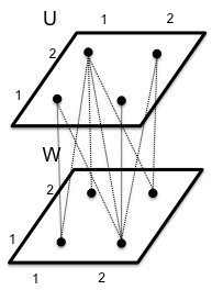
  • (ui,j,wi,j)Esubscript𝑢𝑖𝑗subscript𝑤superscript𝑖superscript𝑗𝐸(u_{i,j},w_{i^{\prime},j^{\prime}})\in E if and only if ii𝑖superscript𝑖i\leq i^{\prime} and jj𝑗superscript𝑗j\geq j^{\prime}. In other words, there is an edge between u𝑢u and w𝑤w if and only if, informally, (i,j)superscript𝑖superscript𝑗(i^{\prime},j^{\prime}) “lies to the southeast” of (i,j)𝑖𝑗(i,j) (see Figure 3); (Notice that, in our informal sense, a point “lies to the southeast” of all points to its north and to its west, including the point itself.)

  • The weight of any node ui,jsubscript𝑢𝑖𝑗u_{i,j} is f(i,j)𝑓𝑖𝑗f(i,j) and the weight of any node wi,jsubscript𝑤𝑖𝑗w_{i,j} is g(i,j)𝑔𝑖𝑗g(i,j).

Intuitively, the bipartite graph captures impossibilities in constructing the optimal auction: an edge (u,w)𝑢𝑤(u,w) signifies that it is not possible that both uA𝑢𝐴u\in A and wB𝑤𝐵w\in B (slightly abusing notation).

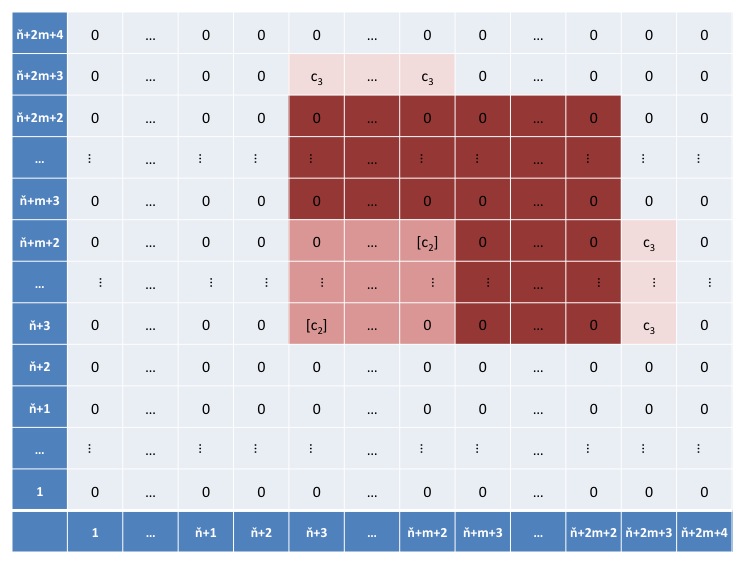
Refer to caption
Figure 3: The bipartite graph for 2 players with N=2𝑁2N=2.

We can now prove the sought combinatorial characterization of Π(ϕ)Πitalic-ϕ\Pi(\phi):

Lemma 4.4.

Let (A,B)𝐴𝐵(A,B) be a pair of disjoint subsets of Sup(ϕ)𝑆𝑢𝑝italic-ϕSup(\phi). Then (A,B)Π(ϕ)𝐴𝐵Πitalic-ϕ(A,B)\in\Pi(\phi) if and only if (A,B)𝐴𝐵(A,B) is monotone and proper, and {ui,j:(i,j)A}{wi,j:(i,j)B}conditional-setsubscript𝑢𝑖𝑗𝑖𝑗𝐴conditional-setsubscript𝑤𝑖𝑗𝑖𝑗𝐵\{u_{i,j}:(i,j)\in A\}\cup\{w_{i,j}:(i,j)\in B\} is an independent set of Gϕsuperscript𝐺italic-ϕG^{\phi}.

Proof.

(If.) Since {ui,j:(i,j)A}{wi,j:(i,j)B}conditional-setsubscript𝑢𝑖𝑗𝑖𝑗𝐴conditional-setsubscript𝑤𝑖𝑗𝑖𝑗𝐵\{u_{i,j}:(i,j)\in A\}\cup\{w_{i,j}:(i,j)\in B\} is an independent set of Gϕsuperscript𝐺italic-ϕG^{\phi} it follows that the sets A𝐴A and B𝐵B are disjoint. Now, since (A,B)𝐴𝐵(A,B) is a pair of monotone, proper and disjoint subsets of Sup(ϕ)𝑆𝑢𝑝italic-ϕSup(\phi) the following pair of functions (α(j),β(i))𝛼𝑗𝛽𝑖(\alpha(j),\beta(i)) is a proper valid pair, immediately implying that (A,B)Π(ϕ)𝐴𝐵Πitalic-ϕ(A,B)\in\Pi(\phi): α(j)=min{i(i,j)A}𝛼𝑗conditional𝑖𝑖𝑗𝐴\alpha(j)=\min\{i\mid(i,j)\in A\} and β(i)=min{j(i,j)B}𝛽𝑖conditional𝑗𝑖𝑗𝐵\beta(i)=\min\{j\mid(i,j)\in B\}.

(Only if.) If (A,B)Π(ϕ)𝐴𝐵Πitalic-ϕ(A,B)\in\Pi(\phi) then by the definition of Π(ϕ)Πitalic-ϕ\Pi(\phi) the sets (A,B)𝐴𝐵(A,B) have to be monotone and proper and they also need to form a partition, i.e. be disjoint. To show that {ui,j:(i,j)A}{wi,j:(i,j)B}conditional-setsubscript𝑢𝑖𝑗𝑖𝑗𝐴conditional-setsubscript𝑤𝑖𝑗𝑖𝑗𝐵\{u_{i,j}:(i,j)\in A\}\cup\{w_{i,j}:(i,j)\in B\} is an independent set of Gϕsuperscript𝐺italic-ϕG^{\phi} assume towards contradiction that there are nodes ui,jsubscript𝑢𝑖𝑗u_{i,j} and wi,jsubscript𝑤superscript𝑖superscript𝑗w_{i^{\prime},j^{\prime}} such that (i,j)A𝑖𝑗𝐴(i,j)\in A and (i,j)Bsuperscript𝑖superscript𝑗𝐵(i^{\prime},j^{\prime})\in B, with an edge between ui,jsubscript𝑢𝑖𝑗u_{i,j} and wi,jsubscript𝑤superscript𝑖superscript𝑗w_{i^{\prime},j^{\prime}}; from the construction of Gϕsuperscript𝐺italic-ϕG^{\phi}, it follows that ii𝑖superscript𝑖i\leq i^{\prime} and jj𝑗superscript𝑗j\geq j^{\prime}. Since A𝐴A and B𝐵B are both monotone, it follows that (i,j)ABsuperscript𝑖𝑗𝐴𝐵(i^{\prime},j)\in A\cap B, contradicting the disjointness of A𝐴A and B𝐵B. ∎

The next Lemma shows that the additional assumptions that (A,B)𝐴𝐵(A,B) is a proper and monotone pair of subsets are not necessary, if one restricts attention to the optimal solution (i.e. the solution of maximum weight).

Lemma 4.5.

Let (A,B)𝐴𝐵(A,B) be a pair of subsets of Sup(ϕ)𝑆𝑢𝑝italic-ϕSup(\phi) such that the set {ui,j:(i,j)A}{wi,j:(i,j)B}conditional-setsubscript𝑢𝑖𝑗𝑖𝑗𝐴conditional-setsubscript𝑤𝑖𝑗𝑖𝑗𝐵\{u_{i,j}:(i,j)\in A\}\cup\{w_{i,j}:(i,j)\in B\} is a maximum weight independent set of Gϕsuperscript𝐺italic-ϕG^{\phi}, of minimum cardinality among all independent sets of the same weight. Then (A,B)𝐴𝐵(A,B) is monotone and proper, i.e. (A,B)Π(ϕ)𝐴𝐵Πitalic-ϕ(A,B)\in\Pi(\phi).

Proof.

It suffices to show that the set (A,B)𝐴𝐵(A,B) is monotone and proper, and the lemma follows from Lemma 4.4. Indeed, the monotonicity of (A,B)𝐴𝐵(A,B) follows from the fact that the set {ui,j:(i,j)A}{wi,j:(i,j)B}conditional-setsubscript𝑢𝑖𝑗𝑖𝑗𝐴conditional-setsubscript𝑤𝑖𝑗𝑖𝑗𝐵\{u_{i,j}:(i,j)\in A\}\cup\{w_{i,j}:(i,j)\in B\} is a maximum weight independent set, and all weights are non-negative. Moreover, since the independent set has minimum cardinality among all independent sets of the same weight, it follows that it does not contain any node ui,jsubscript𝑢𝑖𝑗u_{i,j} of zero weight, i.e. corresponding to some valuation (i,j)𝑖𝑗(i,j) such that f(i,j)=0𝑓𝑖𝑗0f(i,j)=0, unless it also includes a node ui,jsubscript𝑢superscript𝑖𝑗u_{i^{\prime},j} corresponding to some valuation (i,j)superscript𝑖𝑗(i^{\prime},j) with f(i,j)>0𝑓superscript𝑖𝑗0f(i^{\prime},j)>0 for some i<isuperscript𝑖𝑖i^{\prime}<i (and analogously for wi,jsubscript𝑤𝑖𝑗w_{i,j}). Hence, by definition, (A,B)𝐴𝐵(A,B) is proper as well. ∎

Theorem 4.6.

Given a discrete joint valuation distribution ϕitalic-ϕ\phi for two bidders, the optimal ex-post IC and IR deterministic auction can be computed in time O(|Sup(ϕ)|3)𝑂superscript𝑆𝑢𝑝italic-ϕ3O(|Sup(\phi)|^{3}).

Proof.

It follows from Lemma 4.5 that computing the optimal auction for two bidders with a joint valuation distribution ϕitalic-ϕ\phi reduces to computing a maximum weight independent set on the induced bipartite graph Gϕsuperscript𝐺italic-ϕG^{\phi}. In particular the optimal allocation rule corresponds to a partition (A,B)𝐴𝐵(A,B) such that {ui,j:(i,j)A}{wi,j:(i,j)B}conditional-setsubscript𝑢𝑖𝑗𝑖𝑗𝐴conditional-setsubscript𝑤𝑖𝑗𝑖𝑗𝐵\{u_{i,j}:(i,j)\in A\}\cup\{w_{i,j}:(i,j)\in B\} is a maximum weight independent set of Gϕsuperscript𝐺italic-ϕG^{\phi}, with minimum cardinality among all independent sets of the same weight. Finding the maximum weight independent set by running a min-cost-flow algorithm yields the desired running time. ∎

5 Two Bidders: The General Case

In this section we return to the continuous two-bidder problem of Section 3. Our main result is an efficient algorithm that approximates the optimum solution of Problem A within an additive ϵitalic-ϵ\epsilon. Our main tool is a duality theorem, generalizing the duality between the maximum-weight independent set problem in a bipartite graph and a minimum-cost flow in an associate network. In particular, we show that the maximization Problem A defined in Section 3 is equivalent to a certain mass-moving minimization problem (reminiscent in some aspects of the classic Monge-Kantorovich [12] mass-transfer problem), namely the following:

Definition 5.1.

[Problem B]

infγsubscriptinfimum𝛾\displaystyle\inf_{\gamma} {01010y1x11γ(x1,y1,x2,y2)𝑑x2𝑑y2𝑑x1𝑑y1}superscriptsubscript01superscriptsubscript01superscriptsubscript0subscript𝑦1superscriptsubscriptsubscript𝑥11𝛾subscript𝑥1subscript𝑦1subscript𝑥2subscript𝑦2differential-dsubscript𝑥2differential-dsubscript𝑦2differential-dsubscript𝑥1differential-dsubscript𝑦1\displaystyle\left\{\int_{0}^{1}\int_{0}^{1}\int_{0}^{y_{1}}\int_{x_{1}}^{1}\gamma(x_{1},y_{1},x_{2},y_{2})\,dx_{2}\,dy_{2}\,dx_{1}\,dy_{1}\right\}
s.t.formulae-sequencest\displaystyle\mathrm{s.t.} 0y1x11γ(x1,y1,x2,y2)𝑑x2𝑑y2f(x1,y1),(x1,y1)[0,1]2formulae-sequencesuperscriptsubscript0subscript𝑦1superscriptsubscriptsubscript𝑥11𝛾subscript𝑥1subscript𝑦1subscript𝑥2subscript𝑦2differential-dsubscript𝑥2differential-dsubscript𝑦2𝑓subscript𝑥1subscript𝑦1for-allsubscript𝑥1subscript𝑦1superscript012\displaystyle\int_{0}^{y_{1}}\int_{x_{1}}^{1}\gamma(x_{1},y_{1},x_{2},y_{2})\,dx_{2}\,dy_{2}\geq f(x_{1},y_{1}),\,\forall(x_{1},y_{1})\in[0,1]^{2}
y210x2γ(x1,y1,x2,y2)𝑑x1𝑑y1g(x2,y2),(x2,y2)[0,1]2formulae-sequencesuperscriptsubscriptsubscript𝑦21superscriptsubscript0subscript𝑥2𝛾subscript𝑥1subscript𝑦1subscript𝑥2subscript𝑦2differential-dsubscript𝑥1differential-dsubscript𝑦1𝑔subscript𝑥2subscript𝑦2for-allsubscript𝑥2subscript𝑦2superscript012\displaystyle\int_{y_{2}}^{1}\int_{0}^{x_{2}}\gamma(x_{1},y_{1},x_{2},y_{2})\,dx_{1}\,dy_{1}\geq g(x_{2},y_{2}),\,\forall(x_{2},y_{2})\in[0,1]^{2}
γ(x1,y1,x2,y2)0,(x1,y1),(x2,y2)[0,1]2formulae-sequence𝛾subscript𝑥1subscript𝑦1subscript𝑥2subscript𝑦20for-allsubscript𝑥1subscript𝑦1subscript𝑥2subscript𝑦2superscript012\displaystyle\gamma(x_{1},y_{1},x_{2},y_{2})\geq 0,\,\forall(x_{1},y_{1}),(x_{2},y_{2})\in[0,1]^{2}

Let us denote by ΓΓ\Gamma the set of all functions γ:[0,1]4:𝛾maps-tosuperscript014\gamma:[0,1]^{4}\mapsto\Re satisfying the above constraints.

One intuitive interpretation of Problem B is this: We are given two landscapes in the unit square, captured by two functions f,g:[0,1]2:𝑓𝑔maps-tosuperscript012f,g:[0,1]^{2}\mapsto\Re. We are seeking a plan for transforming landscape f𝑓f to landscape g𝑔g, where the following operations are allowed:

  • take material away from any point (x,y)𝑥𝑦(x,y);

  • add material to any point (x,y)𝑥𝑦(x,y);

  • transfer material from any point to any other point in the southeast direction (if some material is not moved, we think of it as having moved in the southeast direction zero distance).

We want the plan in which the total amount of material moved (irrespective of distance moved, here is where this problem differs significantly from Monge-Kantorovich) is minimized. We next show that this problem coincides, at optimality, with the optimal auction:

Theorem 5.2.

[Duality Theorem]
For any joint density function ϕitalic-ϕ\phi on [0,1]2superscript012[0,1]^{2}:

sup(α,β)𝒜{01α(y)1f(x,y)𝑑x𝑑y+01β(x)1g(x,y)𝑑y𝑑x}subscriptsupremum𝛼𝛽𝒜superscriptsubscript01superscriptsubscript𝛼𝑦1𝑓𝑥𝑦differential-d𝑥differential-d𝑦superscriptsubscript01superscriptsubscript𝛽𝑥1𝑔𝑥𝑦differential-d𝑦differential-d𝑥\displaystyle\sup_{(\alpha,\beta)\in{\cal AB}}\left\{\int_{0}^{1}\int_{\alpha(y)}^{1}f(x,y)\,dx\,dy+\int_{0}^{1}\int_{\beta(x)}^{1}g(x,y)\,dy\,dx\right\}
=\displaystyle= infγΓ{01010y1x11γ(x1,y1,x2,y2)𝑑x2𝑑y2𝑑x1𝑑y1}subscriptinfimum𝛾Γsuperscriptsubscript01superscriptsubscript01superscriptsubscript0subscript𝑦1superscriptsubscriptsubscript𝑥11𝛾subscript𝑥1subscript𝑦1subscript𝑥2subscript𝑦2differential-dsubscript𝑥2differential-dsubscript𝑦2differential-dsubscript𝑥1differential-dsubscript𝑦1\displaystyle\inf_{\gamma\in\Gamma}\left\{\int_{0}^{1}\int_{0}^{1}\int_{0}^{y_{1}}\int_{x_{1}}^{1}\gamma(x_{1},y_{1},x_{2},y_{2})\,dx_{2}\,dy_{2}\,dx_{1}\,dy_{1}\right\}

5.1 Proof of the Duality Theorem

General Plan.

The proof of the theorem is by discretizing the unit square into domains of small size, proving a duality result for the discrete version, establishing upper bounds for the discretization error, and taking the limit for finer and finer discretization. In the course of the proof we will introduce a number of auxiliary problems.

Discretization.

We start by discretizing the continuous functions f𝑓f and g𝑔g defined on [0,1]×[0,1]0101[0,1]\times[0,1] by two discrete functions fdsubscript𝑓𝑑f_{d} and gdsubscript𝑔𝑑g_{d} defined on the [n]×[n]delimited-[]𝑛delimited-[]𝑛[n]\times[n] grid, where n𝑛n is an integer greater than one and [n]={0,1,…,n-1}; we denote 1n1𝑛1\over n by ϵitalic-ϵ\epsilon. We subdivide the [0,1]×[0,1]0101[0,1]\times[0,1] square into ϵ×ϵitalic-ϵitalic-ϵ\epsilon\times\epsilon little squares; we are mapping a little square with southwest coordinate (x,y)𝑥𝑦(x,y) to the grid point n(x,y)𝑛𝑥𝑦n\cdot(x,y). The discrete functions are now obtained by assigning to each point in the grid the aggregate mass of its corresponding square on the plane.

fd(i,j)=ϵiϵ(i+1)ϵjϵ(j+1)f(x,y)𝑑y𝑑x, for i,j=0,,n1formulae-sequencesubscript𝑓𝑑𝑖𝑗superscriptsubscriptitalic-ϵ𝑖italic-ϵ𝑖1superscriptsubscriptitalic-ϵ𝑗italic-ϵ𝑗1𝑓𝑥𝑦differential-d𝑦differential-d𝑥 for 𝑖𝑗0𝑛1f_{d}(i,j)=\int_{\epsilon i}^{\epsilon(i+1)}\int_{\epsilon j}^{\epsilon(j+1)}f(x,y)\,dy\,dx,\,\text{ for }i,j=0,\ldots,n-1

and

gd(i,j)=ϵiϵ(i+1)ϵjϵ(j+1)g(x,y)𝑑y𝑑x for i,j=0,,n1.formulae-sequencesubscript𝑔𝑑𝑖𝑗superscriptsubscriptitalic-ϵ𝑖italic-ϵ𝑖1superscriptsubscriptitalic-ϵ𝑗italic-ϵ𝑗1𝑔𝑥𝑦differential-d𝑦differential-d𝑥 for 𝑖𝑗0𝑛1g_{d}(i,j)=\int_{\epsilon i}^{\epsilon(i+1)}\int_{\epsilon j}^{\epsilon(j+1)}g(x,y)\,dy\,dx\,\text{ for }i,j=0,\ldots,n-1.
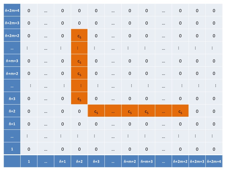
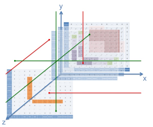
Refer to caption
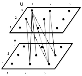
Figure 4: The graph consisting of two grids, one for each player, for n=3𝑛3n=3.

The Graph.

We next create a weighted bipartite graph G=(U,V,E)𝐺𝑈𝑉𝐸G=(U,V,E) as follows: U=V=[n]×[n]𝑈𝑉delimited-[]𝑛delimited-[]𝑛U=V=[n]\times[n]. We use u(i,j)𝑢𝑖𝑗u(i,j) and v(i,j)𝑣𝑖𝑗v(i,j) to denote the vertices of U𝑈U and V𝑉V respectively, and sometimes use the shorthand u𝑢u and v𝑣v to refer to nodes of each grid respectively. Vertex u(i,j)𝑢𝑖𝑗u(i,j) of U𝑈U has a weight equal to wu=fd(i,j)subscript𝑤𝑢subscript𝑓𝑑𝑖𝑗w_{u}=f_{d}(i,j), and similarly vertex v(i,j)𝑣superscript𝑖superscript𝑗v(i^{\prime},j^{\prime}) of V𝑉V has a weight wv=gd(i,j)subscript𝑤𝑣subscript𝑔𝑑superscript𝑖superscript𝑗w_{v}=g_{d}(i^{\prime},j^{\prime}). A pair (u(i,j),v(i,j))𝑢𝑖𝑗𝑣superscript𝑖superscript𝑗(u(i,j),v(i^{\prime},j^{\prime})) is in E𝐸E if and only if i<i𝑖superscript𝑖i<i^{\prime} and j>j𝑗superscript𝑗j>j^{\prime}, that is, if grid point v𝑣v is in the (strictly) Southeast direction from grid point u𝑢u (see Figure 4 for an example with n=3𝑛3n=3).

Consider now the following problem, familiar from the previous section:

Definition 5.3.

[Problem C: Maximum Weight Independent Set]
Given the weighted bipartite graph G=(U,V,E)𝐺𝑈𝑉𝐸G=(U,V,E) above,

max{xu{0,1},xv{0,1}}subscriptformulae-sequencesubscript𝑥𝑢01subscript𝑥𝑣01\displaystyle\max_{\{x_{u}\in\{0,1\},x_{v}\in\{0,1\}\}} uU,vVxuwu+xvwvsubscriptformulae-sequence𝑢𝑈𝑣𝑉subscript𝑥𝑢subscript𝑤𝑢subscript𝑥𝑣subscript𝑤𝑣\displaystyle\sum_{u\in U,v\in V}x_{u}w_{u}+x_{v}w_{v}
s.t.formulae-sequencest\displaystyle\mathrm{s.t.} xu+xv1,(u,v)Eformulae-sequencesubscript𝑥𝑢subscript𝑥𝑣1for-all𝑢𝑣𝐸\displaystyle x_{u}+x_{v}\leq 1,\,\forall(u,v)\in E

The dual of the above problem is the following:

Definition 5.4.

[Problem D: Minimum Cost Transshipment]
Given the weighted bipartite graph G=(U,V,E)𝐺𝑈𝑉𝐸G=(U,V,E) above,

min{yuv}subscriptsubscript𝑦𝑢𝑣\displaystyle\min_{\{y_{uv}\in\Re\}} (u,v)Eyuvsubscript𝑢𝑣𝐸subscript𝑦𝑢𝑣\displaystyle\sum_{(u,v)\in E}y_{uv}
s.t.formulae-sequencest\displaystyle\mathrm{s.t.} v:(u,v)Eyuvwu,uUformulae-sequencesubscript:𝑣𝑢𝑣𝐸subscript𝑦𝑢𝑣subscript𝑤𝑢for-all𝑢𝑈\displaystyle\sum_{v:(u,v)\in E}y_{uv}\geq w_{u},\,\forall u\in U
u:(u,v)Eyuvwv,vVformulae-sequencesubscript:𝑢𝑢𝑣𝐸subscript𝑦𝑢𝑣subscript𝑤𝑣for-all𝑣𝑉\displaystyle\sum_{u:(u,v)\in E}y_{uv}\geq w_{v},\,\forall v\in V
yuv0,(u,v)Eformulae-sequencesubscript𝑦𝑢𝑣0for-all𝑢𝑣𝐸\displaystyle y_{uv}\geq 0,\,\forall(u,v)\in E

The Inequalities.

The crux of the proof is a sequence of results relating the various solutions and optimum solutions of these four problems. In what follows we use SOL()𝑆𝑂𝐿SOL(\cdot) to denote the cost of any feasible solution of a problem among (A), (B), (C), and (D) defined above, and OPT()𝑂𝑃𝑇OPT(\cdot) to denote the cost of the optimum solution of a problem (sometimes SOL𝑆𝑂𝐿SOL and OPT𝑂𝑃𝑇OPT also denotes the actual solutions). The first such inequality establishes a form of weak duality between Problems A𝐴A and B𝐵B, while the next two show that the discretization error is small.

Lemma 5.5.

For any feasible solutions of A𝐴A and B𝐵B we have: SOL(A)SOL(B)𝑆𝑂𝐿𝐴𝑆𝑂𝐿𝐵SOL(A)\leq SOL(B).

Proof.
SOL(A)𝑆𝑂𝐿𝐴\displaystyle SOL(A)
=\displaystyle= 01α(y1)1f(x1,y1)𝑑x1𝑑y1+01β(x2)1g(x2,y2)𝑑y2𝑑x2superscriptsubscript01superscriptsubscript𝛼subscript𝑦11𝑓subscript𝑥1subscript𝑦1differential-dsubscript𝑥1differential-dsubscript𝑦1superscriptsubscript01superscriptsubscript𝛽subscript𝑥21𝑔subscript𝑥2subscript𝑦2differential-dsubscript𝑦2differential-dsubscript𝑥2\displaystyle\int_{0}^{1}\int_{\alpha(y_{1})}^{1}f(x_{1},y_{1})\,dx_{1}\,dy_{1}+\int_{0}^{1}\int_{\beta(x_{2})}^{1}g(x_{2},y_{2})\,dy_{2}\,dx_{2}
\displaystyle\leq 01α(y1)10y1x11γ(x1,y1,x2,y2)𝑑x2𝑑y2𝑑x1𝑑y1+01β(x2)1y210x2γ(x1,y1,x2,y2)𝑑x1𝑑y1𝑑y2𝑑x2superscriptsubscript01superscriptsubscript𝛼subscript𝑦11superscriptsubscript0subscript𝑦1superscriptsubscriptsubscript𝑥11𝛾subscript𝑥1subscript𝑦1subscript𝑥2subscript𝑦2differential-dsubscript𝑥2differential-dsubscript𝑦2differential-dsubscript𝑥1differential-dsubscript𝑦1superscriptsubscript01superscriptsubscript𝛽subscript𝑥21superscriptsubscriptsubscript𝑦21superscriptsubscript0subscript𝑥2𝛾subscript𝑥1subscript𝑦1subscript𝑥2subscript𝑦2differential-dsubscript𝑥1differential-dsubscript𝑦1differential-dsubscript𝑦2differential-dsubscript𝑥2\displaystyle\int_{0}^{1}\int_{\alpha(y_{1})}^{1}\int_{0}^{y_{1}}\int_{x_{1}}^{1}\gamma(x_{1},y_{1},x_{2},y_{2})\,dx_{2}\,dy_{2}\,dx_{1}\,dy_{1}+\int_{0}^{1}\int_{\beta(x_{2})}^{1}\int_{y_{2}}^{1}\int_{0}^{x_{2}}\gamma(x_{1},y_{1},x_{2},y_{2})\,dx_{1}\,dy_{1}\,dy_{2}\,dx_{2}

where we used the inequality constraints of Problem B to upper bound the values of f(x,y)𝑓𝑥𝑦f(x,y) and g(x,y)𝑔𝑥𝑦g(x,y). We next notice that:

01β(x2)1y210x2γ(x1,y1,x2,y2)𝑑x1𝑑y1𝑑y2𝑑x2010α(y1)0y1x11γ(x1,y1,x2,y2)𝑑x2𝑑y2𝑑x1𝑑y1superscriptsubscript01superscriptsubscript𝛽subscript𝑥21superscriptsubscriptsubscript𝑦21superscriptsubscript0subscript𝑥2𝛾subscript𝑥1subscript𝑦1subscript𝑥2subscript𝑦2differential-dsubscript𝑥1differential-dsubscript𝑦1differential-dsubscript𝑦2differential-dsubscript𝑥2superscriptsubscript01superscriptsubscript0𝛼subscript𝑦1superscriptsubscript0subscript𝑦1superscriptsubscriptsubscript𝑥11𝛾subscript𝑥1subscript𝑦1subscript𝑥2subscript𝑦2differential-dsubscript𝑥2differential-dsubscript𝑦2differential-dsubscript𝑥1differential-dsubscript𝑦1\int_{0}^{1}\int_{\beta(x_{2})}^{1}\int_{y_{2}}^{1}\int_{0}^{x_{2}}\gamma(x_{1},y_{1},x_{2},y_{2})\,dx_{1}\,dy_{1}\,dy_{2}\,dx_{2}\leq\int_{0}^{1}\int_{0}^{\alpha(y_{1})}\int_{0}^{y_{1}}\int_{x_{1}}^{1}\gamma(x_{1},y_{1},x_{2},y_{2})\,dx_{2}\,dy_{2}\,dx_{1}\,dy_{1}

This inequality follows from the non-negativity of γ𝛾\gamma and the fact that the (x1,y1,x2,y2)subscript𝑥1subscript𝑦1subscript𝑥2subscript𝑦2(x_{1},y_{1},x_{2},y_{2}) included in the integral of the LHS are the following set:

{(x1,y1,x2,y2)[0,1]4y2β(x2),x1x2,y1y2}conditional-setsubscript𝑥1subscript𝑦1subscript𝑥2subscript𝑦2superscript014formulae-sequencesubscript𝑦2𝛽subscript𝑥2formulae-sequencesubscript𝑥1subscript𝑥2subscript𝑦1subscript𝑦2\displaystyle\{(x_{1},y_{1},x_{2},y_{2})\in[0,1]^{4}\mid y_{2}\geq\beta(x_{2}),\ x_{1}\leq x_{2},\ y_{1}\geq y_{2}\}
=\displaystyle= {(x1,y1,x2,y2)[0,1]4y2β(x2),x1x2,y1y2,x1α(y1)}conditional-setsubscript𝑥1subscript𝑦1subscript𝑥2subscript𝑦2superscript014formulae-sequencesubscript𝑦2𝛽subscript𝑥2formulae-sequencesubscript𝑥1subscript𝑥2formulae-sequencesubscript𝑦1subscript𝑦2subscript𝑥1𝛼subscript𝑦1\displaystyle\{(x_{1},y_{1},x_{2},y_{2})\in[0,1]^{4}\mid y_{2}\geq\beta(x_{2}),\ x_{1}\leq x_{2},\ y_{1}\geq y_{2},\ x_{1}\leq\alpha(y_{1})\}
\displaystyle\subseteq {(x1,y1,x2,y2)[0,1]4x2α(y2),x1x2,y1y2,x1α(y1)}conditional-setsubscript𝑥1subscript𝑦1subscript𝑥2subscript𝑦2superscript014formulae-sequencesubscript𝑥2𝛼subscript𝑦2formulae-sequencesubscript𝑥1subscript𝑥2formulae-sequencesubscript𝑦1subscript𝑦2subscript𝑥1𝛼subscript𝑦1\displaystyle\{(x_{1},y_{1},x_{2},y_{2})\in[0,1]^{4}\mid x_{2}\leq\alpha(y_{2}),\ x_{1}\leq x_{2},\ y_{1}\geq y_{2},\ x_{1}\leq\alpha(y_{1})\}
\displaystyle\subseteq {(x1,y1,x2,y2)[0,1]4x1x2,y1y2,x1α(y1)}conditional-setsubscript𝑥1subscript𝑦1subscript𝑥2subscript𝑦2superscript014formulae-sequencesubscript𝑥1subscript𝑥2formulae-sequencesubscript𝑦1subscript𝑦2subscript𝑥1𝛼subscript𝑦1\displaystyle\{(x_{1},y_{1},x_{2},y_{2})\in[0,1]^{4}\mid x_{1}\leq x_{2},\ y_{1}\geq y_{2},\ x_{1}\leq\alpha(y_{1})\}

which is exactly the set of (x1,y1,x2,y2)subscript𝑥1subscript𝑦1subscript𝑥2subscript𝑦2(x_{1},y_{1},x_{2},y_{2}) included in the integral of the RHS. The first equality above follows from the fact that the inequality x1α(y1)subscript𝑥1𝛼subscript𝑦1x_{1}\leq\alpha(y_{1}) follows from the inequalities {y2β(x2),x1x2,y1y2}formulae-sequencesubscript𝑦2𝛽subscript𝑥2formulae-sequencesubscript𝑥1subscript𝑥2subscript𝑦1subscript𝑦2\{y_{2}\geq\beta(x_{2}),\ x_{1}\leq x_{2},\ y_{1}\geq y_{2}\}, because we have y1β(x2)subscript𝑦1𝛽subscript𝑥2y_{1}\geq\beta(x_{2}) so the non-crossing property implies that x2α(y1)subscript𝑥2𝛼subscript𝑦1x_{2}\leq\alpha(y_{1}) and therefore x1α(y1)subscript𝑥1𝛼subscript𝑦1x_{1}\leq\alpha(y_{1}). The first set inclusion follows from the fact that y2β(x2)x2α(y2)subscript𝑦2𝛽subscript𝑥2subscript𝑥2𝛼subscript𝑦2y_{2}\geq\beta(x_{2})\Rightarrow x_{2}\leq\alpha(y_{2}) from the non-crossing property, while the last inclusion is trivial.

We have therefore concluded that the cost of any feasible solution of A𝐴A is upper bounded by:

01α(y1)10y1x11γ(x1,y1,x2,y2)𝑑x2𝑑y2𝑑x1𝑑y1+010α(y1)0y1x11γ(x1,y1,x2,y2)𝑑x2𝑑y2𝑑x1𝑑y1superscriptsubscript01superscriptsubscript𝛼subscript𝑦11superscriptsubscript0subscript𝑦1superscriptsubscriptsubscript𝑥11𝛾subscript𝑥1subscript𝑦1subscript𝑥2subscript𝑦2differential-dsubscript𝑥2differential-dsubscript𝑦2differential-dsubscript𝑥1differential-dsubscript𝑦1superscriptsubscript01superscriptsubscript0𝛼subscript𝑦1superscriptsubscript0subscript𝑦1superscriptsubscriptsubscript𝑥11𝛾subscript𝑥1subscript𝑦1subscript𝑥2subscript𝑦2differential-dsubscript𝑥2differential-dsubscript𝑦2differential-dsubscript𝑥1differential-dsubscript𝑦1\displaystyle\int_{0}^{1}\int_{\alpha(y_{1})}^{1}\int_{0}^{y_{1}}\int_{x_{1}}^{1}\gamma(x_{1},y_{1},x_{2},y_{2})\,dx_{2}\,dy_{2}\,dx_{1}\,dy_{1}+\int_{0}^{1}\int_{0}^{\alpha(y_{1})}\int_{0}^{y_{1}}\int_{x_{1}}^{1}\gamma(x_{1},y_{1},x_{2},y_{2})\,dx_{2}\,dy_{2}\,dx_{1}\,dy_{1}
=\displaystyle= 01010y1x11γ(x1,y1,x2,y2)𝑑x2𝑑y2𝑑x1𝑑y1superscriptsubscript01superscriptsubscript01superscriptsubscript0subscript𝑦1superscriptsubscriptsubscript𝑥11𝛾subscript𝑥1subscript𝑦1subscript𝑥2subscript𝑦2differential-dsubscript𝑥2differential-dsubscript𝑦2differential-dsubscript𝑥1differential-dsubscript𝑦1\displaystyle\int_{0}^{1}\int_{0}^{1}\int_{0}^{y_{1}}\int_{x_{1}}^{1}\gamma(x_{1},y_{1},x_{2},y_{2})\,dx_{2}\,dy_{2}\,dx_{1}\,dy_{1}
=\displaystyle= SOL(B)𝑆𝑂𝐿𝐵\displaystyle SOL(B)

Lemma 5.6.

For the optimal solutions of A𝐴A and C𝐶C we have: OPT(A)OPT(C)ϵ𝑂𝑃𝑇𝐴𝑂𝑃𝑇𝐶italic-ϵOPT(A)\geq OPT(C)-\epsilon.

Proof.

Consider the optimal solution of Problem C𝐶C; we will use it to come up with a feasible solution for Problem A𝐴A such that SOL(A)OPT(C)ϵ𝑆𝑂𝐿𝐴𝑂𝑃𝑇𝐶italic-ϵSOL(A)\geq OPT(C)-\epsilon. We start with the following solution: we allocate the item to player 1 for all valuations (x,y)𝑥𝑦(x,y) such that xu(xϵ,yϵ)=1subscript𝑥𝑢𝑥italic-ϵ𝑦italic-ϵ1x_{u(\left\lfloor\frac{x}{\epsilon}\right\rfloor,\left\lfloor\frac{y}{\epsilon}\right\rfloor)}=1; we allocate to player 2 for all valuations (x,y)𝑥𝑦(x,y) such that xv(xϵ,yϵ)=1subscript𝑥𝑣𝑥italic-ϵ𝑦italic-ϵ1x_{v(\left\lfloor\frac{x}{\epsilon}\right\rfloor,\left\lfloor\frac{y}{\epsilon}\right\rfloor)}=1, and xu(xϵ,yϵ)=0subscript𝑥𝑢𝑥italic-ϵ𝑦italic-ϵ0x_{u(\left\lfloor\frac{x}{\epsilon}\right\rfloor,\left\lfloor\frac{y}{\epsilon}\right\rfloor)}=0; and finally, we allocate to nobody for all valuations (x,y)𝑥𝑦(x,y) such that xu(xϵ,yϵ)=0subscript𝑥𝑢𝑥italic-ϵ𝑦italic-ϵ0x_{u(\left\lfloor\frac{x}{\epsilon}\right\rfloor,\left\lfloor\frac{y}{\epsilon}\right\rfloor)}=0 and xv(xϵ,yϵ)=0subscript𝑥𝑣𝑥italic-ϵ𝑦italic-ϵ0x_{v(\left\lfloor\frac{x}{\epsilon}\right\rfloor,\left\lfloor\frac{y}{\epsilon}\right\rfloor)}=0.

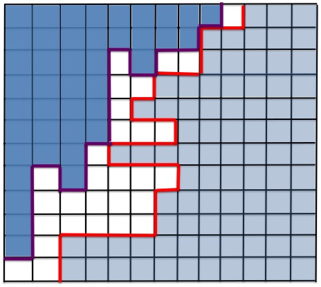
We next show that the resulting allocation regions have the shape of Figure 5, meaning that the borders of those regions consist a valid allocation pair. First notice that for any pair of valuations (x,y)𝑥𝑦(x,y) –including those for which xu(xϵ,yϵ)=1subscript𝑥𝑢𝑥italic-ϵ𝑦italic-ϵ1x_{u(\left\lfloor\frac{x}{\epsilon}\right\rfloor,\left\lfloor\frac{y}{\epsilon}\right\rfloor)}=1 and xv(xϵ,yϵ)=1subscript𝑥𝑣𝑥italic-ϵ𝑦italic-ϵ1x_{v(\left\lfloor\frac{x}{\epsilon}\right\rfloor,\left\lfloor\frac{y}{\epsilon}\right\rfloor)}=1– only one player gets allocated the item, so the non-crossing property is satisfied. To see why the regions are rightward and upward closed consider two nodes u(i,j)𝑢𝑖𝑗u(i,j) and u(i,j)𝑢superscript𝑖𝑗u(i^{\prime},j) on player 1’s grid, where i>isuperscript𝑖𝑖i^{\prime}>i. Notice that the set of nodes on player 2’s grid that node u(i,j)𝑢𝑖𝑗u(i,j) of player 1’s grid is connected to, is a strict superset of the nodes that node u(i,j)𝑢superscript𝑖𝑗u(i^{\prime},j) is connected to. Hence, if the maximum weight independent set includes node u(i,j)𝑢𝑖𝑗u(i,j) on the grid of player 1, it should also include u(i,j)𝑢superscript𝑖𝑗u(i^{\prime},j) for all values i>isuperscript𝑖𝑖i^{\prime}>i.

This gives us two stairwise curves which –although being a valid allocation pair– may fail to satisfy Condition 1, and hence may not be a feasible solution for Problem A𝐴A. To turn them into a proper valid pair, we can follow the same procedure as the one in the proof of Lemma 3.6 and come up with a feasible solution SOL(A)𝑆𝑂𝐿𝐴SOL(A) for Problem A𝐴A.

Because of the aforementioned transformation the cost of this solution is greater or equal to the cost of the optimal solution OPT(C)𝑂𝑃𝑇𝐶OPT(C) minus the contribution to the weight of the independent set by those nodes v(i,j)𝑣𝑖𝑗v(i,j) for which the corresponding node u(i,j)𝑢𝑖𝑗u(i,j) on the grid of player 1 is also included in the independent set. The reason for that is that for valuations (x,y)𝑥𝑦(x,y) such that xv(xϵ,yϵ)=1subscript𝑥𝑣𝑥italic-ϵ𝑦italic-ϵ1x_{v(\left\lfloor\frac{x}{\epsilon}\right\rfloor,\left\lfloor\frac{y}{\epsilon}\right\rfloor)}=1 and xu(xϵ,yϵ)=1subscript𝑥𝑢𝑥italic-ϵ𝑦italic-ϵ1x_{u(\left\lfloor\frac{x}{\epsilon}\right\rfloor,\left\lfloor\frac{y}{\epsilon}\right\rfloor)}=1, our solution explicitly allocates the item only to player 1, therefore losing the weight contribution of node v(xϵ,yϵ)𝑣𝑥italic-ϵ𝑦italic-ϵv(\left\lfloor\frac{x}{\epsilon}\right\rfloor,\left\lfloor\frac{y}{\epsilon}\right\rfloor). In what follows we argue that this results in the loss of an ϵitalic-ϵ\epsilon-additive factor, so that the cost of the resulting solution is at least:

uUxufd(u)+vVxvgd(v)ϵ=OPT(C)ϵsubscript𝑢𝑈subscript𝑥𝑢subscript𝑓𝑑𝑢subscript𝑣𝑉subscript𝑥𝑣subscript𝑔𝑑𝑣italic-ϵ𝑂𝑃𝑇𝐶italic-ϵ\sum_{u\in U}x_{u}f_{d}(u)+\sum_{v\in V}x_{v}g_{d}(v)-\epsilon=OPT(C)-\epsilon

To show this we first argue that the number of nodes v(i,j)𝑣𝑖𝑗v(i,j) for which this happens is small, in particular there can only be at most 1/ϵ1italic-ϵ1/\epsilon such nodes. To see this notice that in the constructed feasible solution to Problem A𝐴A, these nodes lie on the boundary between regions where player 1 gets the item and player 2 gets the item; any such boundary has to be monotone, since it corresponds to the overlap of the two allocation curves α,β𝛼𝛽\alpha,\beta, and it can therefore contain at most 1/ϵ1italic-ϵ1/\epsilon nodes. Next notice that the value of g𝑔g at any point (x,y)𝑥𝑦(x,y) is at most 1: indeed, g(x,y)𝑔𝑥𝑦g(x,y) is defined as yϕ(x,y)y1ϕ(x,t)𝑑t𝑦italic-ϕ𝑥𝑦superscriptsubscript𝑦1italic-ϕ𝑥𝑡differential-d𝑡y\phi(x,y)-\int_{y}^{1}\phi(x,t)dt, wherever y[maxyyyy1ϕ(x,t)𝑑t]𝑦delimited-[]subscriptsuperscript𝑦𝑦superscript𝑦superscriptsubscriptsuperscript𝑦1italic-ϕ𝑥𝑡differential-d𝑡\frac{\partial}{\partial y}\left[\max_{y^{\prime}\geq y}y^{\prime}\cdot\int_{y^{\prime}}^{1}\phi(x,t)\,dt\right] is defined, and extended to full range by right continuity. It follows immediately that g(x,y)1𝑔𝑥𝑦1g(x,y)\leq 1 and wv(i,j)=gd(i,j)ϵ2subscript𝑤𝑣𝑖𝑗subscript𝑔𝑑𝑖𝑗superscriptitalic-ϵ2w_{v(i,j)}=g_{d}(i,j)\leq\epsilon^{2}; therefore the total weight loss is at most 1ϵϵ21italic-ϵsuperscriptitalic-ϵ2\frac{1}{\epsilon}\cdot\epsilon^{2} and the lemma follows. ∎

Refer to caption
Figure 5: The solution for Problem A𝐴A prior to the transformation of Lemma 3.6.
Lemma 5.7.

For the optimal solutions of B𝐵B and D𝐷D we have: OPT(D)OPT(B)𝑂𝑃𝑇𝐷𝑂𝑃𝑇𝐵OPT(D)\geq OPT(B).

Proof.

Given a feasible solution for Problem D𝐷D, we will come up with a feasible solution of the same cost for Problem B𝐵B. The optimum solution for Problem B𝐵B will have at most that cost and the lemma follows.

We start by defining γ(x1,y1,x2,y2)𝛾subscript𝑥1subscript𝑦1subscript𝑥2subscript𝑦2\gamma(x_{1},y_{1},x_{2},y_{2}), for any pair of points (x1,y1),(x2,y2)subscript𝑥1subscript𝑦1subscript𝑥2subscript𝑦2(x_{1},y_{1}),(x_{2},y_{2}) where the ϵ2superscriptitalic-ϵ2\epsilon^{2}-area square containing (x2,y2)subscript𝑥2subscript𝑦2(x_{2},y_{2}) lies in the (strict) southeast orthant of the ϵ2superscriptitalic-ϵ2\epsilon^{2}-area square containing (x1,y1)subscript𝑥1subscript𝑦1(x_{1},y_{1}), as follows:

γ(x1,y1,x2,y2)=f(x1,y1)g(x2,y2)yuvwuwv,ifx1ϵ<x2ϵandy1ϵ>y2ϵ𝛾subscript𝑥1subscript𝑦1subscript𝑥2subscript𝑦2𝑓subscript𝑥1subscript𝑦1𝑔subscript𝑥2subscript𝑦2subscript𝑦𝑢𝑣subscript𝑤𝑢subscript𝑤𝑣ifsubscript𝑥1italic-ϵexpectationsubscript𝑥2italic-ϵandsubscript𝑦1italic-ϵsubscript𝑦2italic-ϵ\gamma(x_{1},y_{1},x_{2},y_{2})=f(x_{1},y_{1})\cdot g(x_{2},y_{2})\cdot\frac{y_{uv}}{w_{u}w_{v}},~{}~{}~{}~{}~{}\text{if}~{}~{}\left\lfloor\frac{x_{1}}{\epsilon}\right\rfloor<\left\lfloor\frac{x_{2}}{\epsilon}\right\rfloor~{}~{}\text{and}~{}~{}\left\lfloor\frac{y_{1}}{\epsilon}\right\rfloor>\left\lfloor\frac{y_{2}}{\epsilon}\right\rfloor

where uU𝑢𝑈u\in U (resp. vV𝑣𝑉v\in V) is the grid point u(x1ϵ,y1ϵ)𝑢subscript𝑥1italic-ϵsubscript𝑦1italic-ϵu\left(\left\lfloor\frac{x_{1}}{\epsilon}\right\rfloor,\left\lfloor\frac{y_{1}}{\epsilon}\right\rfloor\right) (resp. v(x2ϵ,y2ϵ)𝑣subscript𝑥2italic-ϵsubscript𝑦2italic-ϵv\left(\left\lfloor\frac{x_{2}}{\epsilon}\right\rfloor,\left\lfloor\frac{y_{2}}{\epsilon}\right\rfloor\right)) that corresponds to the little ϵ2superscriptitalic-ϵ2\epsilon^{2}-area square containing point (x1,y1)subscript𝑥1subscript𝑦1(x_{1},y_{1}) (resp. (x2,y2))(x_{2},y_{2})). Finally, we let:

γ(x1,y1,x2,y2)=0,ifx1ϵx2ϵory1ϵy2ϵformulae-sequence𝛾subscript𝑥1subscript𝑦1subscript𝑥2subscript𝑦20ifsubscript𝑥1italic-ϵsubscript𝑥2italic-ϵorsubscript𝑦1italic-ϵsubscript𝑦2italic-ϵ\gamma(x_{1},y_{1},x_{2},y_{2})=0,~{}~{}~{}~{}~{}\text{if}~{}~{}\left\lfloor\frac{x_{1}}{\epsilon}\right\rfloor\geq\left\lfloor\frac{x_{2}}{\epsilon}\right\rfloor~{}~{}\text{or}~{}~{}\left\lfloor\frac{y_{1}}{\epsilon}\right\rfloor\leq\left\lfloor\frac{y_{2}}{\epsilon}\right\rfloor

We next verify that the function γ𝛾\gamma defined above satisfies the constraints of Problem B𝐵B. Since the non-negativity constraint is obviously satisfied, we only need to check that γ𝛾\gamma satisfies the first and second constraints of Problem B𝐵B. We only provide the proof for the first constraint and the proof for the second constraint follows along the exact same lines:

0y1x11γ(x1,y1,x2,y2)𝑑x2𝑑y2superscriptsubscript0subscript𝑦1superscriptsubscriptsubscript𝑥11𝛾subscript𝑥1subscript𝑦1subscript𝑥2subscript𝑦2differential-dsubscript𝑥2differential-dsubscript𝑦2\displaystyle\int_{0}^{y_{1}}\int_{x_{1}}^{1}\gamma(x_{1},y_{1},x_{2},y_{2})\,dx_{2}\,dy_{2}
=\displaystyle= i>x1ϵ,j<y1ϵϵiϵ(i+1)ϵjϵ(j+1)f(x1,y1)g(x2,y2)yu(x1ϵ,y1ϵ),v(x2ϵ,y2ϵ)wu(x1ϵ,y1ϵ)wv(x2ϵ,y2ϵ)𝑑y2𝑑x2subscriptformulae-sequence𝑖subscript𝑥1italic-ϵ𝑗subscript𝑦1italic-ϵsuperscriptsubscriptitalic-ϵ𝑖italic-ϵ𝑖1superscriptsubscriptitalic-ϵ𝑗italic-ϵ𝑗1𝑓subscript𝑥1subscript𝑦1𝑔subscript𝑥2subscript𝑦2subscript𝑦𝑢subscript𝑥1italic-ϵsubscript𝑦1italic-ϵ𝑣subscript𝑥2italic-ϵsubscript𝑦2italic-ϵsubscript𝑤𝑢subscript𝑥1italic-ϵsubscript𝑦1italic-ϵsubscript𝑤𝑣subscript𝑥2italic-ϵsubscript𝑦2italic-ϵdifferential-dsubscript𝑦2differential-dsubscript𝑥2\displaystyle\sum_{i>\left\lfloor\frac{x_{1}}{\epsilon}\right\rfloor,j<\left\lfloor\frac{y_{1}}{\epsilon}\right\rfloor}\int_{\epsilon i}^{\epsilon(i+1)}\int_{\epsilon j}^{\epsilon(j+1)}f(x_{1},y_{1})\cdot g(x_{2},y_{2})\cdot\frac{y_{u\left(\left\lfloor\frac{x_{1}}{\epsilon}\right\rfloor,\left\lfloor\frac{y_{1}}{\epsilon}\right\rfloor\right),v\left(\left\lfloor\frac{x_{2}}{\epsilon}\right\rfloor,\left\lfloor\frac{y_{2}}{\epsilon}\right\rfloor\right)}}{w_{u\left(\left\lfloor\frac{x_{1}}{\epsilon}\right\rfloor,\left\lfloor\frac{y_{1}}{\epsilon}\right\rfloor\right)}\cdot w_{v\left(\left\lfloor\frac{x_{2}}{\epsilon}\right\rfloor,\left\lfloor\frac{y_{2}}{\epsilon}\right\rfloor\right)}}\,dy_{2}\,dx_{2}
=\displaystyle= f(x1,y1)i>x1ϵ,j<y1ϵyu(x1ϵ,y1ϵ),v(i,j)wu(x1ϵ,y1ϵ)wv(i,j)ϵiϵ(i+1)ϵjϵ(j+1)g(x2,y2)𝑑y2𝑑x2𝑓subscript𝑥1subscript𝑦1subscriptformulae-sequence𝑖subscript𝑥1italic-ϵ𝑗subscript𝑦1italic-ϵsubscript𝑦𝑢subscript𝑥1italic-ϵsubscript𝑦1italic-ϵ𝑣𝑖𝑗subscript𝑤𝑢subscript𝑥1italic-ϵsubscript𝑦1italic-ϵsubscript𝑤𝑣𝑖𝑗superscriptsubscriptitalic-ϵ𝑖italic-ϵ𝑖1superscriptsubscriptitalic-ϵ𝑗italic-ϵ𝑗1𝑔subscript𝑥2subscript𝑦2differential-dsubscript𝑦2differential-dsubscript𝑥2\displaystyle f(x_{1},y_{1})\cdot\sum_{i>\left\lfloor\frac{x_{1}}{\epsilon}\right\rfloor,j<\left\lfloor\frac{y_{1}}{\epsilon}\right\rfloor}\frac{y_{u\left(\left\lfloor\frac{x_{1}}{\epsilon}\right\rfloor,\left\lfloor\frac{y_{1}}{\epsilon}\right\rfloor\right),v(i,j)}}{w_{u\left(\left\lfloor\frac{x_{1}}{\epsilon}\right\rfloor,\left\lfloor\frac{y_{1}}{\epsilon}\right\rfloor\right)}\cdot w_{v(i,j)}}\cdot\int_{\epsilon i}^{\epsilon(i+1)}\int_{\epsilon j}^{\epsilon(j+1)}g(x_{2},y_{2})\,dy_{2}\,dx_{2}
=\displaystyle= f(x1,y1)i>x1ϵ,j<y1ϵyu(x1ϵ,y1ϵ),v(i,j)wu(x1ϵ,y1ϵ)wv(i,j)wv(i,j)𝑓subscript𝑥1subscript𝑦1subscriptformulae-sequence𝑖subscript𝑥1italic-ϵ𝑗subscript𝑦1italic-ϵsubscript𝑦𝑢subscript𝑥1italic-ϵsubscript𝑦1italic-ϵ𝑣𝑖𝑗subscript𝑤𝑢subscript𝑥1italic-ϵsubscript𝑦1italic-ϵsubscript𝑤𝑣𝑖𝑗subscript𝑤𝑣𝑖𝑗\displaystyle f(x_{1},y_{1})\cdot\sum_{i>\left\lfloor\frac{x_{1}}{\epsilon}\right\rfloor,j<\left\lfloor\frac{y_{1}}{\epsilon}\right\rfloor}\frac{y_{u\left(\left\lfloor\frac{x_{1}}{\epsilon}\right\rfloor,\left\lfloor\frac{y_{1}}{\epsilon}\right\rfloor\right),v(i,j)}}{w_{u\left(\left\lfloor\frac{x_{1}}{\epsilon}\right\rfloor,\left\lfloor\frac{y_{1}}{\epsilon}\right\rfloor\right)}\cdot w_{v(i,j)}}\cdot w_{v(i,j)}
=\displaystyle= f(x1,y1)i>x1ϵ,j<y1ϵyu(x1ϵ,y1ϵ),v(i,j)wu(x1ϵ,y1ϵ)𝑓subscript𝑥1subscript𝑦1subscriptformulae-sequence𝑖subscript𝑥1italic-ϵ𝑗subscript𝑦1italic-ϵsubscript𝑦𝑢subscript𝑥1italic-ϵsubscript𝑦1italic-ϵ𝑣𝑖𝑗subscript𝑤𝑢subscript𝑥1italic-ϵsubscript𝑦1italic-ϵ\displaystyle f(x_{1},y_{1})\cdot\sum_{i>\left\lfloor\frac{x_{1}}{\epsilon}\right\rfloor,j<\left\lfloor\frac{y_{1}}{\epsilon}\right\rfloor}\frac{y_{u\left(\left\lfloor\frac{x_{1}}{\epsilon}\right\rfloor,\left\lfloor\frac{y_{1}}{\epsilon}\right\rfloor\right),v(i,j)}}{w_{u\left(\left\lfloor\frac{x_{1}}{\epsilon}\right\rfloor,\left\lfloor\frac{y_{1}}{\epsilon}\right\rfloor\right)}}
\displaystyle\geq f(x1,y1)𝑓subscript𝑥1subscript𝑦1\displaystyle f(x_{1},y_{1})

where in the first equality we split the integration over discretized square regions of area ϵ2superscriptitalic-ϵ2\epsilon^{2} (the same that are used in the discrete auxiliary Problems C𝐶C and D𝐷D) and in the second equality we rearranged the order of summation and integration, noticing that the weights w𝑤w and flows y𝑦y remain constant across the discretized squares (independently of the actual value of (x2,y2)subscript𝑥2subscript𝑦2(x_{2},y_{2})). In the third equality we used the definition of the weight w𝑤w and in the last inequality we used the fact that y𝑦y is a feasible solution for Problem D𝐷D and therefore vEyuvwusubscript𝑣𝐸subscript𝑦𝑢𝑣subscript𝑤𝑢\sum_{v\in E}y_{uv}\geq w_{u}.

We conclude our proof by showing that the cost of the feasible solution we produced is exactly OPT(D)𝑂𝑃𝑇𝐷OPT(D):

01010y1x11γ(x1,y1,x2,y2)𝑑x2𝑑y2𝑑x1𝑑y1superscriptsubscript01superscriptsubscript01superscriptsubscript0subscript𝑦1superscriptsubscriptsubscript𝑥11𝛾subscript𝑥1subscript𝑦1subscript𝑥2subscript𝑦2differential-dsubscript𝑥2differential-dsubscript𝑦2differential-dsubscript𝑥1differential-dsubscript𝑦1\displaystyle\int_{0}^{1}\int_{0}^{1}\int_{0}^{y_{1}}\int_{x_{1}}^{1}\gamma(x_{1},y_{1},x_{2},y_{2})\,dx_{2}\,dy_{2}\,dx_{1}\,dy_{1}
=\displaystyle= i,jϵiϵ(i+1)ϵjϵ(j+1)0y1x11γ(x1,y1,x2,y2)𝑑x2𝑑y2𝑑x1𝑑y1subscript𝑖𝑗superscriptsubscriptitalic-ϵ𝑖italic-ϵ𝑖1superscriptsubscriptitalic-ϵ𝑗italic-ϵ𝑗1superscriptsubscript0subscript𝑦1superscriptsubscriptsubscript𝑥11𝛾subscript𝑥1subscript𝑦1subscript𝑥2subscript𝑦2differential-dsubscript𝑥2differential-dsubscript𝑦2differential-dsubscript𝑥1differential-dsubscript𝑦1\displaystyle\sum_{i,j}\int_{\epsilon i}^{\epsilon(i+1)}\int_{\epsilon j}^{\epsilon(j+1)}\int_{0}^{y_{1}}\int_{x_{1}}^{1}\gamma(x_{1},y_{1},x_{2},y_{2})\,dx_{2}\,dy_{2}\,dx_{1}\,dy_{1}
=\displaystyle= i,jϵiϵ(i+1)ϵjϵ(j+1)f(x1,y1)i>x1ϵ,j<y1ϵyu(x1ϵ,y1ϵ),v(i,j)wu(x1ϵ,y1ϵ)dx1dy1subscript𝑖𝑗superscriptsubscriptitalic-ϵ𝑖italic-ϵ𝑖1superscriptsubscriptitalic-ϵ𝑗italic-ϵ𝑗1𝑓subscript𝑥1subscript𝑦1subscriptformulae-sequencesuperscript𝑖subscript𝑥1italic-ϵsuperscript𝑗subscript𝑦1italic-ϵsubscript𝑦𝑢subscript𝑥1italic-ϵsubscript𝑦1italic-ϵ𝑣superscript𝑖superscript𝑗subscript𝑤𝑢subscript𝑥1italic-ϵsubscript𝑦1italic-ϵ𝑑subscript𝑥1𝑑subscript𝑦1\displaystyle\sum_{i,j}\int_{\epsilon i}^{\epsilon(i+1)}\int_{\epsilon j}^{\epsilon(j+1)}f(x_{1},y_{1})\cdot\sum_{i^{\prime}>\left\lfloor\frac{x_{1}}{\epsilon}\right\rfloor,j^{\prime}<\left\lfloor\frac{y_{1}}{\epsilon}\right\rfloor}\frac{y_{u\left(\left\lfloor\frac{x_{1}}{\epsilon}\right\rfloor,\left\lfloor\frac{y_{1}}{\epsilon}\right\rfloor\right),v(i^{\prime},j^{\prime})}}{w_{u\left(\left\lfloor\frac{x_{1}}{\epsilon}\right\rfloor,\left\lfloor\frac{y_{1}}{\epsilon}\right\rfloor\right)}}\,dx_{1}\,dy_{1}
=\displaystyle= i,ji>i,j<jyu(i,j),v(i,j)wu(i,j)ϵiϵ(i+1)ϵjϵ(j+1)f(x1,y1)𝑑x1𝑑y1subscript𝑖𝑗subscriptformulae-sequencesuperscript𝑖𝑖superscript𝑗𝑗subscript𝑦𝑢𝑖𝑗𝑣superscript𝑖superscript𝑗subscript𝑤𝑢𝑖𝑗superscriptsubscriptitalic-ϵ𝑖italic-ϵ𝑖1superscriptsubscriptitalic-ϵ𝑗italic-ϵ𝑗1𝑓subscript𝑥1subscript𝑦1differential-dsubscript𝑥1differential-dsubscript𝑦1\displaystyle\sum_{i,j}\sum_{i^{\prime}>i,j^{\prime}<j}\frac{y_{u(i,j),v(i^{\prime},j^{\prime})}}{w_{u(i,j)}}\cdot\int_{\epsilon i}^{\epsilon(i+1)}\int_{\epsilon j}^{\epsilon(j+1)}f(x_{1},y_{1})\,dx_{1}\,dy_{1}
=\displaystyle= i,ji>i,j<jyu(i,j),v(i,j)wu(i,j)wu(i,j)subscript𝑖𝑗subscriptformulae-sequencesuperscript𝑖𝑖superscript𝑗𝑗subscript𝑦𝑢𝑖𝑗𝑣superscript𝑖superscript𝑗subscript𝑤𝑢𝑖𝑗subscript𝑤𝑢𝑖𝑗\displaystyle\sum_{i,j}\sum_{i^{\prime}>i,j^{\prime}<j}\frac{y_{u(i,j),v(i^{\prime},j^{\prime})}}{w_{u(i,j)}}\cdot w_{u(i,j)}
=\displaystyle= i,ji>i,j<jyu(i,j),v(i,j)subscript𝑖𝑗subscriptformulae-sequencesuperscript𝑖𝑖superscript𝑗𝑗subscript𝑦𝑢𝑖𝑗𝑣superscript𝑖superscript𝑗\displaystyle\sum_{i,j}\sum_{i^{\prime}>i,j^{\prime}<j}y_{u(i,j),v(i^{\prime},j^{\prime})}
=\displaystyle= OPT(D)𝑂𝑃𝑇𝐷\displaystyle OPT(D)

where in the first equality we split the integration of (x1,y1)subscript𝑥1subscript𝑦1(x_{1},y_{1}) over discretized square regions of area ϵ2superscriptitalic-ϵ2\epsilon^{2} and in the second equality we plugged in the expression for 0y1x11γ(x1,y1,x2,y2)𝑑x2𝑑y2superscriptsubscript0subscript𝑦1superscriptsubscriptsubscript𝑥11𝛾subscript𝑥1subscript𝑦1subscript𝑥2subscript𝑦2differential-dsubscript𝑥2differential-dsubscript𝑦2\int_{0}^{y_{1}}\int_{x_{1}}^{1}\gamma(x_{1},y_{1},x_{2},y_{2})\,dx_{2}\,dy_{2} that we had derived from our previous proof establishing that the first constraint of Problem B𝐵B was satisfied. In the third equality we once again rearranged the order of summation and integration, noticing that the weights w𝑤w and flows y𝑦y remain constant across the discretized squares (independently of the actual value of (x1,y1)subscript𝑥1subscript𝑦1(x_{1},y_{1})), in the fourth equality we used the definition of the weight w𝑤w and in the last equality we replaced with the objective function of Problem D𝐷D.

Proof of the Duality Theorem.

First notice that, by strong duality and since the constraint matrix of Problem C is totally unimodular, we have that OPT(C)=OPT(D)𝑂𝑃𝑇𝐶𝑂𝑃𝑇𝐷OPT(C)=OPT(D); combining this with Lemmas 5.6 and 5.7 we get OPT(A)OPT(B)ϵ𝑂𝑃𝑇𝐴𝑂𝑃𝑇𝐵italic-ϵOPT(A)\geq OPT(B)-\epsilon. From Lemma 5.5 we get OPT(A)OPT(B)𝑂𝑃𝑇𝐴𝑂𝑃𝑇𝐵OPT(A)\leq OPT(B). By having ϵ0italic-ϵ0\epsilon\rightarrow 0 we get the result. ∎

5.2 The Algorithm

The proof of the Main Theorem suggests a fully polynomial-time approximation scheme (FPTAS) for the continuous case, that is, a mechanism that approximates the optimal profit within additive error ϵitalic-ϵ\epsilon, and runs in time polynomial in 1ϵ1italic-ϵ1\over\epsilon. In the algorithm and the correctness proof, we assume that the continuous joint distribution ϕitalic-ϕ\phi is Lipschitz continuous, and that it is presented through oracle access. It is easy to see that these assumptions are essentially necessary, in that no approximation (or meaningful solution of any other nature) is possible when the function can be arbitrarily discontinuous, or is inaccessible for large parts of the domain.

Algorithm 1 OptimalAuction for two bidders with continuous distributions
1:Input: probability distribution ϕ[0,1]2italic-ϕsuperscript012\phi\in[0,1]^{2}
2:Compute f(,),g(,)𝑓𝑔f(\cdot,\cdot),g(\cdot,\cdot)
3:Discretize the unit plane and construct the bipartite graph G𝐺G as described in Section 5.1
4:Compute a Maximum Weight Independent Set for G𝐺G
5:Output: (α,β)𝛼𝛽(\alpha,\beta), the valid allocation pair corresponding to the stair-like curves of Figure 5

The following theorem establishes that our algorithm has the desired properties.

Theorem 5.8.

Algorithm 1 returns a truthful mechanism that approximates the optimal profit within ϵitalic-ϵ\epsilon additive error; moreover the algorithm runs in time polynomial in 1/ϵ1italic-ϵ1/\epsilon.

Proof.

Algorithm 1 returns a valid allocation pair so it is truthful by construction. However the allocation pair (α,β)𝛼𝛽(\alpha,\beta) returned may well not satisfy condition (1) and may consequently not constitute a feasible solution to Problem A. This is problematic since it does not allow us to use Lemma 3.4 to compute the profit of the auction returned. To that end we need to establish that the violation of condition (1) is –in some sense– negligible; we do that next.

Suppose that curve α(y)𝛼𝑦\alpha(y) violates condition (1) for some y[0,1]superscript𝑦01y^{\ast}\in[0,1] and let

x=argmaxxα(y)xx1ϕ(t,y)𝑑t,superscript𝑥subscript𝑥𝛼superscript𝑦𝑥superscriptsubscript𝑥1italic-ϕ𝑡superscript𝑦differential-d𝑡x^{\ast}=\arg\max_{x\geq\alpha(y^{\ast})}x\cdot\int_{x}^{1}\phi(t,y^{\ast})\,dt,

be the minimum x𝑥x for which we could create a new solution αsuperscript𝛼\alpha^{\prime} by setting α(y)=xsuperscript𝛼superscript𝑦superscript𝑥\alpha^{\prime}(y^{\ast})=x^{\ast} and have condition (1) restored, while not altering the profit of our auction.111The reader is referred to Lemma 3.6 for further discussion on this point. We will argue that

α(y)α(y)1ϕ(t,y)𝑑txx1ϕ(t,y)𝑑tΘ(ϵ)𝛼superscript𝑦superscriptsubscript𝛼superscript𝑦1italic-ϕ𝑡superscript𝑦differential-d𝑡superscript𝑥superscriptsubscriptsuperscript𝑥1italic-ϕ𝑡superscript𝑦differential-d𝑡Θitalic-ϵ\alpha(y^{\ast})\cdot\int_{\alpha(y^{\ast})}^{1}\phi(t,y^{\ast})\,dt\geq x^{\ast}\cdot\int_{x^{\ast}}^{1}\phi(t,y^{\ast})\,dt-\Theta(\epsilon) (2)

To do that we consider the node corresponding to the little square on the unit plane containing (α(y),y)𝛼superscript𝑦superscript𝑦(\alpha(y^{\ast}),y^{\ast}). Since this node belongs to the boundary of the allocation region of player 1, we can assume wlog that it has non-zero weight; hence there must exist some point (x1,y1)subscript𝑥1subscript𝑦1(x_{1},y_{1}) in the corresponding square on the unit plane with f(x1,y1)>0𝑓subscript𝑥1subscript𝑦10f(x_{1},y_{1})>0. By the definition of f𝑓f this immediately implies that

x1x11ϕ(t,y1)𝑑txx1ϕ(t,y1)𝑑t,for all xx1formulae-sequencesubscript𝑥1superscriptsubscriptsubscript𝑥11italic-ϕ𝑡subscript𝑦1differential-d𝑡𝑥superscriptsubscript𝑥1italic-ϕ𝑡subscript𝑦1differential-d𝑡for all 𝑥subscript𝑥1x_{1}\cdot\int_{x_{1}}^{1}\phi(t,y_{1})\,dt\geq x\cdot\int_{x}^{1}\phi(t,y_{1})\,dt,~{}~{}~{}~{}\text{for all }x\geq x_{1}

and therefore in particular that

x1x11ϕ(t,y1)𝑑txx1ϕ(t,y1)𝑑t.subscript𝑥1superscriptsubscriptsubscript𝑥11italic-ϕ𝑡subscript𝑦1differential-d𝑡superscript𝑥superscriptsubscriptsuperscript𝑥1italic-ϕ𝑡subscript𝑦1differential-d𝑡x_{1}\cdot\int_{x_{1}}^{1}\phi(t,y_{1})\,dt\geq x^{\ast}\cdot\int_{x^{\ast}}^{1}\phi(t,y_{1})\,dt. (3)

Since the l1subscript𝑙1l_{1}-distance of points (α(y),y)𝛼superscript𝑦superscript𝑦(\alpha(y^{\ast}),y^{\ast}) and (x1,y1)subscript𝑥1subscript𝑦1(x_{1},y_{1}) and of points (x,y)superscript𝑥superscript𝑦(x^{\ast},y^{\ast}) and (x,y1)superscript𝑥subscript𝑦1(x^{\ast},y_{1}) is at most 2ϵ2italic-ϵ2\epsilon, we get that:

α(y)α(y)1ϕ(t,y)𝑑tx1α(x1)1ϕ(t,y1)𝑑t2λϵxx1ϕ(t,y1)𝑑t2λϵxx1ϕ(t,y)𝑑t4λϵ𝛼superscript𝑦superscriptsubscript𝛼superscript𝑦1italic-ϕ𝑡superscript𝑦differential-d𝑡subscript𝑥1superscriptsubscript𝛼subscript𝑥11italic-ϕ𝑡subscript𝑦1differential-d𝑡2𝜆italic-ϵsuperscript𝑥superscriptsubscriptsuperscript𝑥1italic-ϕ𝑡subscript𝑦1differential-d𝑡2𝜆italic-ϵsuperscript𝑥superscriptsubscriptsuperscript𝑥1italic-ϕ𝑡superscript𝑦differential-d𝑡4𝜆italic-ϵ\alpha(y^{\ast})\cdot\int_{\alpha(y^{\ast})}^{1}\phi(t,y^{\ast})\,dt\geq x_{1}\cdot\int_{\alpha(x_{1})}^{1}\phi(t,y_{1})\,dt-2\lambda\epsilon\geq x^{\ast}\cdot\int_{x^{\ast}}^{1}\phi(t,y_{1})\,dt-2\lambda\epsilon\geq x^{\ast}\cdot\int_{x^{\ast}}^{1}\phi(t,y^{\ast})\,dt-4\lambda\epsilon

where in the first and third inequalities we used the fact that xx1ϕ(t,y)𝑑t𝑥superscriptsubscript𝑥1italic-ϕ𝑡𝑦differential-d𝑡x\cdot\int_{x}^{1}\phi(t,y)\,dt is Lipschitz-continuous for some constant λ𝜆\lambda and in the second inequality we used inequality (3). The exact same argument applies for β(x)𝛽𝑥\beta(x) as well.

We are now ready to prove a lower bound on the profit of the auction returned by our algorithm; in what follows we use α(y)superscript𝛼𝑦\alpha^{\prime}(y) and β(x)superscript𝛽𝑥\beta^{\prime}(x) to denote the allocation curves that would result by the aforementioned transformation. Note that by construction it holds that

α(y)α(y)1ϕ(x,y)𝑑x=α(y)1f(x,y)𝑑xandβ(x)β(x)1ϕ(x,y)𝑑y=β(x)1g(x,y)𝑑ysuperscript𝛼𝑦superscriptsubscriptsuperscript𝛼𝑦1italic-ϕ𝑥𝑦differential-d𝑥superscriptsubscriptsuperscript𝛼𝑦1𝑓𝑥𝑦differential-d𝑥andsuperscript𝛽𝑥superscriptsubscriptsuperscript𝛽𝑥1italic-ϕ𝑥𝑦differential-d𝑦superscriptsubscriptsuperscript𝛽𝑥1𝑔𝑥𝑦differential-d𝑦\alpha^{\prime}(y)\cdot\int_{\alpha^{\prime}(y)}^{1}\phi(x,y)\,dx=\int_{\alpha^{\prime}(y)}^{1}f(x,y)\,dx~{}~{}~{}\text{and}~{}~{}~{}\beta^{\prime}(x)\cdot\int_{\beta^{\prime}(x)}^{1}\phi(x,y)\,dy=\int_{\beta^{\prime}(x)}^{1}g(x,y)\,dy (4)

so the profit of the algorithm is:

01[α(y)α(y)1ϕ(x,y)𝑑x]𝑑y+01[β(x)β(x)1ϕ(x,y)𝑑y]𝑑xsuperscriptsubscript01delimited-[]𝛼𝑦superscriptsubscript𝛼𝑦1italic-ϕ𝑥𝑦differential-d𝑥differential-d𝑦superscriptsubscript01delimited-[]𝛽𝑥superscriptsubscript𝛽𝑥1italic-ϕ𝑥𝑦differential-d𝑦differential-d𝑥\displaystyle\int_{0}^{1}\left[\alpha(y)\cdot\int_{\alpha(y)}^{1}\phi(x,y)\,dx\right]\,dy+\int_{0}^{1}\left[\beta(x)\cdot\int_{\beta(x)}^{1}\phi(x,y)\,dy\right]\,dx
\displaystyle\geq 01[α(y)α(y)1ϕ(x,y)𝑑xΘ(ϵ)]𝑑y+01[β(x)β(x)1ϕ(x,y)𝑑yΘ(ϵ)]𝑑xsuperscriptsubscript01delimited-[]superscript𝛼𝑦superscriptsubscriptsuperscript𝛼𝑦1italic-ϕ𝑥𝑦differential-d𝑥Θitalic-ϵdifferential-d𝑦superscriptsubscript01delimited-[]superscript𝛽𝑥superscriptsubscriptsuperscript𝛽𝑥1italic-ϕ𝑥𝑦differential-d𝑦Θitalic-ϵdifferential-d𝑥\displaystyle\int_{0}^{1}\left[\alpha^{\prime}(y)\cdot\int_{\alpha^{\prime}(y)}^{1}\phi(x,y)\,dx-\Theta(\epsilon)\right]\,dy+\int_{0}^{1}\left[\beta^{\prime}(x)\cdot\int_{\beta^{\prime}(x)}^{1}\phi(x,y)\,dy-\Theta(\epsilon)\right]\,dx
=\displaystyle= 01α(y)1f(x,y)𝑑x𝑑y+01β(x)1g(x,y)𝑑y𝑑xΘ(ϵ)superscriptsubscript01superscriptsubscriptsuperscript𝛼𝑦1𝑓𝑥𝑦differential-d𝑥differential-d𝑦superscriptsubscript01superscriptsubscriptsuperscript𝛽𝑥1𝑔𝑥𝑦differential-d𝑦differential-d𝑥Θitalic-ϵ\displaystyle\int_{0}^{1}\int_{\alpha^{\prime}(y)}^{1}f(x,y)\,dx\,dy+\int_{0}^{1}\int_{\beta^{\prime}(x)}^{1}g(x,y)\,dy\,dx-\Theta(\epsilon)
=\displaystyle= OPT(C)Θ(ϵ)𝑂𝑃𝑇𝐶Θitalic-ϵ\displaystyle OPT(C)-\Theta(\epsilon)
\displaystyle\geq OPT(A)Θ(ϵ)𝑂𝑃𝑇𝐴Θitalic-ϵ\displaystyle OPT(A)-\Theta(\epsilon)

where in the first inequality we used inequality (2), in the first equality we used (4) and in the last inequality we used our Main Theorem from the previous section.

In terms of running time, the discretized approximations of f𝑓f and g𝑔g are trivial (because of Lipschitz continuity, we can take f(i,j)=f(iϵ,jϵ)𝑓𝑖𝑗𝑓𝑖italic-ϵ𝑗italic-ϵf(i,j)=f(i\epsilon,j\epsilon), and similarly for g𝑔g). Solving the Maximum Weight Independent Set problem is done exactly as in the previous section. ∎

6 NP-completeness

We show that for 3 bidders the problem of designing an approximately optimal (deterministic) auction becomes NP-hard. The current proof establishes hardness for a small threshold around 0.05%; we believe that this will not be too hard to improve upon.

6.1 A geometric characterization for three bidders

We start by formally defining the discrete version of the problem we will prove to be NP-hard; to simplify the exposition of the problem, we assume that the support of the discrete distribution is 𝒢=[S]×[S]×[S]𝒢delimited-[]𝑆delimited-[]𝑆delimited-[]𝑆\mathcal{G}=[S]\times[S]\times[S]. We are interested in this problem:

Definition 6.1 (3OptimalAuctionDesign).

Given a joint discrete probability distribution ϕitalic-ϕ\phi supported on 𝒢𝒢\mathcal{G}, find the optimal, ex-post IC and IR deterministic auction, denoted by a 3-dimensional allocation matrix A𝐴A, where A[x,y,z]=i𝐴𝑥𝑦𝑧𝑖A[x,y,z]=i, with i𝑖i being the index of the bidder who gets the item when the bid vector is (x,y,z)𝑥𝑦𝑧(x,y,z), or 0 if the auctioneer keeps the item.

As was the case with 2 bidders, the following notion of marginal profit contribution, appropriately modified for the discrete case, will be useful to our proof.

Definition 6.2.

The discrete analogues of the marginal profit contribution functions (Definition 3.2) for each player are the following:

f(x,y,z)=max{xxxϕ(x,y,z)x>xf(x,y,z),0}for player 1𝑓𝑥𝑦𝑧𝑥subscriptsuperscript𝑥𝑥italic-ϕsuperscript𝑥𝑦𝑧subscriptsuperscript𝑥𝑥𝑓superscript𝑥𝑦𝑧0for player 1f(x,y,z)=\max\left\{x\cdot\sum_{x^{\prime}\geq x}\phi(x^{\prime},y,z)-\sum_{x^{\prime}>x}f(x^{\prime},y,z),0\right\}~{}~{}\text{for player 1}
g(x,y,z)=max{yyyϕ(x,y,z)y>yf(x,y,z),0}for player 2𝑔𝑥𝑦𝑧𝑦subscriptsuperscript𝑦𝑦italic-ϕ𝑥superscript𝑦𝑧subscriptsuperscript𝑦𝑦𝑓𝑥superscript𝑦𝑧0for player 2g(x,y,z)=\max\left\{y\cdot\sum_{y^{\prime}\geq y}\phi(x,y^{\prime},z)-\sum_{y^{\prime}>y}f(x,y^{\prime},z),0\right\}~{}~{}\text{for player 2}
h(x,y,z)=max{zzzϕ(x,y,z)z>zf(x,y,z),0}for player 3𝑥𝑦𝑧𝑧subscriptsuperscript𝑧𝑧italic-ϕ𝑥𝑦superscript𝑧subscriptsuperscript𝑧𝑧𝑓𝑥𝑦superscript𝑧0for player 3h(x,y,z)=\max\left\{z\cdot\sum_{z^{\prime}\geq z}\phi(x,y,z^{\prime})-\sum_{z^{\prime}>z}f(x,y,z^{\prime}),0\right\}~{}~{}\text{for player 3}

The Segments.

Given a distribution ϕ(x,y,z)italic-ϕ𝑥𝑦𝑧\phi(x,y,z) over the points of 𝒢𝒢\mathcal{G}, any node (x,y,z)𝑥𝑦𝑧(x,y,z) of 𝒢𝒢\mathcal{G} with f(x,y,z)>0𝑓𝑥𝑦𝑧0f(x,y,z)>0 is the starting point of what we shall henceforth be calling an x𝑥x-segment: an interval (sequence of points) starting at node (x,y,z)𝑥𝑦𝑧(x,y,z) and including all nodes (x,y,z)superscript𝑥𝑦𝑧(x^{\prime},y,z) with xxsuperscript𝑥𝑥x^{\prime}\geq x. The weight of this segment is xxf(x,y,z)subscriptsuperscript𝑥𝑥𝑓superscript𝑥𝑦𝑧\sum_{x^{\prime}\geq x}f(x^{\prime},y,z). We define segments across the other dimensions analogously. The following problem222The reader may notice that the 3Segments problem is a maximum weight independent set problem in disguise. is essentially equivalent to the auction design problem:

Definition 6.3 (3Segments).

Given a joint discrete probability distribution ϕitalic-ϕ\phi supported on 𝒢𝒢\mathcal{G}, which induces a set of segments on 𝒢𝒢\mathcal{G} as described above, find a subset of non-intersecting segments with maximum sum of weights.

Lemma 6.4.

The problem 3Segments(ϕitalic-ϕ\phi) is equivalent to 3OptimalAuctionDesign(ϕ)italic-ϕ(\phi) via approximation-preserving reductions.

Proof.

(Sketch:) The correspondence between solutions of the two problems is rather immediate, with the x𝑥x-segment (respectively, y𝑦y-segment, z𝑧z-segment) at point (x,y,z)𝑥𝑦𝑧(x,y,z) included in the output set of segments if and only if A[x,y,z]=1𝐴𝑥𝑦𝑧1A[x,y,z]=1 (respectively, 2, 3) and A[x,y,z]=0𝐴superscript𝑥𝑦𝑧0A[x^{\prime},y,z]=0 for all x<xsuperscript𝑥𝑥x^{\prime}<x (respectively, A[x,y,z]=0𝐴𝑥superscript𝑦𝑧0A[x,y^{\prime},z]=0 for all y<ysuperscript𝑦𝑦y^{\prime}<y and A[x,y,z]=0𝐴𝑥𝑦superscript𝑧0A[x,y,z^{\prime}]=0 for all z<zsuperscript𝑧𝑧z^{\prime}<z). ∎

6.2 The construction

It suffices to show that 3Segments is NP-hard to approximate for some constant; we do that by reducing from 3CatSat, a special case of 3Sat:

Definition 6.5.

Let 3CatSat be the 3Sat problem with the input formula restricted to be of the following form. We have three types (categories) of variables {xi}i=1nx,{yi}i=1nysubscriptsubscript𝑥𝑖𝑖1subscript𝑛𝑥subscriptsubscript𝑦𝑖𝑖1subscript𝑛𝑦\{x_{i}\}_{i=1\ldots n_{x}},\{y_{i}\}_{i=1\ldots n_{y}} and {zi}i=1nzsubscriptsubscript𝑧𝑖𝑖1subscript𝑛𝑧\{z_{i}\}_{i=1\ldots n_{z}}, i.e. a total of n=nx+ny+nz𝑛subscript𝑛𝑥subscript𝑛𝑦subscript𝑛𝑧n=n_{x}+n_{y}+n_{z} variables, and m𝑚m clauses of the following form: every clause has at most one literal from every type (e.g. (x2¯y3¯z1)¯subscript𝑥2¯subscript𝑦3subscript𝑧1(\bar{x_{2}}\vee\bar{y_{3}}\vee z_{1}) or (x5¯z7)¯subscript𝑥5subscript𝑧7(\bar{x_{5}}\vee z_{7})).

Lemma 6.6.

3CatSat is NP-hard to approximate better than 79/80.

Proof.

We reduce from Max3Sat. In order to turn an instance of Max3Sat to an instance of 3CatSat it suffices to create three copies for every occurrence of a variable: for variable x𝑥x we create x1,x2,x3subscript𝑥1subscript𝑥2subscript𝑥3x_{1},x_{2},x_{3} and include the clauses (x¯1x2),(x¯2x3),(x¯3x1)subscript¯𝑥1subscript𝑥2subscript¯𝑥2subscript𝑥3subscript¯𝑥3subscript𝑥1(\overline{x}_{1}\lor x_{2}),(\overline{x}_{2}\lor x_{3}),(\overline{x}_{3}\lor x_{1}). This increases the number of clauses by at most 3n¯3¯𝑛3\bar{n}, where n¯¯𝑛\bar{n} is the number of literals in the formula. Given that Max3Sat is hard to approximate better than 7/8, it follows immediately that 3CatSat is hard to approximate better than 7/8m+3n¯m+3n¯78𝑚3¯𝑛𝑚3¯𝑛\frac{7/8m+3\bar{n}}{m+3\bar{n}}. Noticing that n¯3m¯𝑛3𝑚\bar{n}\leq 3m we get the desired approximation factor as an upper bound on this expression by picking n¯=3m¯𝑛3𝑚\bar{n}=3m. ∎

We start with some intuition about the reduction. The instance of 3Segments we create has three types of segments: literal segments, clause segments and scaffolding segments.

  • Literal segments are used to model truth assignments on variables; they ensure that every variable is assigned exactly one of the two possible truth values and that this assignment is consistent across all appearances of literals of this particular variable.

  • Clause segments model the truth assignment to literals of a particular clause; we create one such clause segment for every literal that appears in a clause and we make them intersect with the literal segments of those literals; the idea is that if the clause is satisfied we will be able to pick at least one clause segment per clause because the corresponding literal segment will not be picked. Moreover, we cannot pick two or more clause segments per clause, since they will all intersect with each other.

  • Scaffolding segments333Rather, scaffolding points, as these segments have zero length. ensure that, for some points, there are literal or clause segments that extend only to one of the three possible directions: In particular, given some point (x,y,z)𝑥𝑦𝑧(x,y,z) with positive marginal profit contribution for more than one players (for example when f(x,y,z)>0𝑓𝑥𝑦𝑧0f(x,y,z)>0 and g(x,y,z)>0𝑔𝑥𝑦𝑧0g(x,y,z)>0) we may want to have only x𝑥x or only y𝑦y-segments starting from (x,y,z)𝑥𝑦𝑧(x,y,z); scaffolding points make sure this is the case.

We show how to construct a probability distribution ϕitalic-ϕ\phi that serves as the input of 3Segments, given an instance of 3CatSat. In what follows we use n^^𝑛\hat{n} to denote max{nx,ny,nz}subscript𝑛𝑥subscript𝑛𝑦subscript𝑛𝑧\max\{n_{x},n_{y},n_{z}\}. The support444The support is actually a subset of this; these are all the points (values of the players) with potentially non-zero probabilities. This will become clear in the actual construction. of ϕitalic-ϕ\phi is: {h(i)|i=1,,n^+2m+4}3superscriptconditional-set𝑖𝑖1^𝑛2𝑚43\left\{h(i)|i=1,\ldots,\hat{n}+2m+4\right\}^{3}, for an appropriate choice of the values h(i)𝑖h(i) which we will fix later; for now all we assume is that hh is an increasing function of i𝑖i. The size of the support is at most (n^+2m+4)3superscript^𝑛2𝑚43(\hat{n}+2m+4)^{3}, so this is clearly a polynomial time construction.

We shall abuse notation and write ϕ(x,y,z)italic-ϕ𝑥𝑦𝑧\phi(x,y,z) instead of ϕ(h(x),h(y),h(z))italic-ϕ𝑥𝑦𝑧\phi\left(h(x),h(y),h(z)\right) when there is no ambiguity. We shall also refer to the sub-matrices ϕ(i,,),ϕ(,j,),ϕ(,,k)italic-ϕ𝑖italic-ϕ𝑗italic-ϕ𝑘\phi(i,\cdot,\cdot),\phi(\cdot,j,\cdot),\phi(\cdot,\cdot,k) as the “planes” x=i,y=jformulae-sequence𝑥𝑖𝑦𝑗x=i,y=j and z=k𝑧𝑘z=k respectively.

The construction goes as follows: we start with an all-zero matrix ϕitalic-ϕ\phi of the above size. Consider an arbitrary ordering of the clauses 111 through m𝑚m. Suppose the l𝑙l-th clause is of the form (xiyjzk)subscript𝑥𝑖subscript𝑦𝑗subscript𝑧𝑘(x_{i}\vee y_{j}\vee z_{k}) where xi,yjsubscript𝑥𝑖subscript𝑦𝑗x_{i},y_{j} and zksubscript𝑧𝑘z_{k} can be either positive or negative literals, and i(resp. j,k)=1,,nx(resp. ny,nz)𝑖resp. 𝑗𝑘1subscript𝑛𝑥resp. subscript𝑛𝑦subscript𝑛𝑧i\,\,(\text{resp. }j,k)=1,\ldots,n_{x}\,\,(\text{resp. }n_{y},n_{z}) (the same construction also works for clauses with less than 3 variables). For this clause we introduce the following literal segments (1,2,3) and clause segments (4). In what follows we will first set the probability mass of the point that is the apex of each segment, and will later show how to use scaffolding-points to ensure that there is only one segment starting at each such point, towards the appropriate direction.

  1. 1.

    If pos(xi)𝑝𝑜𝑠subscript𝑥𝑖pos(x_{i}) then ϕ(i+1,n^+2,n^+2+l)=c1italic-ϕ𝑖1^𝑛2^𝑛2𝑙subscript𝑐1\phi\left(i+1,\hat{n}+2,\hat{n}+2+l\right)=c_{1} and ϕ(i+1,n^+2+m+l,n^+2)=c1italic-ϕ𝑖1^𝑛2𝑚𝑙^𝑛2subscript𝑐1\phi\left(i+1,\hat{n}+2+m+l,\hat{n}+2\right)=c_{1}

    (These points are intended to be the apices of a y𝑦y-segment and a z𝑧z-segment respectively.)

    else ϕ(i+1,n^+2+l,n^+2)=c1italic-ϕ𝑖1^𝑛2𝑙^𝑛2subscript𝑐1\phi\left(i+1,\hat{n}+2+l,\hat{n}+2\right)=c_{1} and ϕ(i+1,n^+2,n^+2+m+l)=c1italic-ϕ𝑖1^𝑛2^𝑛2𝑚𝑙subscript𝑐1\phi\left(i+1,\hat{n}+2,\hat{n}+2+m+l\right)=c_{1}

    (These points are intended to be the apices of a z𝑧z-segment and a y𝑦y-segment respectively.)

  2. 2.

    If pos(yj)𝑝𝑜𝑠subscript𝑦𝑗pos(y_{j}) then ϕ(n^+2+l,j+1,n^+2)=c1italic-ϕ^𝑛2𝑙𝑗1^𝑛2subscript𝑐1\phi\left(\hat{n}+2+l,j+1,\hat{n}+2\right)=c_{1} and ϕ(n^+2,j+1,n^+2+m+l)=c1italic-ϕ^𝑛2𝑗1^𝑛2𝑚𝑙subscript𝑐1\phi\left(\hat{n}+2,j+1,\hat{n}+2+m+l\right)=c_{1},

    (These points are intended to be the apices of a z𝑧z-segment and an x𝑥x-segment respectively.)

    else ϕ(n^+2,j+1,n^+2+l)=c1italic-ϕ^𝑛2𝑗1^𝑛2𝑙subscript𝑐1\phi\left(\hat{n}+2,j+1,\hat{n}+2+l\right)=c_{1} and ϕ(n^+2+m+l,j+1,n^+2)=c1italic-ϕ^𝑛2𝑚𝑙𝑗1^𝑛2subscript𝑐1\phi\left(\hat{n}+2+m+l,j+1,\hat{n}+2\right)=c_{1}

    (These points are intended to be the apices of an x𝑥x-segment and a z𝑧z-segment respectively.)

  3. 3.

    If pos(zk)𝑝𝑜𝑠subscript𝑧𝑘pos(z_{k}) then ϕ(n^+2,n^+2+l,k+1)=c1italic-ϕ^𝑛2^𝑛2𝑙𝑘1subscript𝑐1\phi\left(\hat{n}+2,\hat{n}+2+l,k+1\right)=c_{1} and ϕ(n^+2+m+l,n^+2,k+1)=c1italic-ϕ^𝑛2𝑚𝑙^𝑛2𝑘1subscript𝑐1\phi\left(\hat{n}+2+m+l,\hat{n}+2,k+1\right)=c_{1},

    (These points are intended to be the apices of an x𝑥x-segment and a y𝑦y-segment respectively.) else ϕ(n^+2+l,n^+2,k+1)=c1italic-ϕ^𝑛2𝑙^𝑛2𝑘1subscript𝑐1\phi\left(\hat{n}+2+l,\hat{n}+2,k+1\right)=c_{1} and ϕ(n^+2,n^+2+m+l,k+1)=c1italic-ϕ^𝑛2^𝑛2𝑚𝑙𝑘1subscript𝑐1\phi\left(\hat{n}+2,\hat{n}+2+m+l,k+1\right)=c_{1}

    (These points are intended to be the apices of a y𝑦y-segment and an x𝑥x-segment respectively.)

  4. 4.

    ϕ(1,n^+2+l,n^+2+l)=ϕ(n^+2+l,1,n^+2+l)=ϕ(n^+2+l,n^+2+l,1)=c2italic-ϕ1^𝑛2𝑙^𝑛2𝑙italic-ϕ^𝑛2𝑙1^𝑛2𝑙italic-ϕ^𝑛2𝑙^𝑛2𝑙1subscript𝑐2\phi\left(1,\hat{n}+2+l,\hat{n}+2+l\right)=\phi\left(\hat{n}+2+l,1,\hat{n}+2+l\right)=\phi\left(\hat{n}+2+l,\hat{n}+2+l,1\right)=c_{2}

    (These points are intended to be the apices of an x𝑥x-segment, a y𝑦y-segment and a z𝑧z-segment respectively.)

Every positive occurrence of a variable of type, say, x𝑥x results in the following two segments: a positive literal segment starting at (i+1,n^+2,n^+2+l)𝑖1^𝑛2^𝑛2𝑙\left(i+1,\hat{n}+2,\hat{n}+2+l\right) that intersects with the corresponding clause segment starting at (1,n^+2+l,n^+2+l)1^𝑛2𝑙^𝑛2𝑙\left(1,\hat{n}+2+l,\hat{n}+2+l\right), and a literal segment starting at (i+1,n^+2+m+l,n^+2)𝑖1^𝑛2𝑚𝑙^𝑛2\left(i+1,\hat{n}+2+m+l,\hat{n}+2\right) that does not intersect with any clause segment; this is also called a dummy-negative literal segment. Negative occurrences of variables analogously result in negative and dummy-positive literal segments. Dummy literal segments are introduced because –for reasons that will become apparent later– we want to ensure that we have an equal number of positive and negative literal segments (when dummies are included).

The reduction relies on the fact that the only intersections involving literal and clause segments will be between literal segments of literals that are negations of each other, between clause segments of the same clause and between clause segments and their corresponding literal segments. To ensure that we need the aforementioned scaffolding segments; these will ensure that the only segments starting from the points defined above as having probability masses c1subscript𝑐1c_{1} and c2subscript𝑐2c_{2} (henceforth called c1subscript𝑐1c_{1} and c2subscript𝑐2c_{2} points), are the desired literal and clause segments (in other words we want those c1subscript𝑐1c_{1} and c2subscript𝑐2c_{2} points to be the apices of only the segments mentioned above):

  1. 1.

    We first ensure that there is exactly one segment starting from every point c2subscript𝑐2c_{2}, which is perpendicular to the plane x,𝑥x,(or y,z𝑦𝑧y,z ) =1absent1=1; in other words we ensure that there are no other segments starting at c2subscript𝑐2c_{2} that lie on the plane, by introducing: ϕ(1,n^+l+2,n^+2m+3)=ϕ(1,n^+2m+3,n^+l+2)=ϕ(n^+l+2,1,n^+2m+3)=ϕ(n^+2m+3,1,n^+l+2)=ϕ(n^+l+2,n^+2m+3,1)=ϕ(n^+2m+3,n^+l+2,1)=c3,italic-ϕ1^𝑛𝑙2^𝑛2𝑚3italic-ϕ1^𝑛2𝑚3^𝑛𝑙2italic-ϕ^𝑛𝑙21^𝑛2𝑚3italic-ϕ^𝑛2𝑚31^𝑛𝑙2italic-ϕ^𝑛𝑙2^𝑛2𝑚31italic-ϕ^𝑛2𝑚3^𝑛𝑙21subscript𝑐3\phi\left(1,\hat{n}+l+2,\hat{n}+2m+3\right)=\phi\left(1,\hat{n}+2m+3,\hat{n}+l+2\right)=\phi\left(\hat{n}+l+2,1,\hat{n}+2m+3\right)=\phi\left(\hat{n}+2m+3,1,\hat{n}+l+2\right)=\phi\left(\hat{n}+l+2,\hat{n}+2m+3,1\right)=\phi\left(\hat{n}+2m+3,\hat{n}+l+2,1\right)=c_{3}, for all l=1,,m𝑙1𝑚l=1,\ldots,m, with the requirement that:

    h(n^+l+2)(c2+c3)<h(n^+2m+3)c3,l=1,,mformulae-sequence^𝑛𝑙2subscript𝑐2subscript𝑐3^𝑛2𝑚3subscript𝑐3for-all𝑙1𝑚h(\hat{n}+l+2)\cdot(c_{2}+c_{3})<h(\hat{n}+2m+3)\cdot c_{3},\,\,\forall l=1,\ldots,m

    The above requirement forces the corresponding marginal profit contribution function to be negative at any c2subscript𝑐2c_{2} point, for some appropriately chosen player-direction: For example, we want point (1,n^+2+l,n^+2+l)1^𝑛2𝑙^𝑛2𝑙\left(1,\hat{n}+2+l,\hat{n}+2+l\right) to be the apex of an x𝑥x-segment only, and no y𝑦y or z𝑧z-segment should start at this point. We achieve this by including the points ϕ(1,n^+l+2,n^+2m+3)=ϕ(1,n^+2m+3,n^+l+2)=c3italic-ϕ1^𝑛𝑙2^𝑛2𝑚3italic-ϕ1^𝑛2𝑚3^𝑛𝑙2subscript𝑐3\phi\left(1,\hat{n}+l+2,\hat{n}+2m+3\right)=\phi\left(1,\hat{n}+2m+3,\hat{n}+l+2\right)=c_{3}; the above inequality then ensures that

    g(1,n^+2+l,n^+2+l)=h(1,n^+2+l,n^+2+l)=0𝑔1^𝑛2𝑙^𝑛2𝑙1^𝑛2𝑙^𝑛2𝑙0g\left(1,\hat{n}+2+l,\hat{n}+2+l\right)=h\left(1,\hat{n}+2+l,\hat{n}+2+l\right)=0

    and therefore there are no y𝑦y or z𝑧z-segments starting at this point.

  2. 2.

    We next ensure that there are no segments starting from c1subscript𝑐1c_{1} that go along row or column n^+2^𝑛2\hat{n}+2, by introducing: ϕ(i+1,n^+2,n^+2m+3)=ϕ(i+1,n^+2m+3,n^+2)=ϕ(n^+2,j+1,n^+2m+3)=ϕ(n^+2m+3,j+1,n^+2)=ϕ(n^+2,n^+2m+3,k+1)=ϕ(n^+2m+3,n^+2,k+1)=c4,italic-ϕ𝑖1^𝑛2^𝑛2𝑚3italic-ϕ𝑖1^𝑛2𝑚3^𝑛2italic-ϕ^𝑛2𝑗1^𝑛2𝑚3italic-ϕ^𝑛2𝑚3𝑗1^𝑛2italic-ϕ^𝑛2^𝑛2𝑚3𝑘1italic-ϕ^𝑛2𝑚3^𝑛2𝑘1subscript𝑐4\phi\left(i+1,\hat{n}+2,\hat{n}+2m+3\right)=\phi\left(i+1,\hat{n}+2m+3,\hat{n}+2\right)=\phi\left(\hat{n}+2,j+1,\hat{n}+2m+3\right)=\phi\left(\hat{n}+2m+3,j+1,\hat{n}+2\right)=\phi\left(\hat{n}+2,\hat{n}+2m+3,k+1\right)=\phi\left(\hat{n}+2m+3,\hat{n}+2,k+1\right)=c_{4}, for i=1,,nx,j=1,,ny,k=1,,nzformulae-sequence𝑖1subscript𝑛𝑥formulae-sequence𝑗1subscript𝑛𝑦𝑘1subscript𝑛𝑧i=1,\ldots,n_{x},j=1,\ldots,n_{y},k=1,\ldots,n_{z}, with the requirement that:

    h(n^+l+2)(2mc1+c4)<h(n^+2m+3)c4,l=1,,2mformulae-sequence^𝑛𝑙22𝑚subscript𝑐1subscript𝑐4^𝑛2𝑚3subscript𝑐4for-all𝑙12𝑚h(\hat{n}+l+2)\cdot(2mc_{1}+c_{4})<h(\hat{n}+2m+3)\cdot c_{4},\,\,\forall l=1,\ldots,2m

    because we can have at most m𝑚m occurrences of any variable, and hence at most 2m2𝑚2m c1subscript𝑐1c_{1}-entries on any given level. The rationale behind the inequality above is the same as in case (1) above.

  3. 3.

    Finally, we ensure that there are no segments starting from a point c1subscript𝑐1c_{1} on plane x=i𝑥𝑖x=i (resp. y=i𝑦𝑖y=i, z=i𝑧𝑖z=i), for i=n^+3,,n^+2m+2𝑖^𝑛3^𝑛2𝑚2i=\hat{n}+3,\ldots,\hat{n}+2m+2, perpendicular to the plane x𝑥x (resp. y,z𝑦𝑧y,z), by introducing: ϕ(n^+2m+4,i,n^+2)=ϕ(n^+2m+4,n^+2,i)=ϕ(n^+2,n^+2m+4,i)=ϕ(i,n^+2m+4,n^+2)=ϕ(i,n^+2,n^+2m+4)=ϕ(n^+2,i,n^+2m+4)=c5,italic-ϕ^𝑛2𝑚4𝑖^𝑛2italic-ϕ^𝑛2𝑚4^𝑛2𝑖italic-ϕ^𝑛2^𝑛2𝑚4𝑖italic-ϕ𝑖^𝑛2𝑚4^𝑛2italic-ϕ𝑖^𝑛2^𝑛2𝑚4italic-ϕ^𝑛2𝑖^𝑛2𝑚4subscript𝑐5\phi\left(\hat{n}+2m+4,i,\hat{n}+2\right)=\phi\left(\hat{n}+2m+4,\hat{n}+2,i\right)=\phi\left(\hat{n}+2,\hat{n}+2m+4,i\right)=\phi\left(i,\hat{n}+2m+4,\hat{n}+2\right)=\phi\left(i,\hat{n}+2,\hat{n}+2m+4\right)=\phi\left(\hat{n}+2,i,\hat{n}+2m+4\right)=c_{5}, for all i=n^+3,,n^+2m+2𝑖^𝑛3^𝑛2𝑚2i=\hat{n}+3,\ldots,\hat{n}+2m+2, with the requirement (along the same lines as above) that:

    n^h(n^+1)c1<h(n^+2m+4)c5^𝑛^𝑛1subscript𝑐1^𝑛2𝑚4subscript𝑐5\hat{n}\cdot h(\hat{n}+1)\cdot c_{1}<h(\hat{n}+2m+4)\cdot c_{5}

The following values for h()h(\cdot) and the constants555In order to have a proper probability distribution these constants need to be normalized by their sum. satisfy all of the constraints above:

h(i)={1+i1n^+2m+1for i=1,,n^+2m+24for i=n^+2m+35for i=n^+2m+4𝑖cases1𝑖1^𝑛2𝑚1for i=1,,n^+2m+24for i=n^+2m+35for i=n^+2m+4h(i)=\left\{\begin{array}[]{ll}1+\frac{i-1}{\hat{n}+2m+1}&\mbox{for $i=1,\ldots,\hat{n}+2m+2$}\\ 4&\mbox{for $i=\hat{n}+2m+3$}\\ 5&\mbox{for $i=\hat{n}+2m+4$}\end{array}\right.

and

c1=1n^2m,c2=1,c3=1,c4=3n^2,c5=25n^mformulae-sequencesubscript𝑐11superscript^𝑛2𝑚formulae-sequencesubscript𝑐21formulae-sequencesubscript𝑐31formulae-sequencesubscript𝑐43superscript^𝑛2subscript𝑐525^𝑛𝑚c_{1}=\frac{1}{\hat{n}^{2}m},\,\,\,\,c_{2}=1,\,\,\,\,c_{3}=1,\,\,\,\,c_{4}=\frac{3}{\hat{n}^{2}},\,\,\,\,c_{5}=\frac{2}{5\hat{n}m}

Our main result for this section is then the following:

Lemma 6.7.

It is NP-hard to approximate 3Segments better than 0.05%.

Proof.

We first note that regardless of the instance of 3CatSat we are reducing from, we can always obtain a fixed profit for 3Segments from the scaffolding points; by picking the most profitable segments starting at each of the scaffolding points we get a total profit of:

F=6mh(n^+2m+3)c3+2nh(n^+2m+3)c4+12mh(n^+2m+4)c5𝐹6𝑚^𝑛2𝑚3subscript𝑐32𝑛^𝑛2𝑚3subscript𝑐412𝑚^𝑛2𝑚4subscript𝑐5F=6m\cdot h(\hat{n}+2m+3)c_{3}+2n\cdot h(\hat{n}+2m+3)c_{4}+12m\cdot h(\hat{n}+2m+4)c_{5}

Let n¯¯𝑛\bar{n} be the total number of literal occurrences in the formula. We then have the following:

  • If the 3CatSat formula is satisfiable then the profit of 3Segments is exactly:

    mh(1)c2+n¯h(n^+2)c1+F𝑚1subscript𝑐2¯𝑛^𝑛2subscript𝑐1𝐹m\cdot h(1)c_{2}+\bar{n}\cdot h(\hat{n}+2)c_{1}+F (5)

    To see this first consider the following way to pick the literal segments according to the truth values assigned to the corresponding variables: if a variable is set to true666The other case is completely symmetrical. we include its negative literal segments (and the corresponding dummy-positive literal segments). Notice that –thanks to the dummy literal segments– there is an equal number of positive and negative literal segments (dummies included), with totally 2n¯2¯𝑛2\bar{n} of them; we include exactly half of them for every variable (either the positive or the negative ones), so the total profit from these segments is exactly n¯h(n^+2)c1¯𝑛^𝑛2subscript𝑐1\bar{n}\cdot h(\hat{n}+2)c_{1}.

    Moreover, since the formula is satisfiable, at least one literal per clause is satisfied; if this is a positivefootnotemark: literal, then the variable has been set to true so the literal segments for this variable included in our 3Segments solution will be the negative ones. However since the variable appears as a positive literal at this clause, our construction ensures that the corresponding clause segment intersects only with the positive literal segment of this variable. Therefore, since the clause segment does not intersect with the negative literal segment (that we have already included in our 3Segments solution), we can include the clause segment in our solution as well. Each one of these clause segments contributes h(1)c21subscript𝑐2h(1)c_{2}; noticing that we cannot include more than one clause segment from each clause (because they intersect) we get that their total contribution is exactly mh(1)c2𝑚1subscript𝑐2m\cdot h(1)c_{2}.

  • If the optimal assignment for 3CatSat satisfies at most ρ𝜌\rho of the clauses, then the optimal profit for 3Segments is at most:

    ρmh(1)c2+n¯h(n^+2)c1+F𝜌𝑚1subscript𝑐2¯𝑛^𝑛2subscript𝑐1𝐹\rho m\cdot h(1)c_{2}+\bar{n}\cdot h(\hat{n}+2)c_{1}+F (6)

    To prove this we show how to transform a solution of profit ρmh(1)c2+n¯h(n^+2)c1+Fabsent𝜌𝑚1subscript𝑐2¯𝑛^𝑛2subscript𝑐1𝐹\geq\rho m\cdot h(1)c_{2}+\bar{n}\cdot h(\hat{n}+2)c_{1}+F to a truth assignment that satisfies more than ρ𝜌\rho of the clauses. First notice that in order to achieve such a profit we must include exactly n¯¯𝑛\bar{n} literal segments and exactly one clause segment per clause for ρ𝜌\rho of the clauses: we cannot include more without having intersecting segments and we cannot include any less and achieve the same profit. These n¯¯𝑛\bar{n} literal segments correspond to a truth value assignment to the variables of the formula as described above: we set every variable whose positive (resp. negative) literal segments are included to false (resp. true). The claim follows by noticing that this truth value assignment satisfies every clause for which a clause segment was included in the 3Segments solution, i.e. for a fraction ρ𝜌\rho of the clauses.

From the way we set the constants and h()h(\cdot), it follows that expression (5) is 25mabsent25𝑚\geq 25m and expression (6) is (24+ρ)m+δabsent24𝜌𝑚𝛿\leq(24+\rho)m+\delta for some constant δ0.1much-less-than𝛿0.1\delta\ll 0.1, for sufficiently large m𝑚m and n𝑛n. Using the fact from Lemma 6.6 that ρ=79/80𝜌7980\rho=79/80 we get an approximation ratio of 1999/2000. ∎
Refer to caption
Figure 6: The xy𝑥𝑦xy-plane for z=k+1,k=1,,nzformulae-sequence𝑧𝑘1𝑘1subscript𝑛𝑧z=k+1,\,k=1,\ldots,n_{z}, contains the literal segments of variable zksubscript𝑧𝑘z_{k}. By []delimited-[][\cdot] we mean that this point does not appear at all levels z𝑧z. Every such level must have an equal number of c1subscript𝑐1c_{1}-entries in line n^+1^𝑛1\hat{n}+1 and column n^+1^𝑛1\hat{n}+1; also notice that it is not possible to simultaneously have non-zero entries both for row and column i𝑖i at the same level z𝑧z.
Refer to caption
Figure 7: The xy𝑥𝑦xy-plane for z=1𝑧1z=1. The exact position of every c2subscript𝑐2c_{2} depends on the clause in which the variable appears: every time a variable zksubscript𝑧𝑘z_{k} appears in clause l𝑙l, we introduce two literal segments lying on level z=k+1𝑧𝑘1z=k+1, through c1subscript𝑐1c_{1}-points, and a clause segment perpendicular to this plane, through a c2subscript𝑐2c_{2}-point, so that it intersects with the non-dummy literal segment.
Refer to caption
Figure 8: The xy𝑥𝑦xy-plane for z=n^+2m+4𝑧^𝑛2𝑚4z=\hat{n}+2m+4.
Refer to caption
Figure 9: The construction in three dimensions. The red lines depict literal segments and the green lines clause segments as they are positioned in the space.

Combining Lemmas 6.4 and 6.7 immediately yields our main theorem for this section:

Theorem 6.8.

It is NP-hard to approximate 3OptimalAuctionDesign better than 0.05%.

7 Discussion and Open Problems

Even though in this paper we focused on deterministic mechanisms, our geometric characterization has interesting consequences for randomized mechanisms. Remember that for the discrete case the optimal (deterministic) mechanism immediately follows from solving the integer program of Problem C in Section 5.1, i.e. computing a maximum weight independent set in the corresponding n𝑛n-partite graph. Our first observation is that the linear programming relaxation of this integer program corresponds to computing the optimal randomized mechanism. For two players, where the graph is bipartite and the integer program is totally unimodular, the optimum integer solution is also the optimum of the relaxed linear program. Therefore, for two bidders, the program of Problem C computes a deterministic mechanism that is optimal among all randomized mechanisms: this is reminiscent of Myerson’s original result, where the deterministic mechanism obtained is optimal for the (larger) class of Bayesian truthful randomized mechanisms [21]. For a constant number of three or more bidders, the generalization of our geometric characterization yields polynomial-time algorithms for computing the optimal randomized auction, in sharp contrast with the intractability of computing the optimal deterministic auction, even for three bidders; of course for a large number of bidders, the size of this linear program may become exponentially large and therefore this approach is infeasible. For an alternative linear program that computes the optimal randomized auction for any number of bidders, when the distribution is given explicitly, the reader is referred to [11].

An important open problem of this work is to close the gap between the best approximation algorithm known for the optimal auction problem (currently .60) [11] and the inapproximability bound (currently about .9995.9995.9995). We believe that progress there is attainable. Interestingly, our work implies an approximation of 2/n2𝑛2/n for n𝑛n players: before having the bidders announce their bids, the auctioneer looks at their joint distribution and privately runs the optimal auction for all possible pairs of players. Since solving for the optimal auction is nothing but a maximum weight independent set problem on the corresponding graph, it is easy to prove that the profit of the best of those (n2)binomial𝑛2{n\choose 2} auctions is at least 2/n2𝑛2/n of the overall profit. The auctioneer then rejects a priori all but the bidders who were part of the most profitable two-bidder auction and then runs it. The overall auction is obviously truthful as long as bidders are rejected before even submitting their bids. For 3 bidders this gives an approximation ratio of 2/3, improving over Ronen’s auction [26], but for n4𝑛4n\geq 4 the approximation ratio drops below 1/2.

References

  • [1] Mark Armstrong. Optimal multi-object auctions. Review of Economic Studies, 67(3):455–81, July 2000.
  • [2] Sayan Bhattacharya, Gagan Goel, Sreenivas Gollapudi, and Kamesh Munagala. Budget constrained auctions with heterogeneous items. In STOC, pages 379–388, 2010.
  • [3] Jeremy Bulow and John Roberts. The simple economics of optimal auctions. Journal of Political Economy, 97(5):1060–90, October 1989.
  • [4] Shuchi Chawla, Jason D. Hartline, and Robert D. Kleinberg. Algorithmic pricing via virtual valuations. In ACM Conference on Electronic Commerce, pages 243–251, 2007.
  • [5] Shuchi Chawla, Jason D. Hartline, David L. Malec, and Balasubramanian Sivan. Multi-parameter mechanism design and sequential posted pricing. In STOC, pages 311–320, 2010.
  • [6] Xi Chen and Xiaotie Deng. Settling the complexity of two-player nash equilibrium. In FOCS, pages 261–272, 2006.
  • [7] Jacques Cremer and Richard P McLean. Optimal selling strategies under uncertainty for a discriminating monopolist when demands are interdependent. Econometrica, 53(2):345–61, March 1985.
  • [8] Jacques Cremer and Richard P McLean. Full extraction of the surplus in bayesian and dominant strategy auctions. Econometrica, 56(6):1247–57, November 1988.
  • [9] Constantinos Daskalakis, Paul W. Goldberg, and Christos H. Papadimitriou. The complexity of computing a nash equilibrium. In STOC, pages 71–78, 2006.
  • [10] Peerapong Dhangwatnotai, Tim Roughgarden, and Qiqi Yan. Revenue maximization with a single sample. In ACM Conference on Electronic Commerce, pages 129–138, 2010.
  • [11] Shahar Dobzinski, Hu Fu, and Robert Kleinberg. Optimal auctions with correlated bidders are easy. In STOC, 2011.
  • [12] Lawrence C. Evans. Partial differential equations and monge-kantorovich mass transfer (surveypaper. In Current Developments in Mathematics, 1997, International Press, 1999.
  • [13] Andrew V. Goldberg, Jason D. Hartline, Anna R. Karlin, Andrew Wright, and Michael Saks. Competitive auctions. In Games and Economic Behavior, pages 72–81, 2002.
  • [14] Venkatesan Guruswami, Jason D. Hartline, Anna R. Karlin, David Kempe, Claire Kenyon, and Frank McSherry. On profit-maximizing envy-free pricing. In SODA, pages 1164–1173, 2005.
  • [15] Jason Hartline. Lectures on approximation in mechanism design. Lecture notes, Northwestern University, 2010.
  • [16] Jason D. Hartline and Tim Roughgarden. Optimal mechanism design and money burning. In STOC, pages 75–84, 2008.
  • [17] Jason D. Hartline and Tim Roughgarden. Simple versus optimal mechanisms. In ACM Conference on Electronic Commerce, pages 225–234, 2009.
  • [18] Philippe Jehiel, Moritz Meyer-ter Vehn, and Benny Moldovanu. Mixed bundling auctions. Journal of Economic Theory, 134(1):494–512, May 2007.
  • [19] Elias Koutsoupias and Christos H. Papadimitriou. Worst-case equilibria. In STACS, pages 404–413, 1999.
  • [20] R Preston McAfee and Philip J Reny. Correlated information and mechanism design. Econometrica, 60(2):395–421, March 1992.
  • [21] Roger B. Myerson. Optimal auction design. Mathematics of Operations Research, 6:58–73, 1981.
  • [22] Noam Nisan and Amir Ronen. Algorithmic mechanism design (extended abstract). In STOC, pages 129–140, 1999.
  • [23] Noam Nisan, Tim Roughgarden, Éva Tardos, and Vijay V. Vazirani. Algorithmic Game Theory. Cambridge University Press, New York, NY, USA, 2007.
  • [24] Christos H. Papadimitriou. Algorithms, games, and the internet. In ICALP, pages 1–3, 2001.
  • [25] Christos H. Papadimitriou, Michael Schapira, and Yaron Singer. On the hardness of being truthful. In FOCS, pages 250–259, 2008.
  • [26] Amir Ronen. On approximating optimal auctions. In ACM Conference on Electronic Commerce, pages 11–17, 2001.
  • [27] Amir Ronen and Amin Saberi. On the hardness of optimal auctions. In FOCS, pages 396–405, 2002.
  • [28] Tim Roughgarden. The price of anarchy is independent of the network topology. J. Comput. Syst. Sci., 67(2):341–364, 2003.
  • [29] Tim Roughgarden and Éva Tardos. How bad is selfish routing? J. ACM, 49(2):236–259, 2002.
  • [30] William Vickrey. Counterspeculation, auctions, and competitive sealed tenders. The Journal of Finance, 16(1):8–37, 1961.