-body Simulations for Gravity using a Self-adaptive Particle-Mesh Code
Abstract
We perform high resolution N-body simulations for gravity based on a self-adaptive particle-mesh code MLAPM. The Chameleon mechanism that recovers General Relativity on small scales is fully taken into account by self-consistently solving the non-linear equation for the scalar field. We independently confirm the previous simulation results, including the matter power spectrum, halo mass function and density profiles, obtained by Oyaizu et al. (Phys.Rev.D 78, 123524, 2008) and Schmidt et al. (Phys.Rev.D 79, 083518, 2009), and extend the resolution up to h/Mpc for the measurement of the matter power spectrum. Based on our simulation results, we discuss how the Chameleon mechanism affects the clustering of dark matter and halos on full non-linear scales.
I Introduction
The late-time acceleration of the Universe is the most challenging problem in cosmology. Within the framework of general relativity (GR), the acceleration originates from dark energy with negative pressure. The simplest candidate for dark energy is the cosmological constant. However, in order to explain the current acceleration of the Universe, the required value of the cosmological constant must be incredibly small. Alternatively, there could be no dark energy, but a large scale modification of GR may account for the late-time acceleration of the Universe. Recently considerable efforts have been made to construct models for modified gravity as an alternative to dark energy, and to distinguish them from dark energy models by observations (see Nojiri:2006ri ; Koyama:2007rx ; Durrer:2008in ; Durrer:2007re ; Jain:2010ka for reviews).
Although fully consistent models have not been constructed yet, some indications of the nature of the modified gravity models have been obtained. In general, there are three regimes of gravity in modified gravity models Koyama:2007rx ; Hu07 . On the largest scales, gravity must be modified significantly in order to explain the late time acceleration without introducing dark energy. On the smallest scales, the theory must approach GR because there exist stringent constraints on the deviation from GR at solar system scales. On intermediate scales between the cosmological horizon scales and the solar system scales, there can be still a deviation from GR. In fact, it is a very common feature in modified gravity models that gravity can deviate from GR significantly on large scales. This is due to the fact that, once we modify GR, there arises a new scalar degree of freedom in gravity. This scalar mode changes gravity even below the length scale where the modification of gravity becomes significant that causes the cosmic acceleration.
In order to recover GR on small scales, it is required to suppress the interaction arising from this scalar mode. One of the well known mechanisms is the so-called Chameleon mechanism Khoury:2003rn . A typical example is gravity where the Einstein-Hilbert action is replaced by an arbitrary function of Ricci curvature (see Sotiriou:2008rp ; DeFelice:2010aj for a review). This model is equivalent to the Brans-Dicke (BD) theory with a non-trivial potential. The BD scalar mediates an additional gravitational interaction, which enhances the gravitational force below the Compton wavelength of the BD scalar. If the mass of the BD scalar becomes larger in a dense environment like in the solar system, the Compton wavelength becomes short and GR can be recovered. This is known as the Chameleon mechanism Khoury:2003rn . In the context of gravity, by tuning the function , it is possible to make the Compton wavelength of the BD scalar short at solar system scales and screen the BD scalar interaction Hu:2007nk ; Starobinsky:2007hu ; Appleby:2007vb ; Cognola:2007zu .
This mechanism affects the non-linear clustering of dark matter. We naively expect that the power-spectrum of dark matter perturbations approaches the one in the CDM model with the same expansion history of the Universe because the modification of gravity disappears on small scales. Then the difference between a modified gravity model and a dark energy model with the same expansion history becomes smaller on smaller scales. This recovery of GR has important implications for weak lensing measurements because the strongest signals in weak lensing measurements come from non-linear scales. One must carefully take into account this effect when constraining the model in order not to over-estimate the deviation from GR.
Using a concrete example in gravity, Refs. Oyaizu:2008sr ; Oyaizu:2008tb ; Schmidt:2008tn performed N-body simulations to confirm this expectation. They showed that, due to the Chameleon effect, the deviation of the non-linear power spectrum from GR is suppressed on small scales. It was also shown that the fitting formula developed in GR such as Halofit Smith:2002dz failed to describe this recovery of GR and it overestimated the deviation from GR. Refs. Oyaizu:2008sr ; Oyaizu:2008tb ; Schmidt:2008tn used a multi-grid technique to solve the non-linear equation for the scalar field. To make predictions for weak lensing, it is necessary to model the power spectrum on smaller scales. Ref. Koyama:2009me derived a fitting formula for the non-linear power spectrum in the so-called Post Parametrised Friedmann (PPF) framework Hu07 based on perturbation theory and N-body simulations. Ref. Beynon:2009yd calculated weak lensing signals for the future experiments using this fitting formula. It was shown that the constraints on the model crucially depend on the modeling of the non-linear power spectrum.
The resolution of N-body simulations performed in Refs. Oyaizu:2008sr ; Oyaizu:2008tb ; Schmidt:2008tn is limited to a few h Mpc-1 for the power spectrum mainly due to that fact that they used a fixed grid size. In this paper, we exploit a technique to recursively refine a grid to solve the scalar field equation and the Poisson equation aiming to probe the power spectrum down to h Mpc-1. We modify the publicly available N-body simulation code MLAPM and add a scalar field solver. We also study properties of halos in our simulations. The Chameleon mechanism depends on local densities thus its effect depends on the mass of halos. It is important to quantify the effectiveness of the Chameleon mechanism to maximise our ability to distinguish between models.
This paper is organised as follows. In section II, we describe our gravity models and present basic equations to be solved. In section III, we explain the details of our N-body simulations and how we analyse the simulation data to obtain the power spectrum and halo properties. In section IV, we present the matter power spectrum and properties of halos. We first use a conservative cut-off for the matter power spectrum to check the consistency of our results with linear predictions on large scales and previous results in Refs. Oyaizu:2008sr ; Oyaizu:2008tb ; Schmidt:2008tn . Then using the high resolution simulations, we present the power spectrum on small scales and develop the fitting formula that captures the effect of the Chameleon effects based on the PPF formalism. We then study the properties of halos by measuring the mass functions and halo density profiles. We also measure the profiles of the scalar field inside halos to quantify the effects of the Chameleon mechanism. Section V is devoted to conclusions.
II Gravity and Chameleon
In this section we briefly summarise the main ingredients of the gravity theory and its properties, which are essential for the simulations and discussions below.
II.1 The Model
A possible generalisation of GR is to add a term, which is a function of the scalar curvature , to the Einstein-Hilbert action (see Sotiriou:2008rp ; DeFelice:2010aj for a review and references therein)
| (1) |
in which is the Newtonian constant and is the Lagrangian density for matter fields (radiation, baryons and dark matter, which in this paper is assumed to be cold). Taking a variation of the above action with respect to metric yields the modified Einstein equations
| (2) |
Here the extra term denotes the modification of GR,
| (3) |
where denotes an extra scalar degree of freedom, dubbed scalaron, denotes the covariant derivative with respect to metric and is the Laplacian operator. Taking the trace of the modified Einstein equation Eq. (2) yields
| (4) |
which governs the time evolution and spatial configuration of . Given the function form of , a complete set of equations governing the dynamics of the model is obtained.
We shall work here in an almost Friedman-Robertson-Walker (FRW) universe with the line element given as,
| (5) |
in which is the conformal time, is the scale factor, is the gravitational potential and is the spatial curvature perturbation. Subtracting off the background part of this equation, we obtain a dynamical equation for the perturbation of the scalaron,
| (6) |
where , is the three dimensional gradient operator and we work in the quasistatic limit, meaning that we assume the spatial variation of the scalaron is much larger than the time variation, so that we could neglect the time directives of and approximate as 111The validity of this assumption has been verified by Ref. Oyaizu:2008sr , namely, they found that the amplitude of the 2-norm of the spatial derivative is larger than that of the time derivative by a factor of at all redshifts. We also checked the validity of the quasistatic assumption with our simulations, and found a good consistency with Ref. Oyaizu:2008sr .. Here the quantities with a bar denotes those evaluated in the cosmological background. Notice that and are not necessarily small, and we call them perturbations just for convenience.
We can also obtain the counterpart of Poisson equation for the gravitational potential by adding up the and components of the modified Einstein equation Eq. (2) (see Appendix A of Li:2010st for some useful expressions using the above metric convention)
| (7) |
in which we have neglected terms such as and as we are working in the quasistatic limit, and used Eq. (6) to eliminate .
Given the density field, a functional form of and the knowledge of the background evolution, Eqs. (6) and (7) are closed for the scalaron and the gravitational potential. These are thus the starting point for our -body simulations.
Note that the remaining modified Einstein equations give a relation between two metric perturbations and
| (8) |
where we assumed in the background. Then combining Eqs. (6), (7) and (8), we find that the relationship between the lensing potential and the matter overdensity is the same in both GR and scenarios, which is,
| (9) |
II.2 The Chameleon mechanism
It is well known that gravity models can incorporate the so-called Chameleon mechanism Khoury:2003rn ; Mota:2006 , which are vital for their cosmological and physical viability Li:2007 ; Hu:2007nk . The Chameleon mechanism was first proposed in the context of coupled scalar field theories, and used to give the scalar field an environment-dependent effective mass so that is very heavy in dense regions and thus the scalar-mediated fifth force is suppressed locally so as to avoid conflicts with experiments and observations. Because the gravity is equivalent to a coupled scalar field theory in the Einstein frame with the functional form of related to the potential of the scalar field, a similar mechanism is needed to ensure that the fifth force in gravity is well within the limits set by experiments.
To see how the Chameleon mechanism works in gravity models, let us consider their difference from GR. For Eq. (6), vanishes identically in GR, and we have which, substituted into Eq. (7), recovers the usual Poisson equation for GR,
| (10) |
Therefore, to make Chameleon mechanism work, we have to ensure that in Eq. (6) is close to zero222This means that is only sensitive to the local matter density distribution, which is merely a reflection of the fact that the extra scalar degree of freedom has a heavy mass (in dense regions) and cannot propagate away from the source (and as such the fifth force is severely suppressed)., meaning that must depend on very weakly (i.e., be nearly constant) in high curvature region. Furthermore, if deviates significantly from zero, then Eq. (3) means that the theory will become one with a modified Newtonian constant, which is not of our interest. A necessary condition for the Chameleon mechanism to work here is thus at least in the high curvature region333There is also requirement on the sign of to avoid instability in the perturbation growth Song:2007 ; Li:2007 ..
The functional form of must be carefully designed so that it can give rise to the late time cosmic acceleration of the universe without any conflict with the solar system tests by virtue of the Chameleon mechanism. One such model was studied in Li:2007 , where with ( corresponds to a cosmological constant). A more interesting model was proposed in Hu:2007nk , namely,
| (11) |
where ; note the minus sign in front of is due to our different sign convention from Hu:2007nk . To evade the solar system test, the absolute value of the scalaron today, , should be sufficiently small. However the constraint is fairly weak () Hu:2007nk and it is satisfied in our models. In this scenario, the scalaron always sits at the minimum of the effective potential defined in Eq (4), thus,
| (12) |
To match the CDM background evolution, we need to have
| (13) |
Plugging in the numbers into Eq (12), we have , which can be used to simplify the expression for the scalaron,
| (14) |
Therefore we can see that the two free model parameters are and , and the latter is related to the value of the scalaron today via
| (15) |
We shall concentrate on the models with and in this paper, as in Oyaizu:2008sr .
In the linear regime where , we can linearised the scalaron equation by linearsing Eq. (12) with respect to a cosmological background
| (16) |
where is the background curvature and the subscript 0 implies that the quantity is evaluated today. Then the scalaron equation (6) becomes
| (17) |
where
| (18) |
In Fourier space, the solution can be easily obtained as
| (19) |
Then it is easy to show that we recover GR above the Compton wavelength as is suppressed by the mass term compared with the gravitational potential, . This is because the scalaron cannot propagate beyond the Compton wavelength. Below the compton wavelength, and we get
| (20) |
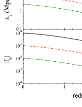
which implies that the gravitational constant is enhanced by . This leads to the scale-dependent enhancement of the linear growth rate. This linearisation around the cosmological background fails when becomes larger compared with the background field , . This happens in the dense region because is driven by the matter perturbations . In these dense regions, the curvature is large and Eq. (16) ensures that is suppressed and GR is recovered, realising the Chameleon mechanism. In Fig. 1, we plot the time evolution of the Compton wavelength and the background field with and , which is useful to understand the recovery of GR in our simulations.
III The -body Simulations
In the model of Hu:2007nk , the fifth force due to the propagation of is suppressed by many orders of magnitudes than gravity only in very dense regions, while in less dense regions it has similar strength as gravity. Such a dramatic change of the amplitude of the fifth force across space indicates that Eq. (6) should be highly nonlinear, which the readers can convince themselves by appreciating the nonlinearity of [cf. Eq. (14)]. Consequently treatments involving linearisation fails to make correct predictions, and -body simulations which explicitly solve the nonlinear equation for are needed.
In a series of papers Oyaizu:2008sr ; Oyaizu:2008tb ; Schmidt:2008tn , Oyaizu et al. pioneered in this direction, by solving Eq. (6) on a regular mesh to compute the total force on particles. Their results show some interesting and cosmologically testable predictions of the gravity. However, the resolution of their simulations was limited by their regular mesh. Here, we perform similar simulations, but with an adaptive grid which self-refines in the high density regions. This technique has been applied previously in Li:2009sy ; Li:2010mq ; Li:2010nc and works well.
As we are interested in how well the Chameleon mechanism actually works, besides the full simulations, we also perform some non-Chameleon runs with the Chameleon effect artificially suppressed (see below). For clarity we shall refer to these two classes of simulations respectively as full and non-Chameleon simulations.
III.1 Outline of the Simulation Algorithm
We have modified the publicly available -body simulation code MLAPM Knebe:2001 , which is a self-adaptive particle mesh code, for our -body simulations. It has two sets of meshes: the first mesh includes a series of increasingly refined regular meshes covering the whole cubic simulation box, with respectively cells on each side, where is the size of the domain grid, which is the most refined of these regular meshes. This set of meshes are needed to solve the Poisson equation using multigrid method or fast Fourier transform (for the latter only the domain grid is necessary). When the particle density in a cell exceeds a predefined threshold, the cell is further refined into eight equally sized cubic cells; the refinement is done on a cell-by-cell basis and the resulted refinement could have arbitrary shape which matches the true equal-density contours of the matter distribution. This second set of meshes are used to solve the Poisson equation using a linear Gauss-Seidel relaxation.
Our core change to the MLAPM code is the addition of the routines which solve Eq. (6), which is similar to that in Li:2010mq ; Li:2010nc . These include:
-
1.
We have added a solver for , based on Eq. (6), which uses a nonlinear Gauss-Seidel relaxation iteration and the same convergence criterion as the default Poisson solver of MLAPM. It adopts a V-cycle instead of the default self-adaptive scheme in arranging the Gauss-Seidel iterations, because the latter is found to be plagued by the problem of oscillations between adjacent multigrid levels, and the convergence is too slow.
-
2.
The value of solved from the above step is used to complete the computation of the source term for the Poisson equation Eq. (7), which is solved using a fast Fourier transform on the regular domain grids and Gauss-Seidel relaxation on the irregular refinements.
-
3.
The value of solved from the above step is used to compute the total force on the particles by a finite difference, and then the particles are displaced and accelerated as in usual -body simulations, according to
(21) (22)
where a subscript c denotes code unit. More details about the code could be found in Knebe:2001 ; Li:2010nc .
III.2 -body Equations in Code Units
To implement Eqs. (6, 7) into our numerical code, we have to rewrite them using code units, which are given by
| (23) |
where is the size of the simulation box and km/s/Mpc. We also need to choose a code unit for (or ), but this is done in different ways for the Chameleon and non-Chameleon simulations for convenience, and here we shall discuss them separately.
III.2.1 The Full Simulations
In our full simulations, the quantity in Eq. (6) is written in its exact form with
| (24) | |||||
| (25) |
where and are respectively the present fractional energy densities for matter and dark energy, and . With the aid of these, we can rewrite Eq. (6) using code units as
| (26) | |||||
Note that we will drop the subscript of for simplicity from now on.
In the simulations, spans a range of many orders of magnitude, from in the very dense regions to in the low density regions. Obviously, the above equation is very sensitive to numerical errors in the trial solution to , making it difficult to solve accurately. Furthermore, Eq. (24) indicates that would lead to unphysical (imaginary) , and if this happens by accident in the simulations due to the numerical errors (which is very likely because ) then the computation cannot carry on further. To solve these problems, we introduce a new variable (which is slightly different from the choice of Oyaizu:2008sr ). Then, typically , which does not vary much across the simulation box and no matter which value takes.
Replacing with , we can rewrite Eq. (26) as (after some rearrangement),
| (27) | |||||
Similarly, in terms of and using the code units, we can rewrite the Poisson equation as,
| (28) | |||||
III.2.2 The Non-Chameleon Simulations
As mentioned above, because the Chameleon effect is one of the most important features of our model, we also would like to see what happens if we artificially suppress it. Unlike Oyaizu:2008tb ; Schmidt:2008tn , in our simulations we achieve this by explicitly linearising the equation for without using the solution for given in Eq. (19). Since the Chameleon effect originates from the nonlinearity of , the linearisation will largely weaken it, justifying the name non-Chameleon simulations.
The linearisation is easily done by simply setting , which changes Eq. (6) to
| (29) |
In this case, we find it more convenient to choose as our variable, then using the relation
| (30) |
we can rearrange the above equation to obtain
| (31) | |||||
Note that after the linearisation the mass of the scalaron depends only on the background matter density; but if is chosen to be small enough (such that ) the mass can be very heavy, and thus the fifth force still gets suppressed, even though the suppression is not as strong as in the full simulations. Furthermore, the suppression of the fifth force in this case is universal and independent of the local matter density, again justifying its name – non-chameleon model.
Similarly, the modified Poisson equation appears to be
| (32) | |||||
III.3 Code Tests
As the major modification to the MLAPM code is for the solver, we have to check carefully whether it works correctly. For this purpose we have solved Eq. (27) around a point-like mass Oyaizu:2008sr and compared the result with the analytic solution; we find that the numerical and analytic solutions agree as well as in Oyaizu:2008sr (Fig. 2 there). To avoid repetition we shall not display the results here.
Other, indirect, tests of our code include comparing the predicted matter power spectrum to the linear perturbation results to see whether they agree on large scales. We shall discuss these in turn as the paper unfolds.
III.4 Simulation Details
| Box size (Mpc/h) | |||
| 10 | 10 | 10 | |
| 128 | 128 | 128 | |
| (h/Mpc) | |||
| (h/Mpc) | 5.5 | 11.0 | 22.0 |
| Refinement levels | 8 | 9 | 10 |
| Force resolution (Kpc/h) | 12 | 23 | 94 |
| Mass resolution (/h) | 13.3 | 1.75 | 0.21 |
We choose to run our simulations in a cosmology that is consistent with the WMAP observations. Specifically, we parametrise the universe in the form of
| (33) |
The symbols and denote the subsets of cosmological and parameters, respectively.
| (34) |
where and denote the physical energy density for baryons and cold dark matter respectively, is the curvature, is the Hubble constant today, stands for the index of the primordial power spectrum at a pivot scale of Mpc-1, and measures the amplitude of the (linear) power spectrum on the scale of Mpc/h.
| (35) |
Here and specify a model as described in Sec. II. We set the cosmological parameters as , while for the parameters, we fix and simulate for three models with . We also run the standard GR model () for the purpose of comparison. For each model, we also run the simulation without the Chameleon mechanism using the same initial condition and background evolution. Since we will refer to these simulations frequently later in the text, we assign them abbreviations to lighten the notations, as listed below,
-
•
F4 = Full simulation with ;
-
•
F5 = Full simulation with ;
-
•
F6 = Full simulation with ;
-
•
N4 = non-Chameleon simulation with ;
-
•
N5 = non-Chameleon simulation with ;
-
•
N6 = non-Chameleon simulation with ;
-
•
GR = Simulation for a CDM model in GR.
For each model listed above, we run 10 simulations with 10 different initial conditions (ICs), which we call 10 ‘realisations’, to reduce the sample variance. To extend the range of scales, we run these simulations in 3 difference boxes with size and Mpc/h. The technical details are summarised in Table 1. We generate the ICs using Grafic, an IC generator included in the COSMICS package Bertschinger:1995er , at redshift in GR, and then evolve the system using our modified version of MLAPM for , as well as using the default MLAPM for GR simulations.
III.5 Data Analysis
Data analysis is of great significance for the simulation. In this section, we will detail our pipeline to obtain the snapshots, matter power spectra, mass function and the density and scalar field profiles out from the raw simulation output.
III.5.1 Snapshots
Visualisations of the simulation result is helpful to understand the physics in an intuitive way. For this purpose, we will show the 2-D snapshots for the distribution of overdensity , the perturbation of the scalar field and gravitational potential . For the visualisation, we output the data for ln, and on a grid from our simulation, and project the 3-D volume onto a 2-D plane to make image snapshots. The resolution we use here is much lower than that we use for calculation in the code, but it is sufficient for the purpose of visualisation.
III.5.2 Binning, Average and Variance
We will present our simulation results (power spectra, mass function and profiles) in terms of data bins along with error bars. Suppose our observable is called which is a function of , and we have raw samples measured from simulation for in some range of that we are interested in, then we take an average of over 10 realisations first, make logarithmic bins in , and then calculate the mean value and error bar for the th bin via,
| (36) |
where is the total number of raw samples falling into the th bin.
III.5.3 Matter Power Spectrum
The matter power spectrum is an important statistical measure of the matter clustering on different scales in Fourier space. We measure the matter power spectrum using a tool called POWMES Colombi:2008dw . POWMES estimates the Fourier modes of a particle distribution based on a Taylor expansion of the trigonometric functions, and it is able to accurately determine and correct for the biases induced by the discreteness and by the truncation of the Taylor expansion. Also, the aliasing effect is safely negligible if the order of Taylor expansion , which we chose to use. One could even accurately measure up to the scale of (Box size) with the ‘folding’ operation, which we adopted in our analysis.
We firstly measure the power spectrum for GR simulations using POWMES, and use as the observable . Then we utilise Eq. (36) to estimate the mean value and error bar for for each bin and compare it to the Halofit (Smith et al., Ref. Smith:2002dz ) prediction. Then we measure the power spectra for full and non-Chameleon simulations, use the relatively difference
| (37) |
as the observable and similarly use Eq. (36) to get estimates of .
III.5.4 Halo Mass Function
We use the MHF tool Gill:2004km (the Halo-finder for MLAPM) to resolve halos in our simulation. The halo-finding algorithm we use is similar to that in Ref. Schmidt:2008tn – we assign the particles to the grids using a Triangular Shaped Cloud (TSC) interpolation, and count the particles within a sphere around the highest overdensity grid point. We increase the radius of the sphere until the overdensity reaches a threshold . This process can be repeated until all the halos are identified, and we only keep those that are made of at least particles for our analysis. In this paper we choose to be the virial overdensity in CDM model, . Thus the mass is defined by where is the radius when the overdensity reaches the threshold . depends on redshifts; at and at in our GR models. We use the same definition of the mass in simulations in order to make a fair comparison between gravity models and GR models. However, we should bear in mind that in gravity the virial overdensity is different from that in GR Schmidt:2008tn and a care must be taken when we compare the mass function in our simulations to observations.
In this work we use the definition of the halo mass function as the halo number density per logarithmic interval in the virial mass in GR, i.e.,
| (38) |
This definition is different from Ref. Schmidt:2008tn where they use to define the mass. Thus a direct comparison is not possible without rescaling the mass.
Since the halos in and GR simulations have different number and mass in general 444The number and mass of the halos are in general different even for the same gravity model for different realisations., and we are interested in the relative difference of the mass function in model with respect to that in GR, we need to make sure that we are comparing the same quantity in different gravity models. Therefore, for the simulations with the same box size, we find the overlapping halo mass range for full , non-Chameleon and GR simulations for all the 10 realisations, and make logarithmic bins in mass in this range. Then we count the number of halos falling into each mass bin for and GR cases respectively, and calculate the relative difference for each bin for every realisation. Finally we average over 10 realisations to calculate the mean value and variance for each mass bin.
III.5.5 Halo Profile
We modified MHF to analyse the profile of the perturbation of the scalar field , and the gravitational potential as well as the overdensity as a function of the rescaled virilised halo radius . To see the relative difference of the density profile with respect to that in GR, we have to identify the same halos in the full, non-Chameleon and GR simulations for each realisation. Since more halos are produced generally in models, we start from the GR halos in each realisation, and decide whether to include it for the analysis in the following steps,
-
1.
For the first realisation in GR, record the position and mass for the first halo, also the number of particles made up of this halo;
-
2.
For the same realisation for the 6 simulations [F4,F5,F6 and N4,N5,N6], search for the same halo as it in GR. If all the following conditions are satisfied,
-
(a)
The number of particles made up of this halo should be greater than ;
-
(b)
In all the 6 simulations, a halo with the similar position (absolute distance to the corresponding halo in GR smaller than 0.1% of the box size) and a similar mass (relative mass difference ) is found;
we assume it is the same halo as in GR simulations.
-
(a)
-
3.
Repeat the halo identification process so that all the halos with counterpart in are selected;
-
4.
For every selected halo, rescale to and linearly interpolate the overdensity to obtain for the same for different gravity models;
-
5.
Calculate the relative difference and feed into Eq. (36) to obtain the statistics for density profile.
It is interesting to test the working efficiency of Chameleon mechanism inside the halos, and this can be realised by comparing the profiles of to that of . If Chameleon does not work at all where the mass term of the scalar field can be ignored, i.e., , from Eqs. (6) and (7), we have
| (39) |
Therefore we define an efficiency parameter for the Chameleon mechanism as,
| (40) |
If then Chameleon hibernates, and if then it means Chameleon is very active. For the selected halos, we calculate for both full and non-Chameleon simulations and feed it into Eq. (36) to obtain the statistics for the profile of of the Chameleon mechanism.
IV Results
In this section, we will present our simulation results including the snapshots, matter power spectrum, the halo mass function and the profiles of the halo density and the efficiency parameter .
IV.1 Snapshots
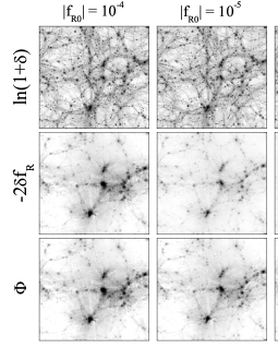
First, let us view the snapshots first to get some basic idea on the physics of our simulations. In Fig. 2, we show the snapshots for the density perturbation , the scalaron perturbation , and the gravitational potential taken from the full and non-Chameleon simulations for three values of . These snapshots are taken from one realisation with the box size Mpc/h at . The density plots show the familiar web-like structures, while the scalar field and potential have similar pattern, but are smoother. From the snapshots we can see that for the F4, F5, N4 and N5 simulations, and the Chameleon works very well for F6 cases () These are natural – the Chameleon mechanism works when and . Thus the F5 simulations are the critical case where the Chameleon mechanism is about to fail today. Note that in the N6 simulation we also find that is smaller than , because here the scalaron also has a heavy mass and a short Compton wavelength (though it is independent of local densities).
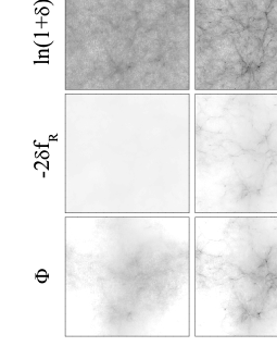
In Fig. 3, we show the same quantities for the F4 case at higher redshifts. Interestingly, we can see that the Chameleon does work very well at , and it hibernates at . This is because the background field is small at high redshifts (see Fig. 1) thus the condition for the Chameleon mechanism, , is easily satisfied.
IV.2 Matter Power Spectrum
In this section, we present the result for matter power spectrum in theory, in comparison with that in GR.
IV.2.1 Tests for GR simulations
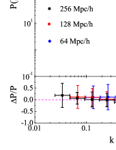
To start with, we test the accuracy of our GR simulations by comparing our results to the Halofit prediction Smith:2002dz . The result is shown in Fig. 4. As one can see, our Mpc/h simulation is very consistent with the Halofit prediction up to h/Mpc, namely, the relative difference is smaller than 10% on all scales. The Mpc/h simulation tends to underestimate the power at h/Mpc, which is due to the fact that we do not have enough particles to resolve small scales in a large box. The Mpc/h simulation shows much more power than that predicted by Halofit on scales h/Mpc. This does not necessarily mean that our simulation is not accurate on those scales, instead, the Halofit prediction has never been tested on such small scales, thus it might be inaccurate.
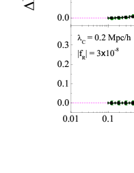
IV.2.2 Low-resolution tests for
After confirming that GR simulations are consistent with the Halofit predictions, we switch to the simulations. We did the full , Non-Chameleon and GR simulations in three different boxes with the size Mpc/h, and assemble them to extend the range of scale. Generally, the result is reliable up to the scale of , which is defined as,
| (41) |
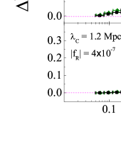
where is a factor determined by the adaptive nature of the code, and for the non-adaptive simulations, i.e., the pure particle-mesh (PM) simulations. The quantity is the half Nyquist scale, and and are the number of particles and the box size respectively (see Table 1 for the values we use in this work). Since for the first step we aim to reproduce the results in Ref. Schmidt:2008tn up to their resolution (half Nyquist scale), namely, h/Mpc, for a cross-check, we use the same -cutoff criterion as Ref. Schmidt:2008tn , namely, here we set . We will present our results on smaller scales, which is still reliable, in the next section. Given the spectra for different boxes, we take a volume-weighted average on the overlapped scales. In Fig. 5, we show the matter power spectra for both the full simulations and for the non-Chameleon cases at redshift . We took a ratio with respect to the GR power spectra with the same initial condition, and then averaged over ten different realisations to reduce the sample variance, as in Refs. Oyaizu:2008sr ; Oyaizu:2008tb ; Schmidt:2008tn .
As one can see, the growth is generally enhanced in gravity, and the peak value of the enhancement increases as . This is natural bacause, for large , e.g., , the Chameleon does not work, therefore the effective Newton’s constant is enhanced by below the Compton wavelength, resulting in a large enhancement of . For small , e.g., , Chameleon works very efficiently, which suppresses the structure growth back to that in GR locally, yielding a tiny enhancement of . The case for is critical – it is something between these two extreme cases, in which Chameleon works, but not as efficient as the case. Therefore the difference between full and the non-Chameleon simulations in this case is intermediate.
In Fig. 5, we overplotted the linear prediction, and the Halofit for gravity. The Halofit result is obtained by applying the Halofit fitting formula naively on the linear prediction for . Our simulations are consistent with linear predictions on large scales. The Halofit prediction overestimates the deviation from GR for smaller . This is because the Halofit uses only the information of linear power spectrum and fails to capture the effect of the Chameleon mechanism, which suppresses the deviation from GR. Note also the Halofit is calibrated in GR simulations. Thus once the deviation from GR becomes larger on smaller scales, we cannot trust the validity of the Halofit prediction. Our result is in prefect agreement with Refs. Oyaizu:2008tb ; Schmidt:2008tn .
IV.2.3 High-resolution results for
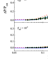
The self-adaptive nature of our code allows us to go beyond the half Nyquist scale, in other words, can be greater than . The realistic value of is largely determined by the maximum number of refinement triggered in the whole simulation process, which is for our simulations. To be conservative, we choose in all cases, and show the high-resolution result for power spectra in Figs. 6. As in Fig. 5, we show the relative difference of power spectra in with respect to that in GR at various redshifts.
Let us see the higher resolution result from Mpc/h simulations shown in Fig. 6 at and . Looking at the non-Chameleon result first, one could have the following observations,
-
1.
The ratio increases as one goes to small scales, and it goes down after reaching a peak at and for N4 and N5 cases;
-
2.
For the same model, the peak moves towards larger as one goes to higher redshift;
-
3.
The ratio monotonically increases with at for N4 and N5 cases and at all times for N6 cases.
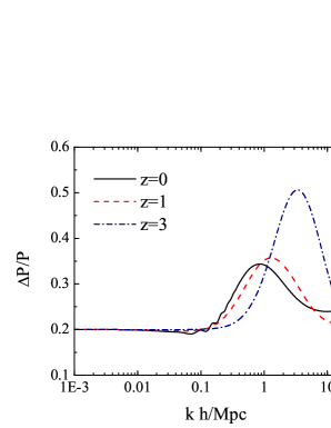
One could use GR as an example to understand these observations. It is true that GR is different from our non-Chameleon models, but the physical origin of these features are similar. In Fig. 7, we show the relative difference of matter power spectra in GR with with respect to that with at redshifts and . We use CAMB 555Available at http://camb.info to generate the linear power spectra, and use Halofit to account for the nonlinearities.
Interestingly, the pattern here is similar to what we saw just now – the ratio in GR shows a peak, and as increases, the peak becomes more pronounced, and it shifts to larger . This is due to the transition between the 2-halo term to the 1-halo term in the halo model description of the power spectrum (for a review see Cooray:2002dia ). If is higher, the non-linearity becomes important earlier and the transition from 1 to 2-halo term appears at smaller . Since the 2-halo term has a larger amplitude, this creates a peak in the ratio. As the transition wave number between 1 and 2-halo terms moves to smaller for smaller , the peak is shifted to smaller . The same thing happens in non-Chameleon simulations. In this case, the linear power has the -dependent enhancement. The transition from 1-halo to 2-halo term appears at high at in models but we do not see the peak as the -dependent enhancement of the linear power spectrum hides the enhancement due the 2-halo term. At , the transition appears at smaller where the linear enhancement is weak then we see the peak due to the transition from 1 to 2-halo term.
Having understood the non-Chameleon simulations results, now let us look at the full Chameleon simulations. At , we can see that the Chameleon mechanism works well even in the F4 case, and the deviation from GR is effectively suppressed. Once the Chameleon does not work well, e.g., at for F4, the full simulation result traces the non-Chameleon result as expected, with slightly lowered amplitude. Interestingly when the Chameleon mechanism has started to fail, e.g. at for F4 and at for F5, the power spectrum in full simulations has larger amplitudes than those in the non-Chameleon simulations on small scales. This implies that complicated dynamics is taking place when the Chameleon mechanism fails to work. We will come back to this issue later by studying the density profiles of halos. For the case where the Chameleon mechanism works very well, i.e., the F6 case, the full simulation result has much less amplitudes, implying that GR is successfully recovered.
IV.2.4 PPF fit
Hu and Sawicki proposed a fitting formula (PPF fit Hu07 ) for the matter power spectrum in modified gravity based on the assumption that the power spectrum resembles that in GR on small scales, which takes the form of,
| (42) |
where denotes the non-linear power spectrum in a CDM model with the same expansion history as that in the modified gravity models, and means the nonlinear power spectrum in modified gravity without the mechanism that recovers GR on small scales, i.e. the Chameleon mechanism. Therefore in our case, is exactly the power spectra for the non-Chameleon simulation, i.e., . measures the non-linearities and once the non-linearities are significant , the power spectrum approaches . Koyama et al. Koyama:2009me did a successful PPF fit and recovered the full simulation up to h/Mpc presented in Oyaizu:2008tb ; Schmidt:2008tn using Eq. (42) with given by
| (43) |
where is the linear power spectrum in .
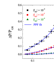
Since our simulation goes to much smaller scales than Oyaizu:2008tb ; Schmidt:2008tn , we study whether we can extend this fitting formula to smaller scales. To be conservative, we use the results from Mpc/h simulations to extend the formula up to h/Mpc (see Fig. 8). We generalise Eq. (43) by adding three more parameters and ,
| (44) |
Combining Eqs. (42) with (44), we fit up to h/Mpc, and the best-fit parameters are listed in Table 2. The best-fit power spectrum curves for models are overplotted with the simulation data in Fig. 9. As one can see, the agreement for F6 model is within one percent level even if we fixed and to zero. This implies that, if the Chameleon works, we can use the PPF formulae by varying and only. However, if the Chameleon fails, the power spectrum tends to go back to the non-Chameleon spectrum on small scales, so that we have to introduce additional parameters and to parametrise this behaviour. Once we include these parameters, we can fit the power spectrum in F4 and F5 models accurately. In the quasi non-linear regime h/Mpc, we can ignore the corrections described by and our results are roughly consistent with Koyama:2009me . The PPF fitting formula would be useful when we try to find fitting fomulae similar to Halofit in gravity models because the non-Chameleon simulations are far easier to run because of the linearity of the equation and the cosmological parameter dependence of the PPF parameters was found to be weak at least in the quasi non-linear regime.
| Redshift | ||||||
|---|---|---|---|---|---|---|
| fixed to | fixed to | |||||
| fixed to | fixed to | |||||
IV.3 Mass Function
IV.3.1 GR
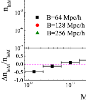
We test our mass function in GR firstly by comparing it to the theoretical predictions proposed by Sheth and Tormen Sheth:1999mn , and by Tinker et al.Tinker:2008ff . The comparison is shown in Fig. 10. We stack our results from different boxes to extend the mass range, and we see an agreement with theoretical predictions. It seems that our simulation underestimates the number of small halos (halos in the first bin) because of the lack of particles, but this problem can be alleviated to some extent when taking the ratio of the mass function of with respect to that in GR.
IV.3.2
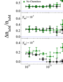
The result for the halo mass function is presented in Fig. 11. As one can see, our result at is consistent with that in Ref. Schmidt:2008tn (cf Fig. 2). Let us understand our result by looking at the non-Chameleon result first. In this case, the strength of gravity is enhanced by below the Compton wavelength , regardless of the value of . Meanwhile, increases with , making the enhancement on the mass function more pronounced for large models. This is what we see in Fig. 11. Also, at redshift , the enhancement for larger halos is more significant, while at redshift , smaller halos are more populated. This is because the stronger gravity in models create more small halos at high redshift and assemble them to make more large halos at low redshift compared with CDM models.
For the full simulations at , the number of massive halos is generally reduced compared to the non-Chameleon model predictions, because the suppression of the fifth force due to the Chameleon mechanism is stronger in high density regions, where massive halos most likely reside. For the case of , in which Chameleon does not work, the full and non-Chameleon results agree well, while for the case, the number of large halos is almost the same as the GR prediction due to the Chameleon effect. At redshift , the suppression starts from lower mass bins simply because Chameleon was working more efficiently at higher redshift.
IV.4 Halo Profile
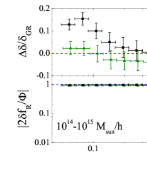
We show the halo profile for the overdensity and for at redshift and in Figs. 12 and 13 respectively. We show the results for the halos in three mass ranges: , and /h, taken from the and simulation boxes respectively.
A quick observation of the result is that on average, the profiles of the overdensity for gravity are similar to that in GR, namely, the relative difference is smaller than 20% in all cases. This is consistent with the analysis in Ref. Schmidt:2008tn . The complex patterns of the relative difference of and GR halo density profiles can be understood qualitatively as follows.
-
1.
For the F6 simulation, the Chameleon effect is very efficient throughout the cosmic history and so the fifth force has always been strongly suppressed, so that the predicted halo density profile should be very close to the GR result, which is what we see from Figs. 12 and 13 (the only exception is the case of low mass halos at , which is because these halos have lower density and so the Chameleon effect is weaker, especially at late times).
-
2.
For the N6 simulation, the fifth force is only weakly suppressed (especially at late times), and the central attractive potential towards the halo centre is stronger than in GR, which means that particles tend to fall towards the halo centres, producing higher density profiles than the latter.
-
3.
The N5 and N4 results follow the same pattern as N6, but are more complicated as in some cases the density profile can be even lower than in GR. This is perhaps because the central attractive potential is not the only thing affecting the halo density profile. As the fifth force is unsuppressed from early times, the particles are typically faster than they are in GR, and tend to escape the halo, flattening the density profile. Note that fifth force both deepens the central potential and speeds up the particles, and the latter is an accumulative effect, which makes it difficult to see which effect is dominating.
-
4.
The F4 simulation agrees with N4 simulation very well at late time, because Chameleon effect is insignificant. But at early times it produces higher density profile than N4, except for the small halos (for which Chameleon effect is again unimportant), which seems to indicate that the particles in the F4 halos are still relatively slow, because the fifth force has not become strong enough for long.
-
5.
The case of F5 is further complicated by the fact that is a critical point for our models. For the small halos, the fifth force has just become unsuppressed at , and we see that their density profiles are higher than N5 results for the same reason as above, while at the F5 and N5 simulations agree very well. For the medium-sized halos, at the fifth force is still strongly suppressed and their density profiles are lower than N5 results because the central attractive potential is weaker, while at the fifth force becomes unsuppressed and the density profiles are higher than N5 results again for the same reason as above. For the most massive halos, the fifth force is strongly suppressed even at present, and the halo density profiles are lower than in N5 for both and .
Therefore we see the following general evolution pattern when comparing the halo density profiles from F and N simulations: at early times the fifth force is strongly suppressed in F simulations, and so the central potential is weaker there, producing lower density profiles; then the fifth force becomes unsuppressed and the central potential becomes as strong as in N simulations, while the particles are still moving relatively slowly, producing higher density profiles. This happens at in F4 simulations and in F5 simulations. Finally the particles move fast due to the fifth force, and the density profiles approach the non-Chameleon results as is seen in F4 simulations at . The transition happens earlier for models with larger and for smaller halos (in both cases the fifth force becomes unsuppressed earlier). What we see in Figs. 12 and 13 are just different stages of the above evolution pattern.
This picture is consistent with the behaviour of the power spectrum shown in Fig 6. Once the Chameleon mechanism fails and the density profile becomes higher than those in N simulations, the power spectrum in F simulations tend to be higher on smaller scales (at in F4 simulations and at in F5 simulations). Then it approaches non-Chameleon results later (at in F4 simulations). We expect to see the same evolution pattern in F5 and F6 simulations if we would continue our simulations in the future.
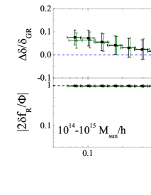
In Figs. 12 and 13 we have also shown the efficiency of the Chameleon effect. For the N4 and F4 simulations, we see that almost perfectly for both and , indicating that the Chameleon mechanism does not work for . Note that the agreement between N4 and F4 serves as an independent test of our code, as the treatments for these simulations are very different. For the N5 and F5 simulations, we see that is close to one for the small and medium-sized halos at both redshifts, while it is significantly less than for the massive halos, especially at , which are all as expected because the Chameleon effect is stronger in high density regions and at early times. is not perfectly equal to even at late times and in small halos, because there is a suppression of the fifth force and even in the linearised treatment above the Compton wavelength. In the N6 and F6 simulations, we see that for all halos and at all times, showing a strong Chameleon effect.
Interestingly, in the F simulations increases with the distance from the halo centre, while in N simulations the trend is just opposite (this is clearest in the F6/N6 simulations at ). The former is because the Chameleon effect gets weaker as one moves from the halo centre (highest density region) and so tends to ; the latter is because the value of is only affected by particles lying within the Compton wavelength from the considered position and as one moves from the halo centre more and more particles in the central region of the halo become unable to affect , while this does not happen to as gravity is a long-range force.
In summary, we find that the halo density profiles in the gravity model show complicate but interesting features, which could be understood qualitatively. We would like to study these in more details in future works, perhaps with the aid of even-higher-resolution simulations.
V Conclusion
Modified gravity scenario, especially the gravity, attracts more and more attention as an alternative to dark energy to explain the origin of the cosmic acceleration at low redshifts. Much efforts have been made to investigate the phenomenology of theories on linear scales Song:2007 ; Li:2007 ; Hu:2007nk ; Hu07 ; Pogosian:2007sw ; Zhao:2008bn . Unfortunately, the current observational data on linear scales, including weak lensing, Integrated Sachs-Wolfe (ISW) and cosmic microwave background (CMB), etc., can only weakly constrain gravity Song:2007da ; Giannantonio:2009gi ; Lombriser:2010mp . And even futuristic observations on linear scales can hardly prove, or falsify the scenario Zhao:2008bn .
On nonlinear scales, gravity can be much better tested by cosmological observations Schmidt:2009am ; Lombriser:2010mp because the scale dependent enhancement of the growth rate makes deviations from GR larger and larger on smaller scales. However, we should take into account the mechanism to recover GR that is necessary to evade the strong constraints in the solar system. In gravity models, this recovery of GR is accomplished by the Chameleon mechanism. In order to realise the Chameleon mechanism, the scalar mode in gravity should satisfy a highly non-linear evolution equation. In this work, we implement the Newton-Gauss-Seidel relaxation solver into the MLAPM code, an adaptive particle mesh simulation code, and obtain high resolution simulation results (up to h/Mpc for the matter power spectrum). We independently confirmed the results, including the power spectrum and halo statistics, presented in Refs. Oyaizu:2008tb and Schmidt:2008tn , and extended the resolution by a factor of .
Deviations from GR in the power spectrum are highly suppressed at early times when the Chameleon mechanism works very well. Later the Chameleon starts to fail once the background field becomes comparable to its fluctuations, . Then the power spectrum approaches the one in the case without the Chameleon mechanism. This transition happens at a higher redshift for a larger simply because the background field is larger for larger . We found an interesting behavior that the power spectrum in full Chameleon simulations has higher amplitude than the one in non-Chameleon simulations during this transition. We observed a similar behavior in the density profile. The density profile in full simulations becomes higher than the one in non-Chameleon simulations on small scales once the Chameleon has started to fail. Qualitatively, this is due to the fact that, once the Chameleon mechanism fails, the fifth force becomes unsuppressed and the central potential of halos becomes as strong as in the non-Chameleon simulations but the particles are moving still relatively slowly. Then dark matter particles are temporarily trapped at the central region of halos. Later particles velocities catch up and the density profile and the power spectrum approach those in non-Chameleon simulations. In order to confirm this picture, we would need higher resolution simulations and study the behavior of dark matter particles in halos carefully. We can also make the connection between the halo density profile and the power spectrum using the halo model approach. We leave the study of these issues in a separate paper.
We measured the profile of the scalaron field inside halos and studied the efficiency of the Chameleon mechanism As expected, we found that the Chameleon mechanism works better for heavier halos because the density is high in these halos. The halo mass function also shows the same tendency – the number of heavier halos approaches that in GR simulations if the Chameleon mechanism works as in the case. For the case, the Chameleon no longer works at , which results in more and more heavier halos compared with GR.
In conclusion, we studied the effect of the Chameleon mechanisms in details in our high resolution simulations. It was found that once the Chameleon mechanism stated to fail, the power spectrum and halo properties showed very interesting behaviours before they approach those in non-Chameleon simulations. For the power spectrum, we showed that this transition can be described by extending the Post-Parametrised-Friedmann (PPF) formalism that interpolates between the power spectrum in non-Chameleon models and GR models. This kind of fitting formulae will be useful when we confront our predictions to observations as it is far easier to run non-Chameleon simulations with different cosmological parameters. Our results indicate that is the critical case where the Chameleon mechanism fails to work today. It becomes significantly harder to detect deviations from GR once becomes smaller than . In this case, we need to look into the places where the Chameleon still fails to work, i.e. smaller halos. We leave a study of observational constraints on gravity using non-linear clustering such as weak lensing and cluster and voids abundance in a forthcoming paper.
Acknowledgements.
We thank Fabian Schmidt for enlightening discussions. GBZ thanks DAMTP of University of Cambridge for hospitality. GBZ and KK are supported by STFC grant ST/H002774/1. KK also acknowledges support from the European Research Council, the Leverhulme trust and RCUK. BL is supported by Queens’ College at University of Cambridge and STFC.Appendix A Discretisation of Equations
The last thing we are going to do before implementing the equations into the -body code is to discretise them, such that they fit to the philosophy of the numerical computations – solving the equations on meshes with finite grid sizes. This appendix displays the discretised equations, and again we discuss the Chameleon and non-Chameleon cases separately. We shall only write down the discrete equations for or , as those for as simple.
A.1 Full simulations
The full equation for , Eq. (27), contains the quantity . To discretise it, let us define , and assumed that the discretisation is performed on a grid with grid spacing . We shall require second order precision which is the same as the default Poisson solver in MLAPM, and then in one dimension can be written as
| (45) |
where a subscript means that the quantity is evaluated on the -th point. The generalisation to three dimensional case is straightforward.
The factor in makes this a standard variable coefficient problem. We need also discretise , and do it in this way (again for one dimension) Li:2009sy :
| (46) | |||||
in which . Generalising this to three dimensions, we have
| (47) | |||||
Then the discrete version of Eq. (27) is
| (48) |
in which
| (49) | |||||
Then the Newton-Gauss-Seidel iteration says that we can obtain a new (and usually more accurate) solution of , , using our knowledge about the old (and less acurate) solution as
| (50) |
The old solution will be replaced with the new one once the latter is ready, using a red-black Gauss-Seidel sweeping scheme. Note that
| (51) | |||||
In principle, if we start from some high redshift, then the initial guess of could be chosen as the background value because we expect that any perturbations should be small then. For subsequent time steps we can use either the solution at the last time step or some analytical approximated solution as the initial guess (for Chameleon simulations we find the latter more convenient while for non-Chameleon simulations it is just the opposite).
A.2 Non-Chameleon simulations
The discretisation of the equation Eq. (31) for the non-Chameleon simulations is much easier, and similarly to the above we have
| (52) |
in which
| (53) | |||||
with , and
| (54) |
References
- (1) S. Nojiri and S. D. Odintsov, ECONF C0602061, 06 (2006), hep-th/0601213.
- (2) K. Koyama, Gen. Rel. Grav. 40, 421 (2008), 0706.1557.
- (3) R. Durrer and R. Maartens, (2008), 0811.4132.
- (4) R. Durrer and R. Maartens, Gen. Rel. Grav. 40, 301 (2008), 0711.0077.
- (5) B. Jain, J. Khoury, Annals Phys. 325, 1479-1516 (2010). [arXiv:1004.3294 [astro-ph.CO]].
- (6) W. Hu and I. Sawicki, (2007), arXiv:0708.1190 [astro-ph].
- (7) J. Khoury and A. Weltman, Phys. Rev. D69, 044026 (2004), astro-ph/0309411.
- (8) T. P. Sotiriou and V. Faraoni, (2008), 0805.1726.
- (9) A. De Felice and S. Tsujikawa, Living Rev. Rel. 13, 3 (2010) [arXiv:1002.4928 [gr-qc]].
- (10) W. Hu and I. Sawicki, Phys. Rev. D76, 064004 (2007), 0705.1158.
- (11) A. A. Starobinsky, JETP Lett. 86, 157 (2007), 0706.2041.
- (12) S. A. Appleby and R. A. Battye, Phys. Lett. B654, 7 (2007), 0705.3199.
- (13) G. Cognola, E. Elizalde, S. Nojiri, S. D. Odintsov, L. Sebastiani and S. Zerbini, Phys. Rev. D 77, 046009 (2008) [arXiv:0712.4017 [hep-th]].
- (14) H. Oyaizu, Phys. Rev. D78, 123523 (2008), 0807.2449.
- (15) H. Oyaizu, M. Lima, and W. Hu, Phys. Rev. D78, 123524 (2008), 0807.2462.
- (16) F. Schmidt, M. V. Lima, H. Oyaizu, and W. Hu, (2008), 0812.0545.
- (17) R. E. Smith et al. [The Virgo Consortium Collaboration], Mon. Not. Roy. Astron. Soc. 341 (2003) 1311 [arXiv:astro-ph/0207664].
- (18) K. Koyama, A. Taruya and T. Hiramatsu, Phys. Rev. D 79 (2009) 123512 [arXiv:0902.0618 [astro-ph.CO]].
- (19) E. Beynon, D. J. Bacon and K. Koyama, Mon. Not. Roy. Astron. Soc. 403, 353 (2010) [arXiv:0910.1480 [astro-ph.CO]].
- (20) B. Li, D. F. Mota and J. D. Barrow, arXiv:1009.1400 [astro-ph.CO].
- (21) D. F. Mota and D. J. Shaw, Phys. Rev. D 75, 063501 (2006).
- (22) B. Li and J. D. Barrow, Phys. Rev. D 75, 084010 (2007) [arXiv:gr-qc/0701111].
- (23) Y. -S. Song, W. Hu and I. Sawicki, Phys. Rev. D 75, 044004 (2007) [arXiv:astro-ph/0610532].
- (24) B. Li and H. Zhao, Phys. Rev. D 80, 044027 (2009) [arXiv:0906.3880 [astro-ph.CO]].
- (25) B. Li and H. Zhao, Phys. Rev. D 81, 104047 (2009) arXiv:1001.3152 [astro-ph.CO].
- (26) B. Li and J. D. Barrow, arXiv:1005.4231 [astro-ph.CO].
- (27) A. Knebe, A. Green and J. Binney, Mon. Not. R. Astron. Soc., 325, 845 (2001).
- (28) E. Bertschinger, arXiv:astro-ph/9506070.
- (29) S. Colombi, A. H. Jaffe, D. Novikov and C. Pichon, arXiv:0811.0313 [astro-ph].
- (30) S. P. D. Gill, A. Knebe and B. K. Gibson, Mon. Not. Roy. Astron. Soc. 351 (2004) 399 [arXiv:astro-ph/0404258].
- (31) A. Cooray, R. K. Sheth, Phys. Rept. 372, 1-129 (2002). [astro-ph/0206508].
- (32) R. K. Sheth and G. Tormen, Mon. Not. Roy. Astron. Soc. 308 (1999) 119 [arXiv:astro-ph/9901122].
- (33) J. L. Tinker et al., Astrophys. J. 688 (2008) 709 [arXiv:0803.2706 [astro-ph]].
- (34) L. Pogosian and A. Silvestri, Phys. Rev. D 77 (2008) 023503 [Erratum-ibid. D 81 (2010) 049901] [arXiv:0709.0296 [astro-ph]].
- (35) G. B. Zhao, L. Pogosian, A. Silvestri and J. Zylberberg, Phys. Rev. D 79 (2009) 083513 [arXiv:0809.3791 [astro-ph]].
- (36) Y. S. Song, H. Peiris and W. Hu, Phys. Rev. D 76 (2007) 063517 [arXiv:0706.2399 [astro-ph]].
- (37) T. Giannantonio, M. Martinelli, A. Silvestri and A. Melchiorri, JCAP 1004 (2010) 030 [arXiv:0909.2045 [astro-ph.CO]].
- (38) L. Lombriser, A. Slosar, U. Seljak and W. Hu, arXiv:1003.3009 [astro-ph.CO].
- (39) F. Schmidt, A. Vikhlinin and W. Hu, Phys. Rev. D 80 (2009) 083505 [arXiv:0908.2457 [astro-ph.CO]].