Coupling optional Pólya trees and the two sample problem

Abstract

Testing and characterizing the difference between two data samples is of fundamental interest in statistics. Existing methods such as Kolmogorov-Smirnov and Cramer-von-Mises tests do not scale well as the dimensionality increases and provide no easy way to characterize the difference should it exist. In this work, we propose a theoretical framework for inference that addresses these challenges in the form of a prior for Bayesian nonparametric analysis. The new prior is constructed based on a random-partition-and-assignment procedure similar to the one that defines the standard optional Pólya tree distribution, but has the ability to generate multiple random distributions jointly. These random probability distributions are allowed to “couple”, that is to have the same conditional distribution, on subsets of the sample space. We show that this “coupling optional Pólya tree” prior provides a convenient and effective way for both the testing of two sample difference and the learning of the underlying structure of the difference. In addition, we discuss some practical issues in the computational implementation of this prior and provide several numerical examples to demonstrate its work.

1   Introduction

Two sample comparison is a fundamental problem in statistics. With two samples of data at hand, one often wants to answer the question—“Did these two samples come from the same underlying distribution?” In other words, one is interseted in testing the null hypothesis that the two data samples were generated from the same distribution. Moreover, in the presence of evidence for deviation between the two samples, one often hopes to learn the structure of such difference in order to understand, for example, what factors could have played a role in causing the difference. Hence two sample comparison is interesting both as a hypothesis testing problem and as a data mining problem. In this work, we consider the problem from both aspects, and develop a Bayesian nonparametric approach that can serve both the testing and the learning purposes.

Nonparametric hypothesis testing for two sample difference has a long history and rich literature, and many methods have been proposed. Some well-known examples include Wilcoxon test [11, p.243], Kolmogorov-Smirnov test [6, pp. 392–394] and Cramer-von-Mises test [1]. Recently, this problem has also been investigated from a Bayesian nonparametric perspective using a Pólya tree prior [10].

Despite the success of these existing testing methods for one-dimensional problems, two sample comparison in multi-dimensional spaces remains a challenging task. A basic idea for many existing methods is to estimate the two underlying distributions, and then use a distance metric to measure the dissimilarity between the two estimates. Tests such as Kolmogorov-Smirnov (K-S) and Cramer-von-Mises (CvM) fall into this category. However, reliably characterizing distributions in multi-dimensional problems, if computationally feasible at all, often requires a prohibitively large number of data points. With even just a moderate number of dimensions, the estimated distributional distance is often highly variable or biased. This “curse of dimensionality” demonstrates itself in the Bayesian setting as well. This is true even when the underlying difference is structurally very simple and can be accounted for by a relatively small number of dimensions in the space.

One general approach to dealing with the curse of dimensionality when characterizing distributions in a multi-dimensional space is to learn from the data a partition of the space that best reflects the underlying structure of the distribution(s). A good partition of the space overcomes the sparsity of the data by placing true neighbors together, and it reduces computational burden by allowing one to focus on the relevant blocks in the space. Hence it can be very helpful in multi-dimensional, and especially high-dimensional, settings to incorporate the learning of a representative partition of the space into the inference procedure. Wong and Ma [17] adopted this idea and introduced the optional Pólya tree (OPT) prior as such a method under the Bayesian nonparametric framework. Through optional stopping and randomized splitting of the sample space, a recursive partitioning procedure is incorporated into the parametrization of this prior, thereby allowing the data to suggest parsimonious divisions of the space. The OPT prior, like other existing Bayesian nonparametric priors, deals with only one data sample, but as we will demonstrate in this paper, similar ideas can be utilized for problems involving more than one sample as well.

Besides the difficulty in handling multidimensional problems, existing nonparametric methods for two sample comparison are also unsatisfactory in that they provide no easy way to learn the underlying structure of the difference should it exist. Tests such as K-S and CvM provide statistics with which to test for the existence of a difference, but does not allow one to characterize the difference—for example what variables are involved in the difference and how. One has to resort to methods such as logistic regression that rely on strong modelling assumptions to investigate such structure. Similarly, Bayes factors computed using nonparametric priors such as Dirichlet process mixture and the Pólya tree prior also shed no light on where the evidence for difference has arisen.

In this work, we introduce a new prior called “coupling optional Pólya tree” (co-OPT) designed for Bayesian nonparametric inference on the two sample problem. This new prior jointly generates two random distributions through a random-partitioning-and-assignment procedure similar to the one that gives rise to the OPT prior [17]. The co-OPT framework allows both hypothesis testing on the null hypothesis and posterior learning of the distributional difference in terms of a partition of the space that “best” reflects the difference structure. The ability to make posterior inference on a partition of the space also enhances the testing power for multi-dimensional problems.

This paper is organized as follows. In Section 2 we review the construction of the OPT distribution. In Section 3 we generalize the definition of the OPT distribution by replacing the “uniform base measure” (defined later) with a general absolutely continuous distribution, and show that this generalized prior can be used for investigating the goodness-of-fit of the data to the base distribution. In Section 4 we introduce the co-OPT prior and show how Bayesian inference can be carried out using this prior. In addition, we discuss the practical issues in implementing inference using this prior. In Section 5 we provide several numerical examples to illustrate inference on the two sample comparison problem using this prior and compare it to other methods. Then in Section 6 we present a method for inferring two common distributional distances, $L_{1}$ and Hellinger, between the two sample distributions using a co-OPT prior and provide two more numerical examples. Section 7 concludes with a few remarks.

We close this introduction with a few words on the recent development in the Bayesian nonparametric literature on related topics. In the past 15 years, several methods have been proposed for testing the one sample goodness-of-fit, in particular, for non-parametric alternatives against a parametric null. For some examples see [7, 5, 4, 3, 9, 13, 16]. As for two sample comparison, Holmes et. al. [10] introduced a way to compute the Bayes factor for testing the null through the marginal likelihood of the data with Pólya tree priors. Under the null, they model the two samples to have come from a single random measure distributed as a Pólya tree, while under the alternative from two separate Pólya tree distributions. In contrast, our new prior allows the two distributions to be generated jointly through one prior even when they are different. It is this joint generation that allows both the testing of the difference and the learning of the structure simultaneously. There are other approaches to joint modeling of multiple distributions in the Bayesian nonparametric literature. For example, one idea is to introduce dependence structure into Dirichlet processes [12]. For some notable examples see [14, 15, 8], among many others. Compared to these methods based on Dirichlet processes, our method, based on the optional Pólya tree, allows the resolution of the inference to be adaptive to the data structure and handles the sparsity in multidimensional settings using random partitioning [17]. Moreover, our method allows direct inference on the distributional difference without relying on inferring the two distributions per se, making it particularly suited for comparison across multiple samples. This point will be further discussed in Section 4.2 and illustrated in the examples given in Sections 5 and 6.

2   Optional Pólya trees and Bayesian inference

Wong and Ma [17] introduced the optional Pólya tree (OPT) distribution as an extension to the Pólya tree prior that allows optional stopping and randomized partitioning of the sample space $\Omega$, where $\Omega$ is either finite or a rectangle in an Euclidean space. One can think of this prior as a procedure for generating random probability measures on $\Omega$ that consists of two components—(1) random partitioning of the space and (2) random probability assignment into the parts of the space produced by the partitioning.

We first review how the OPT prior randomly partitions the space. Let $\mathcal{R}$ denote a partition rule function which, for any subset $A$ of $\Omega$, defines a number of ways to partition $A$ into a finite number of smaller sets. For example, for $\Omega=[0,1]\times[0,1]$, the (coordinate-wise) diadic split rule $\mathcal{R}$ is that $\mathcal{R}(A)$={ splitting $A$ in the middle of the range of one of the coordinates $x_{j}$, $j=1$ or 2} if $A$ is a non-empty rectangle and = $\emptyset$ otherwise. We call a rule function $\mathcal{R}$ finite if $\forall A\subset\Omega$, the number of possible ways to partition $A$, $M(A)$, as specified by $\mathcal{R}$, is finite. In the rest of the paper, we will only consider finite partition rules. Let $K^{j}(A)$ be the number of children specified by the $j$th way to partition $A$ under $\mathcal{R}(A)$, and let $A^{j}_{i}$ denote the $i$th child set of $A$ in that way of partitioning. That is, $A=\cup_{i}^{K^{j}(A)}A^{j}_{i}$ for $j=1,2,\ldots,M(A)$. We can write $\mathcal{R}(A)$ as

$$\mathcal{R}(A) =\{\{A^{1}_{1},A^{1}_{2},\ldots A^{1}_{K^{1}}\},\{A^{2}_{1},A^{2}_{2},\ldots,A^{2}_{K^{2}}\},\ldots\{A^{M}_{1},A^{M}_{2},\ldots A^{M}_{K^{M}}\}\}=\left\{\{A^{j}_{i}\}_{i=1}^{K^{j}}\right\}_{j=1}^{M},$$

where for simplicity we suppressed notation by writing $M$ for $M(A)$ and $K$ for $K(A)$.

A partition rule function $\mathcal{R}$ does not specify any particular partition on $\Omega$ but rather a collection of possible partitions over which one can draw random samples. The OPT prior samples from this collection of partitions in the following sequential way. Starting from the whole space $A=\Omega$. If $M(A)=0$, then $A$ is not divisible under $\mathcal{R}$ and we call $A$ an atom (set). In this case the partitioning of $A$ is completed. If $M(A)>0$, that is, $A$ is divisible, then a Bernoulli($\rho(A)$) random variable $S(A)$ is drawn. If $S(A)=1$, we stop partitioning $A$. Hence $S(A)$ is called the stopping variable for $A$, and $\rho(A)$ the stopping probability. If $S(A)=0$, $A$ is divided in the $J(A)$th of the $M(A)$ available ways for partitioning $A$ under $\mathcal{R}(A)$, where $J(A)$ is a random variable taking values $1,2,\ldots,M(A)$ with probabilities $\lambda_{1}(A),\lambda_{2}(A),\ldots,\lambda_{M(A)}(A)$ respectively, and $\sum_{j=1}^{M(A)}\lambda_{j}(A)=1$. $J(A)$ is hence called the (partition) selector variable, and $\bm{\lambda}(A)=(\lambda_{1}(A),\lambda_{2}(A),\ldots,\lambda_{M(A)}(A))$ the (partition) selector probabilities. If $J(A)=j$, we partition $A$ into $\{A^{j}_{1},A^{j}_{2},\ldots A^{j}_{K^{j}(A)}\}$, and then apply the same procedure to each of the children. In addition, if $A$ is reached from $\Omega$ after $k$ steps (or levels) of recursive partitioning, then we say that $A^{j}_{i}$ is reached after $k+1$ steps (or levels) of recursive partitioning. (To complete this inductive definition, we say that the space $\Omega$ is reached after 0 steps of recursive partitioning.) The recursive partitioning procedure naturally gives rise to a tree structure on the sample space. For this reason, we shall also refer to the sets $A$ that arise during the precedure as (tree) nodes.

The first question that naturally arises is whether this sequential procedure will eventually “stop” and produce a well defined partition on $\Omega$. Given that the stopping probability $\rho(A)>\delta$ for some $\delta$ and all $A$, this is indeed true in the following sense. If we let $\mu$ be the natural measure on $\Omega$—the Lebesgue measure if $\Omega$ is a rectangle in an Euclidean space or the counting measure if $\Omega$ is finite, then $\mu(T_{1}^{k})\rightarrow 0$ with probability 1, where $T_{1}^{k}$ is the part of $\Omega$ that is still not stopped after $k$ steps of recursive partitioning. In other words, the partitioning procedure will stop almost everywhere on $\Omega$.

The second component of the OPT prior is random probability assignment. The prior assigns probability mass into the randomly generated parts of the space in the following manner. Starting from $A=\Omega$, assign $Q(A)=1$ total probability to $A$. If $A$ is stopped or is an atom, then let the conditional distribution within $A$ be uniform. That is, $Q(\cdot|A)=u(\cdot|A)$, where $u$ denotes the uniform density (w.r.t.​ $\mu$) and this completes the probability assignment on $A$. If instead $A$ has children $\{A^{j}_{1},A^{j}_{2},\ldots A^{j}_{K^{j}(A)}\}$, (this occurs when $S(A)=0$ and $J(A)=j$,) a random vector $(\theta^{j}_{1}(A),\theta^{j}_{2}(A),\ldots,\theta^{j}_{K^{j}(A)}(A))$ on the $K^{j}(A)-1$ dimensional simplex is drawn from a Dirichlet($\alpha^{j}_{1}(A),\alpha^{j}_{2}(A),\ldots,\alpha^{j}_{K^{j}(A)}(A)$) distribution, and we assign to each child $A^{j}_{i}$ probability mass $Q(A^{j}_{i})=Q(A)\theta^{j}_{i}(A)$. We call $\bm{\theta}^{j}(A)=(\theta^{j}_{1}(A),\theta^{j}_{2}(A),\ldots,\theta^{j}_{K^{j}(A)}(A))$ the (probability) assignment vector, and $\bm{\alpha}^{j}(A)=(\alpha^{j}_{1}(A),\alpha^{j}_{2}(A),\ldots,\alpha^{j}_{K^{j}(A)}(A))$ the pseudo-count parameters. Then we go to the next level and assign probability mass within each of the children in the same way.

Theorem 1 in [17] shows that if $\rho(A)>\delta$ for some $\delta>0$ and all $A$, then with probability 1 this random partitioning and assignment procedure will give rise to a probability measure $Q$ on $\Omega$ that is absolutely continuous with respect to $\mu$. This random measure $Q$ is said to have an OPT distribution with (partition rule $\mathcal{R}$ and) parameters $\rho$, $\bm{\lambda}$ and $\bm{\alpha}$, which can be written as $OPT(\mathcal{R};\rho,\bm{\lambda},\bm{\alpha})$. In addition, Wong and Ma [17] also show that under mild conditions, this prior has large support—any $L_{1}$ neighborhood of an absolutely continuous distribution (w.r.t. $\mu$) on $\Omega$ has positive prior probability.

Two key features of the prior are demonstrated from the above constructive description. The first is self-similarity. If a set $A$ is reached as a node during the recursive partitioning procedure, then the continuing partitioning and assignment within $A$, which specifies the conditional distribution on $A$, is just an OPT procedure with $\Omega=A$. The second feature is the prior’s implicit hierarchical structure. To see this, we note that the random distribution that arises from such a prior is completely determined by the partition and assignment variables $S$, $J$, and $\bm{\theta}$, while the prior parameters $\rho$, $\bm{\lambda}$ and $\bm{\alpha}$ specify the distributions of these “middle” variables.

These two features allow one to write down a recursive formula for the likelihood under a random distribution arising from such a prior. To see this, first let $Q$ (with density $q$) be a distribution arising from an $OPT(\mathcal{R};\rho,\bm{\lambda},\bm{\alpha})$ distribution, and for $A\subset\Omega$, let $q(\cdot|A)$ be the conditional density on $A$. Let $S$, $J$, and $\bm{\theta}$ be the corresponding partition and assignment variables for $Q$ (or $q$). Suppose one has $n$ i.i.d. observations, $x_{1}$, $x_{2}$, …, $x_{n}$, on $\Omega$ from $q(\cdot|\Omega)$. Define

$$\bm{x}(A)=\{x_{1},x_{2},\ldots,x_{n}\}\cap A,$$

the observations falling in $A$, and $n(A)=|\bm{x}(A)|$, the number of observations in $A$. Then for any node $A$ reached in the recursive partitioning process determined by the $S$ and $J$ variables, the likelihood of observing $\bm{x}(A)$ conditional on $A$ is

$$q\left(\bm{x}(A)|A\right)=Su\left(\bm{x}(A)|A\right)+(1-S)\left(\prod_{i=1}^{K^{J}}\left(\theta_{i}^{J}\right)^{n(A_{i}^{J})}\right)\left(\prod_{i=1}^{K^{J}}q\left(\bm{x}\left(A_{i}^{J}\right)\big{|}A_{i}^{J}\right)\right),$$ (2.1)

where $u(\bm{x}(A)|A)=\frac{1}{\mu(A)^{n(A)}}$ is the likelihood under the uniform distribution on $A$, $S=S(A)$, $J=J(A)$, $K^{J}=K^{J(A)}(A)$, and $\theta_{i}^{J}=\theta_{i}^{J(A)}(A)$. (Note that for this formula to hold we need to define $q\left(\emptyset|A\right):=1$.) From now on we will always suppress the “(A)” notation for the random variables and the parameters where this adds no confusion. Similarly, we will use $q(\bm{x}|A)$ and $u(\bm{x}|A)$ to mean $q(\bm{x}(A)|A)$ and $u(\bm{x}(A)|A)$, respectively.

Integrating out $S$, $J$, and $\bm{\theta}$ in $\eqref{eq1}$, we get the corresponding recursive representation of the marginal likelihood

$$P(\bm{x}|A)=\rho u(\bm{x}|A)+(1-\rho)\sum_{j=1}^{M}\lambda_{j}\,\frac{D(\bm{n}^{j}+\bm{\alpha}^{j})}{D(\bm{\alpha}^{j})}\prod_{i=1}^{K^{j}}P\left(\bm{x}|A_{i}^{j}\right),$$ (2.2)

where $P(\bm{x}|A)=P(\bm{x}(A)|A)$, $\bm{n}^{j}=\bm{n}^{j}(A)=(n(A^{j}_{1}),n(A^{j}_{2}),\ldots,n(A^{j}_{K^{j}(A)}))$, and $D(\bm{t})=\Gamma(t_{1})\dots\Gamma(t_{k})/\Gamma(t_{1}+\dots+t_{k})$. Wong and Ma [17] provide terminal conditions so that (2.2) can be used to compute the marginal likelihood conditional on $A$, $P(\bm{x}|A)$, for all potential tree nodes $A$ determined by $\mathcal{R}$.

The final result we review in the section is the conjugacy of the OPT prior. More specifically, given the i.i.d. observations $\bm{x}$, the posterior distribution of $Q$ is again an OPT distribution with

1. Stopping probability: $\quad\rho(A|\bm{x})=\rho(A)u(\bm{x}|A)\big{/}P(\bm{x}|A)$

2. Selection probabilities:

   $$\lambda_{j}(A|\bm{x})\propto\lambda_{j}(A)\,\frac{D(\bm{n}^{j}+\bm{\alpha}^{j})}{D(\bm{\alpha}^{j})}\prod_{i=1}^{K^{j}}P\left(\bm{x}|A_{i}^{j}\right)\qquad\text{for $j=1,\ldots,M(A)$}$$

3. Probability assignment pseudo-counts: $\quad\alpha^{j}_{i}(A|\bm{x})=\alpha^{j}_{i}(A)+n(A^{j}_{i})$
   for $j=1,\ldots,M(A)$ and $i=1,2,\ldots,K^{j}(A)$

where again $A$ is any potential node determined by the partition rule function $\mathcal{R}$ on $\Omega$.

3   Optional Pólya trees and 1-sample “goodness-of-fit”

In the constructive procedure for an OPT distribution described above, whenever a node $A$ is stopped, the conditional distribution within it is generated from that of a baseline distribution, namely the uniform $u(\cdot|A)$. For this reason, we say that the collection of conditional uniform distributions, $\{u(\cdot|A):A\text{ is a potential node under }\mathcal{R}\}$, are the local base measures. With uniform local base measures, the stopping probability $\rho$ for a region $A$ represents the probability that the distribution is “flat” within $A$. Accordingly, the posterior OPT concentrates probability mass around partitions that best captures the “non-flatness” in the density of the data distribution. Such a partitioning criterion is most natural in the context of density estimation.

One can extend the original OPT construction by adopting different local base measures or stopping criteria for the nodes. More specifically, we can replace $u(\cdot|A)$ with any absolutely continuous measure $m^{A}(\cdot)$ on node $A$ in the probability assignment step. That is, when a tree node $A$ is stopped, we let the conditional distribution in $A$ be $m^{A}(\cdot)$. With this generalization, the recursive constructive procedure for the OPT distribution and the recipe for Bayesian inference described in the previous section still follow through.

One choice of the $m^{A}$ measures is of particular interest. Specifically, we can let $m^{A}(\cdot)=q_{0}(\cdot|A)$ for some absolutely continuous distribution $Q_{0}$ with density $q_{0}$ on $\Omega$. For this special case, we have the following definition.

Definition 1.

The random probability measure $Q$ that arises from the random-partitioning-and-assignment (RPAA) procedure described in the previous section, with $u$ replaced by $q_{0}$, the density (w.r.t.​ $\mu$) of an absolutely continuous distribution $Q_{0}$, is said to have an optional Pólya tree distribution on $\mathcal{R}$ with parameters $\bm{\lambda}$, $\bm{\alpha}$, $\rho$, and (global) base measure (or distribution) $Q_{0}$. We denote this distribution by $OPT(\mathcal{R};\bm{\lambda},\bm{\alpha},\rho;Q_{0})$.

The next theorem shows that by choosing an appropriate partitioning rule $\mathcal{R}$ and/or suitable pseudocount parameters $\bm{\alpha}$, one can enforce the random distribution $Q$ to “center around” the base measure $Q_{0}$.

Theorem 1.

If $Q\sim OPT(\mathcal{R};\rho,\bm{\lambda},\bm{\alpha};Q_{0})$, where $\delta<\rho(A)$ for some $\delta$ and all potential tree nodes $A$, then $\forall$ Borel set $B$,

$$EQ(B)=Q_{0}(B),$$

provided that for all $A$, $j=1,2,\ldots,M(A)$ and $i=1,2,\ldots,K^{j}(A)$, we have

$$\alpha^{j}_{i}(A)/\sum_{h=1}^{K^{j}(A)}\alpha^{j}_{h}(A)=Q_{0}(A^{j}_{i})/Q_{0}(A).$$

Proof.

See supplementary materials. ∎

Remark: If we have equal pseudocounts, that is, $\alpha^{j}_{1}(A)=\alpha^{j}_{2}(A)=\cdots=\alpha^{j}_{K^{j}(A)}(A)$ for all potential nodes $A$ and all $j$, then the condition for the theorem becomes $Q_{0}(A^{j}_{i})/Q_{0}(A)=1/K^{j}(A)$. Therefore one can choose a partition rule $\mathcal{R}$ on $\Omega$ based on the base measure to center the prior.

Bayesian inference using the OPT prior with a general base measure can be carried out just as before, provided we replace $u(\bm{x}|A)$ replaced by $q_{0}(\bm{x}|A)$ everywhere. An important fact is that a random distribution with this prior has positive probability to be exactly the same as the base distribution. Therefore, one can think of the inferential procedure for the OPT prior as a sequence of recursive comparison steps to the base measure. More specifically, the partitioning decision on each node $A$ is determined by comparing the conditional likelihood of the data within $A$ under $Q_{0}$ to the composite of $M(A)$ composite alternatives. The partition of each node $A$ stops when the observations in $A$ “fits” the structure of the base measure, and the posterior values of the partitioning variables capture the discrepancy, if any, between the data and the base. Consequently, this framework can be used to recursively test for 1-sample goodness-of-fit and to learn the structure of any potential “misfit”. For each node $A$, the posterior stopping probability is the probability that the data distribution coincides with the base distribution conditional on $A$. In particular, the posterior stopping probability for the whole space $\Omega$, $\rho(\Omega)$, measures how well the observed data fit the base overall. The posterior values of the other partitioning and pseudocount variables reflect where and how the data distribution differs from the base.

4   Coupling optional Pólya trees and two sample comparison

In this section we consider the case when two i.i.d. samples are observed and one is interested in testing and characterizing the potential difference between the underlying distributions. From now on, we let $Q_{1}$ and $Q_{2}$, with densities $q_{1}$ and $q_{2}$, be the two distributions from which the two samples have come from.

4.1   Coupling optional Pólya trees

A conceptually simple way to compare $Q_{1}$ and $Q_{2}$ is to proceed in two steps—first estimate the two distributions separately, and then use some distance metric to quantify the difference. For example, one can place an OPT prior on each of $Q_{1}$ and $Q_{2}$ and use the posteriors to estimate the densities [17]. (Other density estimators can also be used for this purpose.) With the density estimates available, one can then compute standard distance metrics such as $L_{1}$, and in turn use this as a statistic for testing the difference. (This approach provides no easy way to characterize how the two distributions are different.)

However, this two-step method is undesirable in multidimensional, and especially high-dimensional, settings. The main reason is that reliably estimating multidimensional distributions is a very difficult problem, and in fact often a much harder problem than comparing distributions. This difficulty in turn translates into either high variability or large bias in the distance estimates, and thus low statistical power. Using this approach, one is essentially making inference on the distributional difference indirectly, through the inference on a large number of parameters that characterize the two distributions per se but have little to do with their difference.

Following this reasoning, it is favorable to make direct inference on “parameters” that capture the distributional difference. But such direct inference requires (from a Bayesian perspective) that the two distributions be generated from a joint prior. This prior should be so designed that in the corresponding joint posterior, information regarding the distributional difference can be extracted directly. We next introduce such a prior.

Our proposed method for generating the two distributions $Q_{1}$ and $Q_{2}$ is again based on a procedure that randomly partitions the space $\Omega$ and assigns probability masses into the parts, similar to the one that defines the OPT prior. What differs from the procedure for the OPT is that we add in an extra random component—the conditional coupling of the two measures $Q_{1}$ and $Q_{2}$ within the tree nodes. We next explain this construction in detail. Starting from the whole space $A=\Omega$, we draw a random variable

$$C(A)\sim Bernoulli(\gamma(A)),$$

which we call the coupling variable. If $C(A)=1$, then we force $Q_{1}$ and $Q_{2}$ to be coupled conditional on $A$—that is, $Q_{1}(\cdot|A)=Q_{2}(\cdot|A)$—and we achieve this by generating a common conditional distribution from a stanford OPT on $A$. That is

$$Q_{1}(\cdot|A)=Q_{2}(\cdot|A)\sim OPT_{|A}(\mathcal{R};\rho,\bm{\lambda}^{b},\bm{\alpha}^{b}),$$

where the “b” superscript stands for “base”, and the “$|A$” notation should be understood as the restriction to $A$ of the partition rule $\mathcal{R}$, the stopping variables $\rho$, the partition selector variables $\bm{\lambda}^{b}$, and the assignment pseudo-count variables $\bm{\alpha}^{b}$. (For $A=\Omega$, there is no restriction.) If $C(A)=0$, then we draw a partition selector variable

$$J(A)\in\{1,2,\ldots,n\}\quad\text{with $P(J(A)=j)=\lambda^{j}(A).$}$$

If $J(A)=j$, then we partition $A$ under the $j$th way according to $\mathcal{R}(A)$. Then draw two independent assignment vectors

$$\bm{\theta}^{j}_{1}(A)=(\theta^{j}_{11}(A),\theta^{j}_{12}(A),\ldots,\theta^{j}_{1K^{j}(A)}(A)) \sim Dirichlet(\alpha^{j}_{11}(A),\alpha^{j}_{12}(A),\ldots,\alpha^{j}_{1K^{j}(A)}(A))$$

$$\bm{\theta}^{j}_{2}(A)=(\theta^{j}_{21}(A),\theta^{j}_{22}(A),\ldots,\theta^{j}_{2K^{j}(A)}(A)) \sim Dirichlet(\alpha^{j}_{21}(A),\alpha^{j}_{22}(A),\ldots,\alpha^{j}_{2K^{j}(A)}(A)),$$

and let

$$Q_{1}(A^{j}_{i})=Q_{1}(A)\theta^{j}_{1i}(A)\quad\text{and}\quad Q_{2}(A^{j}_{i})=Q_{2}(A)\theta^{j}_{2i}(A)$$

for each child $A^{j}_{i}$ of $A$. We call $\bm{\theta}^{j}_{1}(A)$ and $\bm{\theta}^{j}_{2}(A)$ the assignment vectors for $Q_{1}$ and $Q_{2}$ (in the uncoupled state). Then we go down one level and repeat the entire procedure for each $A^{j}_{i}$, starting from the drawing of the coupling variable.

Again, the first natural question to ask is whether this procedure will actually stop and give rise to two random probability measures $(Q_{1},Q_{2})$. The answer is positive under very mild conditions, and this is formalized in Theorem 2. The statement of the theorem uses the notion of “forced coupling”, which is similar to the idea of “forced stopping” used in the proof of Theorem 1 and which we describe next. Let $(Q_{1}^{(k)},Q_{2}^{(k)})$ denote the pair of random distributions arising from the above random-partitioning-and-assignment procedure with forced coupling after $k$-levels of recursive partitioning. That is, if after $k$ levels of partitioning a node $A$ is reached and the two measures are not coupled on it, then force them to couple on $A$ and generate $Q_{1}^{(k)}(\cdot|A)=Q_{2}^{(k)}(\cdot|A)$ from $OPT_{|A}(\mathcal{R};\rho,\bm{\lambda}^{b},\bm{\alpha}^{b})$. We do this for all such nodes to get $(Q_{1}^{(k)},Q_{2}^{(k)})$.

Theorem 2.

In the random-partitioning-and-assignment procedure for generating a pair of measures described above, if $\gamma(A),\rho(A)>\delta$ for some $\delta>0$ and all potential nodes $A$ defined by the partition rule $\mathcal{R}$, then with probability 1, $(Q_{1}^{(k)},Q_{2}^{(k)})$ converges to a pair of absolutely continuous (w.r.t. $\mu$) random probability measures $(Q_{1},Q_{2})$ in the following sense.

$$sup_{E\in\mathcal{B}}|Q_{1}^{(k)}(E)-Q_{1}(E)|+|Q_{2}^{(k)}(E)-Q_{2}(E)|\rightarrow 0,$$

where $\mathcal{B}$ is the collection of Borel sets.

Definition 2.

This pair of random probability measures ($Q_{1},Q_{2}$) is said to have a coupling optional Pólya tree (co-OPT) distribution with partition rule $\mathcal{R}$, coupling parameters $\bm{\lambda}$, $\bm{\alpha}_{1}$, $\bm{\alpha}_{2}$, $\gamma$, and base parameters $\bm{\lambda}^{b}$, $\bm{\alpha}^{b}$, $\rho$, and can be written as co-OPT$(\mathcal{R};\bm{\lambda},\bm{\alpha}_{1},\bm{\alpha}_{2},\gamma;\bm{\lambda}^{b},\bm{\alpha}^{b},\rho)$.

Proof of Theorem 2.

See supplementary materials. ∎

Similar to the OPT prior, the co-OPT distribution has large support under the $L_{1}$ metric. This is formulated in the following theorem.

Theorem 3.

Let $\Omega$ be a bounded rectangle in $\mathbb{R}^{p}$. Suppose that the condition of Theorem 2 holds along with the following two conditions:

• For any $\epsilon>0$, there exists a partition of the sample space allowed under $\mathcal{R}$, $\Omega=\cup_{i=1}^{I}A_{i}$, such that the diameter of each node $A_{i}$ is less then $\epsilon$.

• The coupling probabilities $\gamma(A)$, stopping probabilities $\rho(A)$, coupling selector probabilities $\lambda^{j}(A)$, base selection probabilities $\lambda^{b}_{j}(A)$, as well as the assignment probabilities $\alpha_{1i}^{j}(A)/(\sum_{l}\alpha_{1l}^{j}(A))$, $\alpha_{2i}^{j}(A)/(\sum_{l}\alpha_{2l}^{j}(A))$, and $\alpha_{i}^{bj}(A)/(\sum_{l}\alpha_{l}^{bj}(A))$ for all $i$, $j$ and all potential elementary regions are uniformly bounded away from $0$ and $1$.

Let $q_{1}=dQ_{1}/d\mu$ and $q_{2}=dQ_{2}/d\mu$, then for any two density functions $f_{1}$ and $f_{2}$, and any $\tau>0$, we have

$$P\left(\int|q_{1}(x)-f_{1}(x)|d\mu<\tau\text{ and }\int|q_{2}(x)-f_{2}(x)|d\mu<\tau\right)>0.$$

Proof.

See supplementary materials. ∎

4.2   Bayesian inference on the two sample problem using co-OPT prior

We next show that the co-OPT prior is conjugate and introduce the recipe for making inference on the two sample problem using this prior. Suppose $(Q_{1},Q_{2})$ is distributed as co-OPT$(\mathcal{R};\bm{\lambda},\bm{\alpha}_{1},\bm{\alpha}_{2},\gamma;\bm{\lambda}^{b},\bm{\alpha}^{b},\rho)$, and we observe two i.i.d.​ samples $\bm{x}_{1}=(x_{11},x_{12},\ldots,x_{1n_{1}})$ and $\bm{x}_{2}=(x_{21},x_{22},\ldots,x_{2n_{2}})$ from $Q_{1}$ and $Q_{2}$ respectively. For a node $A$ reached during the random partitioning steps in the generative procedure of $(Q_{1},Q_{2})$, let $\bm{x}_{1}(A)=\{x_{11},x_{12},\ldots,x_{1n_{1}}\}\cap A$ and $\bm{x}_{2}(A)=\{x_{21},x_{22},\ldots,x_{2n_{2}}\}\cap A$ be the observations from the two samples in $A$, and let $n_{1}(A)=|\bm{x}_{1}(A)|$ and $n_{2}(A)=|\bm{x}_{2}(A)|$ be the sample sizes in $A$. As before, we let $q_{1}$ and $q_{2}$ denote the densities of the two distributions and let $q^{A}_{0}$ denote the density of the random local base measure $Q^{A}_{0}$.

The likelihood of $\bm{x}_{1}(A)$ on $A$ under $q_{1}(\cdot|A)$ and that for $\bm{x}_{2}(A)$ under $q_{2}(\cdot|A)$ are

$$\left\{\begin{array}[]{ll}q_{1}(\bm{x}_{1}|A)=Cq^{A}_{0}(\bm{x}_{1})+(1-C)\prod_{i=1}^{K^{J}}(\theta^{J}_{1i})^{n_{1}(A^{J}_{i})}q_{1}(\bm{x}_{1}|A^{J}_{i})\\ \\ q_{2}(\bm{x}_{2}|A)=Cq^{A}_{0}(\bm{x}_{2})+(1-C)\prod_{i=1}^{K^{J}}(\theta^{J}_{2i})^{n_{2}(A^{J}_{i})}q_{2}(\bm{x}_{2}|A^{J}_{i})\end{array}\right.$$ (4.4)

where we have again suppressed the “(A)” notation for $C(A)$, $J(A)$, $K(A)^{J(A)}$, $\theta^{J(A)}_{1i}(A)$, $\theta^{J(A)}_{2i}(A)$, $\bm{x}_{1}(A)$ and $\bm{x}_{2}(A)$. The joint likelihood of observing $\bm{x}_{1}(A)$ and $\bm{x}_{2}(A)$ conditional on $A$ is

$$q_{1}(\bm{x}_{1}|A)q_{2}(\bm{x}_{2}|A)=Cq^{A}_{0}(\bm{x}_{1},\bm{x}_{2})+(1-C)\prod_{i=1}^{K^{J}}(\theta^{J}_{1i})^{n_{1}(A^{J}_{i})}(\theta^{J}_{2i})^{n_{2}(A^{J}_{i})}q_{1}(\bm{x}_{1}|A^{J}_{i})q_{2}(\bm{x}_{2}|A^{J}_{i}),$$ (4.5)

where $q^{A}_{0}(\bm{x}_{1},\bm{x}_{2})=q^{A}_{0}(\bm{x}_{1})q^{A}_{0}(\bm{x}_{2})$ is the standard OPT likelihood for the combined sample $\bm{x}(A)=(\bm{x}_{1}(A),\bm{x}_{2}(A))$ on $A$ given by (2.1). Integrating out $q^{A}_{0}$, $C$, $J$, $\bm{\theta}^{J}_{1}$ and $\bm{\theta}^{J}_{2}$ from (4.5), we get the conditional marginal likelihood

$$P(\bm{x}_{1},\bm{x}_{2}|A) =\gamma P_{0}(\bm{x}_{1},\bm{x}_{2}|A)+(1-\gamma)\sum_{j=1}^{M}\lambda_{j}\frac{D(\bm{n}_{1}^{j}+\bm{\alpha}_{1}^{j})D(\bm{n}_{2}^{j}+\bm{\alpha}_{2}^{j})}{D(\bm{\alpha}_{1}^{j})D(\bm{\alpha}_{2}^{j})}\prod_{i=1}^{K^{j}}P(\bm{x}_{1},\bm{x}_{2}|A^{j}_{i}),$$ (4.6)

where $\bm{n}_{h}^{j}=(n_{h}(A^{j}_{1}),n_{h}(A^{j}_{2}),\ldots,n_{h}(A^{j}_{K^{j}})$ and $\bm{\alpha}_{h}^{j}=(\alpha^{j}_{h1}(A),\alpha^{j}_{h2}(A),\ldots,\alpha^{j}_{hK^{j}}(A))$ for $h=1,2$, and $P_{0}(\bm{x}_{1},\bm{x}_{2}|A)$ is the conditional marginal likelihood of the combined sample under a standard OPT as given by (2.2). Equation (4.6) provides a recursive recipe for computing the marginal likelihood term $P(\bm{x}_{1},\bm{x}_{2}|A)$ for each potential tree node $A$. (Of course, for this recipe to be of use, one must also specify the terminal conditions for the recursion. We will discuss ways to specify such conditions in the next subsection.)

From (4.6) one can tell that the posterior distribution of $(Q_{1},Q_{2})$ is still a co-OPT distribution through the following reasoning. The first term on the RHS of $\eqref{eq:coOPT}$, $\gamma P_{0}(\bm{x}_{1},\bm{x}_{2}|A)$, is the probability (conditional on $A$ being a node reached in the partitioning) of the event

{$$Q_{1} Q_{2} A \bm{x}_{1}(A) \bm{x}_{2}(A)$$ and get coupled on , observe and }.

The second term, $(1-\gamma)\sum_{j=1}^{M}\lambda_{j}\frac{D(\bm{n}_{1}^{j}+\bm{\alpha}_{1}^{j})D(\bm{n}_{2}^{j}+\bm{\alpha}_{2}^{j})}{D(\bm{\alpha}_{1}^{j})D(\bm{\alpha}_{2}^{j})}\prod_{i=1}^{K^{j}}P(\bm{x}_{1},\bm{x}_{2}|A)$, is the probability of

{$$Q_{1} Q_{2} A \bm{x}_{1}(A) \bm{x}_{2}(A)$$ and are not coupled on , observe and }.

Each summand, $(1-\gamma)\lambda_{j}\frac{D(\bm{n}_{1}^{j}+\bm{\alpha}_{1}^{j})D(\bm{n}_{2}^{j}+\bm{\alpha}_{2}^{j})}{D(\bm{\alpha}_{1}^{j})D(\bm{\alpha}_{2}^{j})}\prod_{i=1}^{K^{j}}P(\bm{x}_{1},\bm{x}_{2}|A)$, is the probability of

{$$Q_{1} Q_{2} A A j \bm{x}_{1}(A) \bm{x}_{2}(A)$$ and not coupled on , divide in the th way, observe and }.

Finally, given that $C(A)=0$ and $J(A)=j$, the posterior distribution for $\bm{\theta}^{j}_{1}$ and $\bm{\theta}^{j}_{2}$ are Dirichlet$(\bm{n}_{1}^{j}+\bm{\alpha}_{1}^{j})$ and Dirichlet$(\bm{n}_{2}^{j}+\bm{\alpha}_{2}^{j})$, respectively. This reasoning, together with Theorem 3 in [17], shows that the co-OPT prior is conjugate, and simple applications of Bayes’ Theorem provide the formulae of the parameter values for the posterior. The results are summarized in the next theorem.

Theorem 4.

Suppose $\bm{x}_{1}=(x_{11},x_{12},\ldots,x_{1n_{1}})$ and $\bm{x}_{2}=(x_{21},x_{22},\ldots,x_{1n_{2}})$ are two independent i.i.d. samples from $Q_{1}$ and $Q_{2}$. Let $(Q_{1},Q_{2})$ have a co-OPT$(\mathcal{R};\bm{\lambda},\bm{\alpha}_{1},\bm{\alpha}_{2},\gamma;\bm{\lambda}^{b},\bm{\alpha}^{b},\rho)$ prior that satisfies the conditions in Theorem 2. Then the posterior distribution of $(Q_{1},Q_{2})$ is still a coupling optional Pólya tree with the following parameters.

1. Coupling probabilities: $\quad\gamma(A|\bm{x}_{1},\bm{x}_{2})=\gamma(A)P_{0}(\bm{x}_{1},\bm{x}_{2}|A)/P(\bm{x}_{1},\bm{x}_{2}|A).$

2. Partition selection probabilities:

   $$\lambda_{j}(A|\bm{x}_{1},\bm{x}_{2})\propto\lambda_{j}(A)\frac{D(\bm{n}_{1}^{j}+\bm{\alpha}_{1}^{j})D(\bm{n}_{2}^{j}+\bm{\alpha}_{2}^{j})}{D(\bm{\alpha}_{1}^{j})D(\bm{\alpha}_{2}^{j})}\prod_{i=1}^{K^{j}}P(\bm{x}_{1},\bm{x}_{2}|A),\quad j=1,2,\ldots,M(A).$$

3. Probability assignment pseudo-counts:

   $$\alpha^{j}_{1i}(A|\bm{x}_{1},\bm{x}_{2})=n_{1}(A^{j}_{i})+\alpha^{j}_{1i}(A)\quad\text{and}\quad\alpha^{j}_{2i}(A|\bm{x}_{1},\bm{x}_{2})=n_{2}(A^{j}_{i})+\alpha^{j}_{2i}(A),$$

   for $j=1,2,\ldots,M(A)$ and $i=1,2,\ldots,K^{j}(A)$.

4. Base stopping probabilities: $\quad\rho(A|\bm{x}_{1},\bm{x}_{2})=\rho(A)u(\bm{x}_{1},\bm{x}_{2}|A)/P_{0}(\bm{x}_{1},\bm{x}_{2}|A).$

5. Base selection probabilities:

   $$\lambda^{b}_{j}(A|\bm{x}_{1},\bm{x}_{2})\propto\lambda^{b}_{j}(A)\frac{D(\bm{n}_{1}^{j}+\bm{n}_{2}^{j}+\bm{\alpha}^{bj})}{D(\bm{\alpha}^{bj})}\prod_{i=1}^{K^{j}}P_{0}(\bm{x}_{1},\bm{x}_{2}|A),\quad j=1,2,\ldots,M(A).$$

6. Base assignment pseudo-counts: $\quad\alpha^{bj}_{i}(A|\bm{x}_{1},\bm{x}_{2})=n_{1}(A^{j}_{i})+n_{2}(A^{j}_{i})+\alpha^{bj}_{i}(A),$
   for $j=1,2,\ldots,M(A)$ and $i=1,2,\ldots,K^{j}(A)$.

Two remarks: (1) All of the posterior parameter values can be computed exactly using the above formulae, without the need of any Monte Carlo procedure. (2) The posterior coupling parameters contain information about the difference between the two underlying distributions $Q_{1}$ and $Q_{2}$, while the posterior base parameters contain information regarding the underlying structure of the two measures. This naturally suggests that if one is only interested in two sample comparison, one should only need the posterior distribution of the coupling variables, and not those of the base variables. This will become clear in Sections 5 and 6 where we give several numerical examples.

4.3   Terminal conditions

As mentioned earlier, we need to specify the terminal conditions for the recursion used to compute $P(\bm{x}_{1},\bm{x}_{2}|A)$. Depending on the nature of $\Omega$ and the prior specification, the recursion formula (4.6) can terminate in several ways as demonstrated in the following two examples.

Example 1 ($2^{p}$ contingency table).

Let $\Omega=\{1,2\}\times\{1,2\}\times\dots\times\{1,2\}$. For any rectangle $A$ in the table—a set of the form $A_{1}\times A_{2}\times\dots A_{p}$ with $A_{1}$, $A_{2}$, …, $A_{p}$ being non-empty subsets of $\{1,2\}$—let $k_{1},k_{2},\ldots,k_{M(A)}$ be the “intact” dimensions of $A$, that is $A_{k_{j}}=\{1,2\}$ for $j=1,2,\ldots,M(A)$. Let $\mathcal{R}$ be the diadic splitting rule that allows $A$ to be divided into two halves on each intact dimension $j$. In our earlier notation, $\mathcal{R}(A)=\left\{\{A^{j}_{1},A^{j}_{2}\}_{j=1}^{M(A)}\right\},$ where $A^{j}_{1}=A_{1}\times A_{2}\times\dots\times A_{k_{j}-1}\times\{1\}\times A_{k_{j}+1}\times\dots\times A_{p}$ and $A^{j}_{2}=A_{1}\times A_{2}\times\dots\times A_{k_{j}-1}\times\{2\}\times A_{k_{j}+1}\times\dots\times A_{p}$. Suppose two i.i.d.​ samples $\bm{x}_{1}$ and $\bm{x}_{2}$ are observed. Assume that $(Q_{1},Q_{2})$ has a co-OPT prior with the following prior parameter values for each rectangle $A$: $\lambda_{j}(A)=\lambda^{b}_{j}(A)=\tfrac{1}{M(A)}$, $\alpha_{i}^{j}(A)=\alpha_{i}^{bj}(A)\equiv\tfrac{1}{2}$ for $i=1,2$ and $j=1,2,\ldots,M(A)$, and finally $\gamma(A)\equiv\gamma_{0}$, $\rho(A)\equiv\rho_{0}$, where $\gamma_{0}$ and $\rho_{0}$ are constants in $(0,1)$.

In this example, there are three types of terminal nodes for $P_{0}(\bm{x}_{1},\bm{x}_{2}|A)$ and they are given in Example 3 of [17]. By a similar reasoning, there are also three types of terminal nodes for $P(\bm{x}_{1},\bm{x}_{2}|A)$.

1. If $A$ contains no data point from either sample, $P(\bm{x}_{1},\bm{x}_{2}|A)=1$.

2. If $A$ is a single table cell containing any number observations, $P(\bm{x}_{1},\bm{x}_{2}|A)=1$.

3. $A$ contains a single observation (from either sample). In this case, $P(\bm{x}_{1},\bm{x}_{2}|A)=2^{-M(A)}=1/\mu(A)$. To see this, first we let $t_{M(A)}=P(\bm{x}_{1},\bm{x}_{2}|A).$ By Example 3 in [17], we have $P_{0}(\bm{x}_{1},\bm{x}_{2}|A)=2^{-M(A)}.$ Hence we have

   $$t_{M(A)} =\gamma_{0}2^{-M(A)}+(1-\gamma_{0})\left(\dfrac{1}{M(A)}\sum_{j=1}^{M}\frac{B\left(\tfrac{3}{2},\tfrac{1}{2}\right)}{B\left(\tfrac{1}{2},\tfrac{1}{2}\right)}\right)\cdot t_{M(A)-1}$$

   $$=\gamma_{0}2^{-M(A)}+(1-\gamma_{0})\tfrac{1}{2}t_{M(A)-1}$$

   $$=\gamma_{0}2^{-M(A)}\,\frac{\left(1-(1-\gamma_{0})^{M(A)}\right)}{1-(1-\gamma_{0})}+\left(\frac{1-\gamma_{0}}{2}\right)^{M(A)}$$

   $$=2^{-M(A)}=1/\mu(A).$$

Example 2 (Rectangle in $\mathbb{R}^{p}$).

Let $\Omega=I_{1}\times I_{2}\times\ldots\times I_{p}$ be a bounded rectangle in $\mathbb{R}^{p}$. Let $\mathcal{R}$ be the diadic partition rule such that for any rectangle $A$ of the form $A_{1}\times A_{2}\times\dots A_{p}$ with $A_{1}$, $A_{2}$, …, $A_{p}$ being non-empty subintervals of $I_{1},I_{2},\ldots,I_{p}$ respectively, $A$ can be divided in half in any of the $p$ dimensions. Again, let $\bm{x}_{1}$ and $\bm{x}_{2}$ be the two samples, and let $(Q_{1},Q_{2})$ have a co-OPT prior with the following parameters: $\lambda_{j}(A)=\lambda^{b}_{j}(A)\equiv\tfrac{1}{p}$, $\alpha_{i}^{j}(A)=\alpha_{i}^{bj}(A)\equiv\tfrac{1}{2}$, $\gamma(A)\equiv\gamma_{0}$ and $\rho(A)\equiv\rho_{0}$, for all $A$, $i=1,2$, and $j=1,2,\ldots,M(A)$.

In this case there are two types of terminal nodes for $P(\bm{x}_{1},\bm{x}_{2}|A)$.

1. $A$ contains no observations. In this case, $P(\bm{x}_{1},\bm{x}_{2}|A)=1$.

2. $A$ contains a single observation (from either sample). Then $P(\bm{x}_{1},\bm{x}_{2}|A)=1/\mu(A)$. We skip the derivation of this as it is similar to that used for Case 3 in Example 1.

Note that in this example we have implicitly assumed that no observations, from either sample, can be identical. With the assumption that $Q_{1}$ and $Q_{2}$ are absolutely continuous w.r.t. the Lebesgue measure, the probability for any observations to be identical is 0. However this situation can occur in real data due to rounding. This possibility can be dealt with in our following discussion on technical termination of the recursion.

Other than the “theoretical” terminal nodes given in the previous two examples, in real applications it is often desirable to set a technical lower limit on the size of the nodes to be computed in order to save computation. For instance, in the $\mathbb{R}^{p}$ example, one can impose that all nodes smaller than 1/1000 of the space $\Omega$ be stopped and coupled. That is to let $\gamma(A)=\rho(A)=1$ by design for all small enough $A$. The appropriate cutoff threshold of the node size depends on the nature of the data, but typically there is a wide range of values that work well. For most problems such a technical constraint should hardly have any impact on the posterior parameter values for large nodes. It is worth emphasizing that for real-valued data, which are almost always discretized (due to rounding), such a constraint actually becomes useful also in preventing numerical anomalies. In such cases, a general rule of thumb is that one should always adopt a cutoff size larger than the rounding unit relative to the length of the corresponding boundary of the space.

5   Numerical examples on two sample comparison

We next provide three numerical examples, Examples 3 through 4, to demonstrate inference on the two sample problem using the co-OPT prior. In these examples, the posterior coupling probability of $\Omega$ serves as a statistic for testing whether the two samples have come from the same distribution, which we will refer to as the co-OPT statistic. In each example we compare our method to one or more other existing approaches, and in Example 4 we show how the posterior values of the coupling variables can be used to learn the underlying structure of the discrepancy between the two samples.

For all these examples, we set the prior parameter values in the fashion of Examples 1 and 2, with $\gamma_{0}=\rho_{0}=0.5$. In Examples 3 and 4, whenever the underlying distributions have unbounded support, we simply use the range of the data points in each dimension to define the rectangle $\Omega$. (As a referee pointed out, an alternative to using this data dependent support is to transform each unbounded dimension through a measurable map such as a cumulative distribution function. The choice of such maps will influence the underlying inference. Although we do not investigate this relation in the current work, it is certainly interesting and deserve further studies in future works.) Also, in these three examples we use 1/1000 as the size cutoff for “technical” terminal nodes as discussed in the previous section.

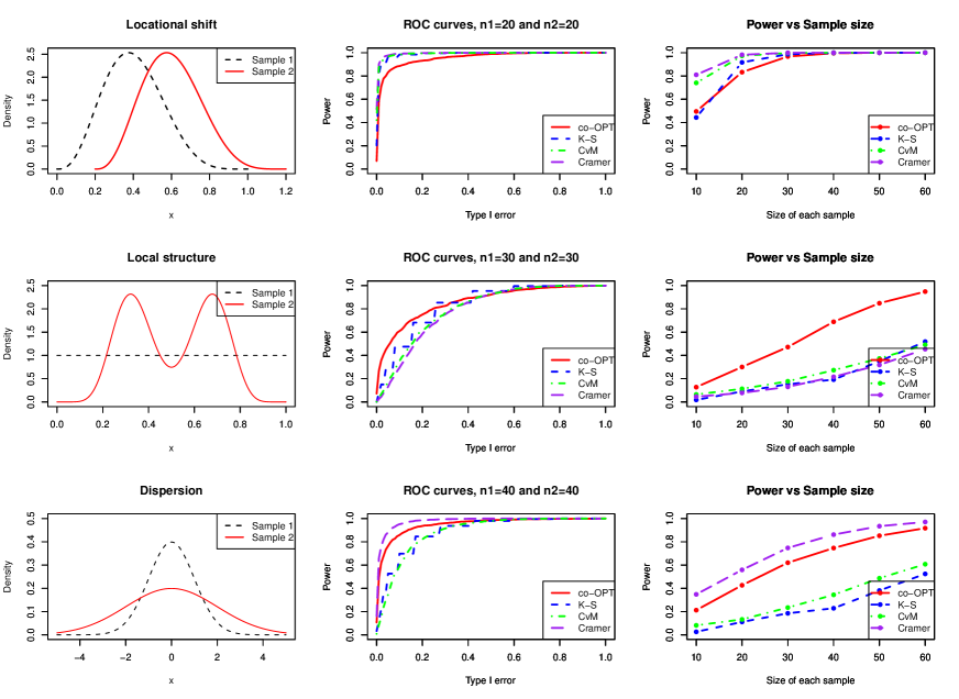
Example 3 (Two sample problem in $\mathbb{R}$).

We simulate the control and case samples under the following three scenarios.

1. Locational shift: Sample 1 $\sim$ Beta(4,6) and Sample 2 $\sim$ 0.2 + Beta(4,6) with sample sizes $n_{1}=n_{2}=20$.

2. Local structure: Sample 1 $\sim$ Uniform[0,1] and Sample 2 $\sim$ 0.5 Beta(20,10) + 0.5 Beta(10,20) with $n_{1}=n_{2}=30$.

3. Dispersion difference: Sample 1 $\sim$ N(0,1) and Sample 2 $\sim$ N(0,4) with $n_{1}=n_{2}=40$.

We place a co-OPT prior on $(Q_{1},Q_{2})$ as described in Example 2. (Because here there is only one dimension, there is no choice of ways to split.) We compare the ROC curves of four different statistics for testing the null hypothesis that the two samples have come from the same distribution—namely the Kolmogorov-Smirnov (K-S) statistic [6, pp. 392–394], Cramer-von-Mises (CvM) statistic [1], Cramer-test statistic [2], and our co-OPT statistic. The results are presented in the middle column of 1. In addition, we also investigate the power of each statistic at the 5% level under various sample sizes, ranging from 10 data points per sample to 60 per sample. (See the right column of 1.) Our co-OPT statistic behaves worse than the other three tests under the first scenario when there is a simple locational shift, better than the other tests for the second scenario, slightly worse than the Cramer test but better than the K-S and CvM tests under the last scenario.

Figure 1: Two simulated samples on $\mathbb{R}$ under three scenarios (rows) given in Example 3. Left panel: Density functions for the two samples. Middle panel: ROC curves for four test statistics. Right panel: Power vs. sample size—power (at the 5% level) is estimated from simulation under equal sample size (horizontal axis) of the case group and the control group.

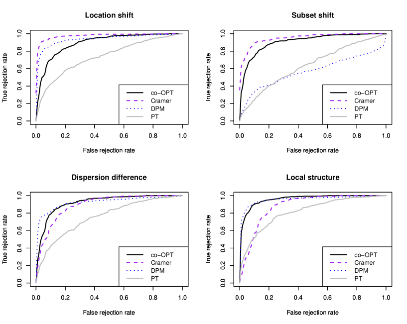
Example 4 (Two sample problem in $\mathbb{R}^{2}$).

We simulate two samples under four scenarios.

1. Locational shift ($n_{0}=n_{1}=50$):

   Sample 1 $\sim BN\Biggl{(}\begin{pmatrix}1\\ 0\end{pmatrix},\begin{pmatrix}2^{2}&0\\ 0&2^{2}\\ \end{pmatrix}\Biggr{)}$ and Sample 2 $\sim BN\Biggl{(}\begin{pmatrix}0\\ 1\end{pmatrix},\begin{pmatrix}2^{2}&0\\ 0&2^{2}\\ \end{pmatrix}\Biggr{)}$.

2. Subset shift ($n_{0}=n_{1}=100$):

   Sample 1 $\sim BN\Biggl{(}\begin{pmatrix}0\\ 0\end{pmatrix},\begin{pmatrix}0.3^{2}&0\\ 0&0.3^{2}\\ \end{pmatrix}\Biggr{)}$ and
   Sample 2 $\sim 0.8\times BN\Biggl{(}\begin{pmatrix}0\\ 0\end{pmatrix},\begin{pmatrix}0.3^{2}&0\\ 0&0.3^{2}\\ \end{pmatrix}\Biggr{)}+0.2\times BN\Biggl{(}\begin{pmatrix}0.5\\ 0.5\end{pmatrix},\begin{pmatrix}0.3^{2}&0\\ 0&0.3^{2}\\ \end{pmatrix}\Biggr{)}$.

3. Dispersion difference ($n_{0}=n_{1}=50$):

   Sample 1 $\sim BN\Biggl{(}\begin{pmatrix}0\\ 0\end{pmatrix},\begin{pmatrix}1&0\\ 0&1\\ \end{pmatrix}\Biggr{)}$ and Sample 2 $\sim BN\Biggl{(}\begin{pmatrix}0\\ 0\end{pmatrix},\begin{pmatrix}0.5^{2}&0\\ 0&0.5^{2}\\ \end{pmatrix}\Biggr{)}$.

4. Local structure ($n_{0}=n_{1}=50$):

   Sample 1 $\sim BN\Biggl{(}\begin{pmatrix}0\\ 0\end{pmatrix},\begin{pmatrix}1&0.5^{2}\\ 0.5^{2}&1\\ \end{pmatrix}\Biggr{)}$, and

   Sample 2 $\sim 0.5\times BN\Biggl{(}\begin{pmatrix}0.5\\ 0.5\end{pmatrix},\begin{pmatrix}0.4^{2}&0\\ 0&0.4^{2}\\ \end{pmatrix}\Biggr{)}+0.5\times BN\Biggl{(}\begin{pmatrix}-0.5\\ -0.5\end{pmatrix},\begin{pmatrix}0.4^{2}&0\\ 0&0.4^{2}\\ \end{pmatrix}\Biggr{)}$.

We compare four statistics that measure the similarity between two distributions —(1) the co-OPT statistic, (2) the Cramer test statistic [2], (3) the log Bayes factor under Pólya tree (PT) priors in [10], and (4) the posterior mean of the “similarity parameter” $\epsilon$ given in the dependent Dirichlet Process mixture (DPM) prior proposed in [14]. The ROC curves are presented in 2. Again, the co-OPT performs relatively poorly for a simple (global) locational shift, but performs resonably well under the other three scenarios. The PT method does not allow adpative partitioning of the space, and that appears to have cost a lot of power. On the other hand, the DPM method performs well under all but the subset shift scenario. Because the similarity parameter $\epsilon$ captures the proportion of “commonness” between two distributions [14], it does not capture well differences pertaining to only a small portion of the probability mass. Details about the prior specifications for the PT and DPM methods can be found in the supplementary material. Note that there may be alternative specifications that will lead to better performance of these methods for the current example.

Figure 2: ROC curves for two samples on $\mathbb{R}^{2}$ under the four scenarios given in Example 4.

Our next example deals with retrospectively sampled data on a high-dimensional contingency table. In this example, we not only demonstrate the power of our method to test for two sample difference, but also show that the posterior co-OPT distribution can help learn the underlying structure of the difference.

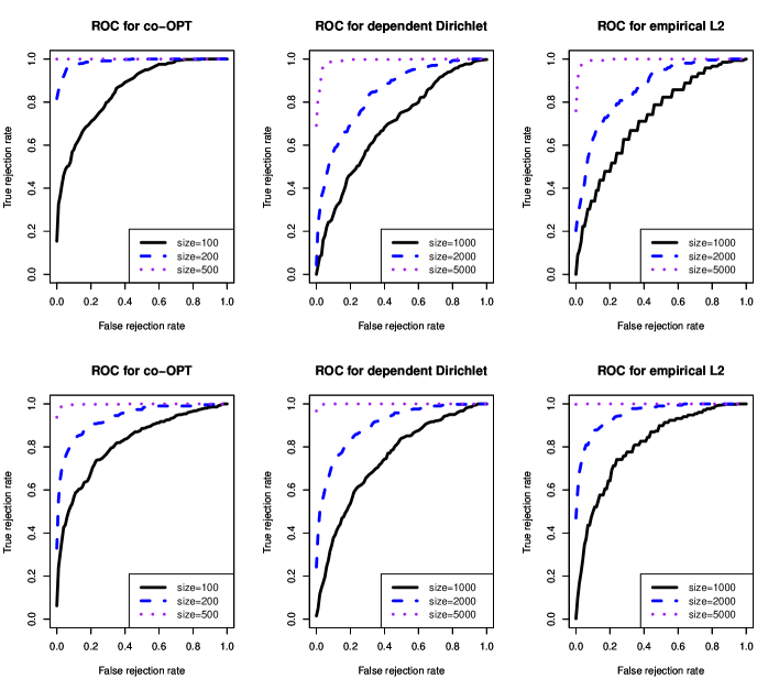
Example 5 (Retrospectively sampled data on a $2^{15}$ contingency table).

Suppose there are 15 binary predictors $X_{1},X_{2},\ldots,X_{15}$, and there is a binary response variable $Y$, e.g. disease status, whose distribution is

$$Y\sim\left\{\begin{array}[]{ll}Bernoulli(0.3)&\mbox{if $X_{3}=1$ and $X_{7}=1$}\\ Bernoulli(0.3)&\mbox{if $X_{7}=0$ and $X_{10}=0$}\\ Bernoulli(0.1)&\mbox{otherwise.}\end{array}\right.$$

We simulate populations for joint observations of $X_{i}$’s and $Y$ of size 200,000 under two scenarios

1. $X_{1},X_{2},\ldots,X_{15}$ $\sim_{i.i.d.}$ Bernoulli(0.5)

2. $X_{1},X_{2},\ldots X_{8}$ as a Markov Chain with $X_{1}\sim$ Bernoulli(0.5), and $P(X_{t}=X_{t-1}|X_{t-1})=0.7$, while $X_{9},X_{10},\ldots X_{15}$ $\sim_{i.i.d}$ Bernoulli(0.5) and are independent of $X_{1},\ldots,X_{8}$.

For each scenario, we retrospectively sample controls ($Y$=0) and cases ($Y$=1). Our interest is in (1) the power of our method in detecting the difference in the joint distribution of the predictor variables between the two samples, and (2) whether the method can recover the “interactive” structure among the three predictors $X_{3}$, $X_{7}$ and $X_{10}$.

We place two different priors on $(Q_{1},Q_{2})$ and compare their performance. The first is our co-OPT distribution with prior parameters being specified as in Example 1. The second is a dependent Dirithlet prior inspired by [14]. Under this setup we write $Q_{1}$ and $Q_{2}$ as mixtures, $Q_{1}=\epsilon H_{0}+(1-\epsilon)H_{1}$ and $Q_{2}=\epsilon H_{0}+(1-\epsilon)H_{2}$, where $H_{0}$ represents the common part of $Q_{1}$ and $Q_{2}$ while $H_{1}$ and $H_{2}$ the idiosyncratic portion. Under the prior, $H_{0}$, $H_{1}$ and $H_{2}$ $\sim_{i.i.d}Dirichlet({\bm{\alpha}_{H}})$ and $\epsilon\sim Beta(a_{\epsilon},b_{\epsilon})$. For the hyperparameters, we chose ${\bm{\alpha}_{H}}=(0.5,0.5,\ldots,0.5)$—that is, each cell in the support of the Dirichlet receives 0.5 prior pseuodocount, and $a_{\epsilon}=b_{\epsilon}=3$. We found that due to the sparsity of the table, restricting the prior to have a support over only the observed table cells rather than the entire table drastically improves the power. Therefore, this is what we do here. (More details about the prior specification and how MCMC sampling is used to draw posterior samples for this prior can be found in the supplementary materials.)

Because $\epsilon$ can be thought of as a measure of how similar $Q_{1}$ and $Q_{2}$ are, the mean of its posterior distribution can serve as a statistic (which we shall from now on refer to as the $\epsilon$-statistic) for testing the difference between the two. The ROC curves of the $\epsilon$-statistic, and that of our co-OPT statistic, for the two scenarios and different sample sizes are given in the left and middle columns of 3. For comparison, the right column of the figure gives the ROC curve for another statistic measuring two sample difference, namely the empirical $L_{2}$ distance between the two contingency tables corresponding to the cases and the controls. Note that in this example to achieve comparable performance the the $\epsilon$-statistic and the $L_{2}$ distance both require samples sizes 10 times as large as those for the co-OPT! This performance advantage of the co-OPT in this setting is probably due to (1) the adaptive partitioning feature and (2) the coupling feature, both of which help mitigate the difficulties caused by the sparsity of the table counts. Also interesting is the impact of the correlation among predictors on the power. For the co-OPT, the correlation structure in Scenario 2 makes it harder to find a good partition of the space and therefore reduces power. On the other hand, the performance of the $\epsilon$-statistic, as well as that of the $L_{2}$ distance, is actually better for Scenario 2, as the correlation structure turns a marginal association (marginal w.r.t. the subspace of $X_{3}$, $X_{7}$ and $X_{10}$) into a joint one involving $X_{1}$ through $X_{10}$.

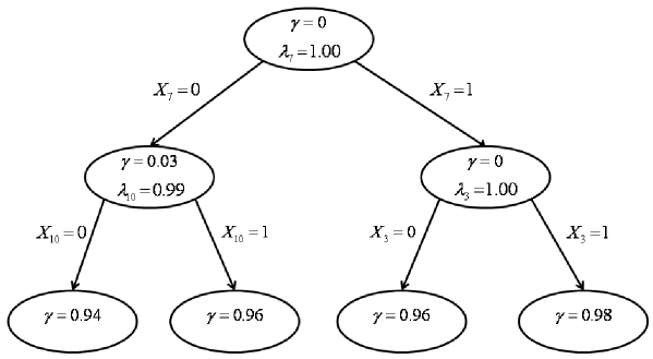
While the $\epsilon$-statistic and the $L_{2}$ distance can only serve for detecting the difference, the posterior co-OPT can also capture the underlying structure of the difference. We find that with about 500 data points in each sample for Scenario 1 and about 3500 data points in each sample for Scenario 2, the underlying structure can be accurately recovered using the hierarchical maximum a posteriori (hMAP) tree topology, which is a top-down stepwise posterior maximum likelihood tree. (The construction of the hMAP tree as well as the motivation to choose it over the MAP tree is discussed in detail in Section 4.2 of [17].) As one would expect, the correlation between the predictor variables makes it much harder to recover the exact interactive relation. A typical hMAP tree structure for the simulated populations with these sample sizes is given in 4. We note that in general a sample of partition trees from the posterior distribution of the tree structure can be more informative than the hMAP tree, especially when the sample sizes are not large enough. We use the hMAP here as a demonstration for its ease of visualization.

Figure 3: ROC curves of the co-OPT (left), the $\epsilon$ (middle), and the empirical $L_{2}$ (right) statistics for the two scenarios given in Example 4 (first row for Scenario 1 and second row for Scenario 2). The sample sizes for $\epsilon$ and $L_{2}$ are 10 times as large as those for the co-OPT.

Figure 4: A typical hMAP coupling tree that recovers the underlying interactive structure.

6   Inference on distributional distances between two samples

In some situations, one may be interested in a distance measure for the two sample distributions. For example, if we let $d(Q_{1},Q_{2})$ denote the distance between the two sample distributions under some metric $d$, one may want to compute quantities such as $P(d(Q_{1},Q_{2})>T|\bm{x}_{1},\bm{x}_{2})$ where $T$ is some constant. This can be achieved if one knows the posterior distribution of $d(Q_{1},Q_{2})$ or can sample from it. We next show that if $(Q_{1},Q_{2})$ arises from a co-OPT distribution, then for some common metrics, in particular $L_{1}$ and Hellinger distances, it is very convenient to sample from the distribution of $d(Q_{1},Q_{2})$.

As before, let $Q_{1}$ and $Q_{2}$ (with densities $q_{1}$ and $q_{2}$ respectively) be the two distributions of interest. Suppose $(Q_{1},Q_{2})$ have a co-OPT distribution, and so they can be thought of as being generated from the random-partitioning-and-assignment procedure introduced in the previous section through the drawing of the variables $C$, $J$, $\bm{\theta}_{1}$, $\bm{\theta}_{2}$, $C^{b}$, $J^{b}$ and $\bm{\theta}^{b}$. Then we have the following result.

Proposition 5.

Suppose $(Q_{1},Q_{2})$ has a co-OPT distribution satisfying the conditions given in Theorem 2. Let $\mathcal{A}(C,J)$ denote the (random) collection of all nodes on which $Q_{1}$ and $Q_{2}$ first couple. (The notation indicates that it depends on the coupling variables $C$ and $J$.) Also, let $d_{L_{1}}$ be the $L_{1}$ distance, and $d_{H^{2}}$ the squared Hellinger distance. (That is, $d_{L_{1}}(f,g)=\int|f-g|$ and $d_{H^{2}}(f,g)=\int(\sqrt{f}-\sqrt{g})^{2}$.) Then

$$d_{L_{1}}(Q_{1},Q_{2}) =\sum_{A\in\mathcal{A}(C,J)}|Q_{1}(A)-Q_{2}(A)|$$

$$d_{H^{2}}(Q_{1},Q_{2}) =\sum_{A\in\mathcal{A}(C,J)}(\sqrt{Q_{1}(A)}-\sqrt{Q_{2}(A)})^{2}.$$

Proof.

See supplementary materials. ∎

This proposition provides a recipe for drawing samples from the distributions of $d_{L_{1}}(Q_{1},Q_{2})$ and $d_{H^{2}}(Q_{1},Q_{2})$. One can first draw the coupling variables $C$, $J$, $\bm{\theta}^{1}$ and $\bm{\theta}^{2}$. Then use $C$ and $J$ to find the collection of nodes $\mathcal{A}(C,J)$, and use $\bm{\theta}^{1}$ and $\bm{\theta}^{2}$ to compute, for each $A\in\mathcal{A}(C,J)$, the corresponding measures $Q_{1}(A)$ and $Q_{2}(A)$. Finally, one draw of $d_{L_{1}}$ (or $d_{H^{2}}$) can be computed by summing $|Q_{1}(A)-Q_{2}(A)|$ (or $(\sqrt{Q_{1}(A)}-\sqrt{Q_{2}(A)})^{2}$) over all nodes in $\mathcal{A}(C,J)$.

A particularly desirable feature of this procedure for sampling $L_{1}$ and Hellinger distances is that one does not need to draw samples for the two random distributions $Q_{1}$ and $Q_{2}$ to get their distances. In fact, one only needs to draw the coupling variables, which characterize the difference between the two distributions, without having to draw the base variables, which characterize the fine structure of the two densities. Again, in multi-dimensional settings where estimating densities is difficult, such a procedure can produce much less variable samples for the distances.

We close this section with two more numerical examples, one in $\mathbb{R}$ and one in $\mathbb{R}^{2}$. In the second of these, again we use the observed range of the data in each dimension to define the space $\Omega$. Also, we use 1/10000 as the size cutoff for technical termination.

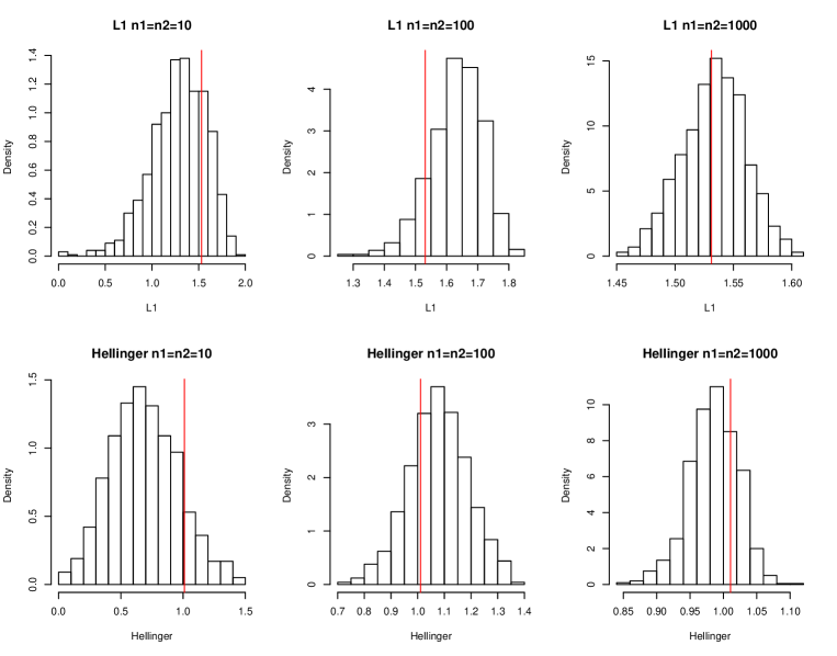
Example 6 (Two beta distributions).

We simulate two samples from Beta(2,5) and Beta(20,15) under three sets of sample sizes $n_{1}=n_{2}=$10, 100 and 1000. We place a co-OPT prior on the two distributions with the diadic partition rule and the symmetric parameter values as specified in Example 2 with $\rho_{0}=\gamma_{0}=0.5$, and compute the corresponding posterior co-OPT. Then we draw 1000 samples for each of $d_{L_{1}}(Q_{1},Q_{2})$ and $d_{H^{2}}(Q_{1},Q_{2})$ from their posterior distributions. The histograms of these samples are plotted in 5, where the vertical lines indicate the actual $L_{1}$ and squared Hellinger distances between the two distributions.

Figure 5: Histograms for posterior samples of $L_{1}$ and squared Hellinger distances for two samples from Beta(2,5) and Beta(20,15). The vertical lines indicate the actual $L_{1}$ and squared Hellinger distance between these two distributions.

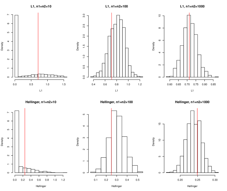
Example 7 (Bivariate normal and mixture of bivariate normal).

We repeat the same thing as in the previous example except now we simulate the two samples from the following distributions in $\mathbb{R}^{2}$.

Sample 1 $\sim BN\Biggl{(}\begin{pmatrix}0\\ 0\end{pmatrix},\begin{pmatrix}4&0\\ 0&4\\ \end{pmatrix}\Biggr{)}$, and

Sample 2 $\sim 0.5\times BN\Biggl{(}\begin{pmatrix}1\\ 1\end{pmatrix},\begin{pmatrix}1&0\\ 0&1\\ \end{pmatrix}\Biggr{)}+0.5\times BN\Biggl{(}\begin{pmatrix}-1\\ -1\end{pmatrix},\begin{pmatrix}1&0\\ 0&1\\ \end{pmatrix}\Biggr{)}$.

Again we draw 1000 posterior samples for $d_{L_{1}}(Q_{1},Q_{2})$ and for $d_{H^{2}}(Q_{1},Q_{2})$ under each set of sample sizes. The histograms of these samples are plotted in 6, where the vertical lines again indicate the actual $L_{1}$ and squared Hellinger distances between the two distributions.

Figure 6: Histograms for posterior samples of $L_{1}$ and squared Hellinger distances for Example 6. The vertical lines indicate the actual $L_{1}$ and squared Hellinger distances for the two underlying distributions.

7   Concluding remarks

In this work we have introduced the coupling optional Pólya tree prior for Bayesian nonparametric analysis on the two sample problem. This prior jointly generates two random probability distributions that can “couple” on subsets of the sample space. We have demonstrated that this construction allows both the testing and the learning of the distributional difference between the two samples. One can easily extend this prior to allow the joint generation of more than two samples. For example, if four samples are involved, then one can draw four, instead of two, independent Dirichlet vectors for probability assignment on each uncoupled node.

One interesting feature of the co-OPT prior (as well as the original OPT prior) is that the corresponding posterior can be computed “exactly” using the recursive formulation given in (4.5) without resorting to Markov Chain Monte Carlo sampling. However, such “exact inference” based on recursions is still computationally intensive, especially in high-dimensional problems. Efficient implementation is a necessity for this method to be feasible for any non-trivial problems. However, even with the most efficient implementation, the exponential nature of the method dictates that approximation techniques such as $k$-step look-ahead as well as large-scale parallelization are needed for very high dimensional problems, such as those on a contingency table with 100 dimensions. Current work is undergoing in this direction.

Acknowledgment

The authors want to thank Art Owen, David Siegmund, Hua Tang, Robert Tibshirani, four referees, and the editors for very helpful comments. LM is supported by a Larry Yung Stanford Interdisciplinary Graduate Fellowship. WHW is supported in part by NSF grant DMS-0906044. Much of the computation is done on systems supported by NSF SCREMS Grant DMS-0821823 and NSF award CNS-0619926.

Supplemental materials

Appendices

A.1 includes all the proofs. A.2 gives the details about the prior specifications for the comparison made in Example 4. A.3 gives the details about the specification of the dependent Dirichlet prior as well as the Gibbs sampler used for drawing posterior samples of $\epsilon$.

Appendix A.1. Proofs

Proof of Theorem 1.

Consider the RPAA procedure described in Section 2 with the uniform base distribution $u$ replaced by $q_{0}$. So under this new procedure of generating a random measure $Q$, whenever a region $A$ gets stopped, the conditional distribution of $Q$ within $A$ is set to be $Q_{0}(\cdot|A)$. Let $Q^{(k)}$ be the corresponding random distribution that is forced to stop after $k$ levels of nested partitioning. In other words, for all non-stopped nodes $A$ reached after $k$ levels of nested partitioning, we stop dividing $A$ regardless of the stopping variable $S(A)$ and force a conditional distribution $Q_{0}(\cdot|A)$ on it to obtain $Q^{(k)}$. (For more detail see the proof of Theorem 1 in [17].)

We first show that if $\alpha^{j}_{i}(A)/\sum_{h=1}^{K^{j}(A)}\alpha^{j}_{h}(A)=Q_{0}(A^{j}_{i})/Q_{0}(A)$, then $EQ^{(k)}(B)=Q_{0}(B)$ for all $k$. For $k\geq 0$, let $\mathcal{J}^{(k)}$ be the collection of all partition random variables $S$ and $J$ drawn in the first $k$ levels of partitioning, and let $\mathcal{A}(\mathcal{J}^{(k)})$ be the collection of all leaf nodes after $k$ levels of random partitioning—those are the nodes that are either just reached in the $k$th step or are reached earlier but stopped. We prove by induction that $E\left(Q^{(k)}(B)|\mathcal{J}^{(k)}\right)=Q_{0}(B)$. For $k=0$, $\mathcal{J}^{(k)}=\emptyset$, $\mathcal{A}(\mathcal{J}^{(k)})=\{\Omega\}$, and $Q^{(0)}=Q_{0}$ and so $E\left(Q^{(k)}(B)|\mathcal{J}^{(k)}\right)=Q_{0}(B)$ holds trivially. Now for $k\geq 1$, suppose this holds true for $1,2,\ldots,k-1$. By construction,

$$Q^{(k)}(B)=\sum_{A\in\mathcal{A}(\mathcal{J}^{(k)})}Q^{(k)}(A)\frac{Q_{0}(B\cap A)}{Q_{0}(A)}.$$

Let $A^{p}\in\mathcal{A}(\mathcal{J}^{(k-1)})$ be the parent node of $A$, that is, the node whose division gives rise to $A$. Then by the condition that $\alpha^{j}_{i}(A)/\sum_{h=1}^{K^{j}(A)}\alpha^{j}_{h}(A)=Q_{0}(A^{j}_{i})/Q_{0}(A)$, we have

$$E(Q^{(k)}(A)/Q^{(k)}(A^{p})|\mathcal{J}^{(k)})=Q_{0}(A)/Q_{0}(A^{p}),$$

and so

$$E\left(Q^{(k)}(B)|\mathcal{J}^{(k)}\right) =E\left(\sum_{A\in\mathcal{A}(\mathcal{J}^{(k)})}Q^{(k)}(A)\frac{Q_{0}(B\cap A)}{Q_{0}(A)}\Big{|}\mathcal{J}^{(k)}\right)$$

$$=\sum_{A\in\mathcal{A}(\mathcal{J}^{(k)})}\frac{Q_{0}(B\cap A)}{Q_{0}(A)}E\Biggl{(}Q^{(k)}(A)\Big{|}\mathcal{J}^{(k)}\Biggr{)}$$

$$=\sum_{A\in\mathcal{A}(\mathcal{J}^{(k)})}\frac{Q_{0}(B\cap A)}{Q_{0}(A)}E\Biggl{(}\frac{Q^{(k)}(A)}{Q^{(k)}(A^{p})}Q^{(k)}(A^{p})\Big{|}\mathcal{J}^{(k)}\Biggr{)}$$

$$=\sum_{A\in\mathcal{A}(\mathcal{J}^{(k)})}\frac{Q_{0}(B\cap A)}{Q_{0}(A)}\frac{Q_{0}(A)}{Q_{0}(A^{p})}E\Biggl{(}Q^{(k)}(A^{p})\Big{|}\mathcal{J}^{(k)}\Biggr{)}$$

$$=\sum_{A\in\mathcal{A}(\mathcal{J}^{(k)})}\frac{Q_{0}(B\cap A)}{Q_{0}(A^{p})}E\Biggl{(}Q^{(k-1)}(A^{p})\Big{|}\mathcal{J}^{(k)}\Biggr{)}$$

$$=\sum_{A\in\mathcal{A}(\mathcal{J}^{(k)})}Q_{0}(B\cap A)=Q_{0}(B).$$

This shows that $E\left(Q^{(k)}(B)|\mathcal{J}^{(k)}\right)=Q_{0}(B)$ and thus $EQ^{(k)}(B)=Q_{0}(B)$ for all $k$. But since $|Q^{(k)}(B)-Q(B)|\rightarrow 0$ a.s.​ (see the proof of Theorem 1 in [17]), by bounded convergence theorem, we have $E|Q^{(k)}(B)-Q(B)|\rightarrow 0$, and so $EQ(B)=Q_{0}(B)$. ∎

Proof of Theorem 2.

We first claim that with probability 1, $Q_{1}^{(k)}$ and $Q_{2}^{(k)}$ respectively converge in total variational distance to two absolutely continuous random probability measures $Q_{1}$ and $Q_{2}$, and thus for any Borel set $E$,

$$|Q_{1}^{(k)}(E)-Q_{1}(E)|+|Q_{2}^{(k)}(E)-Q_{2}(E)|$$

$$\leq \,sup_{E_{1}\in\mathcal{B}}|Q_{1}^{(k)}(E_{1})-Q_{1}(E_{1})|+sup_{E_{2}\in\mathcal{B}}|Q_{1}^{(k)}(E_{2})-Q_{1}(E_{2})|\rightarrow 0,\hbox{ w.p.1.}$$

To prove the claim, we note that the marginal procedure that generates $Q_{1}$, for instance, is simply an OPT with random local base measures that arise from standard OPT distributions. To see this, we can think of the generative procedure of $Q_{1}$ as consisting of the following two steps.

1. For each potential tree node $A$ under $\mathcal{R}$, we draw an independent random measure $Q_{0}^{A}$ from $OPT_{|A}(\mathcal{R},\rho,\bm{\lambda}^{b},\bm{\alpha}^{b})$.

2. Generate $Q_{1}$ from the standard random-partitioning-and-random-assignment procedure for an OPT, treating $\{C(A)\}$ as the stopping variables, $\{J(A)\}$ as the partition selector variables, and $\{\bm{\theta}^{J(A)}_{1}(A)\}$ as the probability assignment variables, and with $\{Q_{0}^{A}\}$ being the local base measures. That is, when a node $A$ is stopped, the conditional distribution $Q_{1}(\cdot|A)$ is set to be $Q_{0}^{A}(\cdot)$.

By Theorem 1 in [17], for each potential node $A$, with probability 1, $Q_{0}^{A}$ is an absolutely continuous distribution. Because the collection of all potential tree nodes $A$ under $\mathcal{R}$ is countable, with probability 1, this simultaneously holds for all $Q_{0}^{A}$. Therefore, with probability 1, the marginal procedure for producing $Q_{1}$ is just that for an OPT with local base measures $\{Q_{0}^{A}\}$. The same argument for proving Theorem 1 in [17] (with $\mu(\cdot|A)$ replaced by $Q_{0}^{A}(\cdot)$) shows that with probability 1, an absolutely continuous measure $Q_{1}$ exists as the limit of $Q_{1}^{(k)}$ in total variational distance. The same argument proves the claim for $Q_{2}$ as well. ∎

Proof of Theorem 3.

Because any density function on $\Omega$ can be arbitrarily approximated in $L_{1}$ by uniformly continuous ones, without loss of generality, we can assume that $f_{1}$ and $f_{2}$ are uniformly continuous. Let

$$\delta_{1}(\epsilon)=\sup_{|x-y|<\epsilon}|f_{1}(x)-f_{1}(y)|\quad\text{and}\quad\delta_{2}(\epsilon)=\sup_{|x-y|<\epsilon}|f_{2}(x)-f_{2}(y)|.$$

By uniform continuity, we have $\delta_{i}(\epsilon)\downarrow 0$ as $\epsilon\downarrow 0$ for $i=1,2$. Also, by Condition (1), for any $\epsilon>0$, there exists a partition of $\Omega=\cup_{i=1}^{I}A_{i}$ such that the diameter of each $A_{i}$ is less than $\epsilon$. By Condition (2), there is positive probability that this partition will arise after a finite number of steps of recursive partitioning. Also because the parameters of the co-OPT are all bounded away from 0 and 1, there is a positive probability that the $A_{i}$’s are exactly the sets on which $Q_{1}$ and $Q_{2}$ first couple. Now let $q^{A_{i}}$ be the local base measure on each of $A_{i}$, we can write

$$q_{1}(x)=\sum_{i=1}^{I}Q_{1}(A_{i})q^{A_{i}}(x){\mathbf{1}}_{A_{i}}(x)\quad\text{and}\quad q_{2}(x)=\sum_{i=1}^{I}Q_{2}(A_{i})q^{A_{i}}(x){\mathbf{1}}_{A_{i}}(x).$$

Accordingly,

$$\,\,\,\,\,\int|q_{1}(x)-f_{1}(x)|d\mu(x)$$

$$=\sum_{i=1}^{I}\int_{A_{i}}|Q_{1}(A_{i})q^{A_{i}}(x)-f_{1}(x)|d\mu(x)$$

$$\leq\sum_{i=1}^{I}Q_{1}(A_{i})\int_{A_{i}}|q^{A_{i}}(x)-1/\mu(A_{i})|d\mu(x)+\sum_{i=1}^{I}\int_{A_{i}}|Q_{1}(A_{i})/\mu(A_{i})-f_{1}(x)|d\mu(x)$$

$$\leq\sum_{i=1}^{I}\int_{A_{i}}|q^{A_{i}}(x)\!-\!1/\mu(A_{i})|d\mu(x)\!+\!\sum_{i=1}^{I}|Q_{1}(A_{i})\!-\!f_{1}^{i}\,\mu(A_{i})|\!+\!\sum_{i=1}^{I}\int_{A_{i}}|f_{1}^{i}\!-\!f_{1}(x)|d\mu(x)$$

where $f_{1}^{j}:=\int_{A_{i}}f_{1}(x)d\mu(x)/\mu(A_{i})$. By the exact same calculation we have

$$\,\,\,\,\,\int|q_{2}(x)-f_{2}(x)|d\mu(x)$$

$$\leq\sum_{i=1}^{I}\int_{A_{i}}|q^{A_{i}}(x)\!-\!1/\mu(A_{i})|d\mu(x)\!+\!\sum_{i=1}^{I}|Q_{2}(A_{i})\!-\!f_{2}^{i}\,\mu(A_{i})|+\sum_{i=1}^{I}\int_{A_{i}}|f_{2}^{i}\!-\!f_{2}(x)|d\mu(x)$$

where $f_{2}^{j}:=\int_{A_{i}}f_{2}(x)d\mu(x)/\mu(A_{i})$. By the choice of $A_{i}$, we have that $\int_{A_{i}}|f_{1}^{i}-f_{1}(x)|d\mu(x)\leq\delta_{1}(\epsilon)\mu(A_{i})$ and $\int_{A_{i}}|f_{2}^{i}-f_{2}(x)|d\mu(x)\leq\delta_{2}(\epsilon)\mu(A_{i})$. Thus,

$$\sum_{i=1}^{I}\int_{A_{i}}|f_{1}^{i}-f_{1}(x)|d\mu(x)\leq\delta_{1}(\epsilon)\mu(\Omega)\quad\text{and}\quad\sum_{i=1}^{I}\int_{A_{i}}|f_{2}^{i}-f_{2}(x)|d\mu(x)\leq\delta_{2}(\epsilon)\mu(\Omega).$$

So by choosing $\epsilon$ small enough, we can have

$$\max\{\delta_{1}(\epsilon),\delta_{2}(\epsilon)\}\mu(\Omega)<\tau/3.$$

Next, because all the coupling parameters of the co-OPT prior are uniformly bounded away from 0 and 1, (conditional on the coupling partition) with positive probability, we have

$$|Q_{1}(A_{i})-f_{1}^{i}\,\mu(A_{i})|<\frac{\tau}{3\mu(\Omega)}\quad\text{and}\quad|Q_{2}(A_{i})-f_{2}^{i}\,\mu(A_{i})|<\frac{\tau}{3\mu(\Omega)}$$

for all $i=1,2,\ldots,I$. Similarly, because all the base parameters are also uniformly bounded away from 0 and 1, by Theorem 2 in [17], (conditional on the coupling partition and probability assignments,) with positive probability we have

$$\int_{A_{i}}|q^{A_{i}}(x)-1/\mu(A_{i})|d\mu(x)<\frac{\tau}{3\cdot 2^{i}}$$

for all $i=1,2,\ldots,I$. Placing the three pieces together, we have positive probability for $\int|q_{1}(x)-f_{1}(x)|d\mu<\tau$ and $\int|q_{2}(x)-f_{2}(x)|d\mu<\tau$ to hold simultaneously. ∎

Proof of Proposition 5.

We prove the result only for $d_{L_{1}}$ as the proof for $d_{H^{2}}$ is very similar. (All following equalities and statements hold with probability 1.)

$$d_{L_{1}}(Q_{1},Q_{2}) =\int_{\Omega}|q_{1}(x)-q_{2}(x)|\mu(dx)$$

$$=\sum_{A\in\mathcal{A}(C,J)}\int_{A}|q_{1}(x)-q_{2}(x)|\mu(dx)+\int_{\Omega\setminus\,\cup\mathcal{A}(C,J)}|q_{1}(x)-q_{2}(x)|\mu(dx).$$

But for each $A\in\mathcal{A}(C,J)$, due to coupling we have $q_{1}(\cdot|A)=q_{2}(\cdot|A)$, and so

$$\int_{A}|q_{1}(x)-q_{2}(x)|\mu(dx) =\int_{A}|Q_{1}(A)-Q_{2}(A)|q_{1}(x|A)\mu(dx)$$

$$=|Q_{1}(A)-Q_{2}(A)|.$$

On the other hand, $Q_{1}(\Omega\setminus\cup\mathcal{A}(C,J))=Q_{2}(\Omega\setminus\cup\mathcal{A}(C,J))=\mu(\Omega\setminus\cup\mathcal{A}(C,J))=0$ w.p.1. (See proof of Theorem 1 in [17].) Therefore,

$$d_{L_{1}}=\sum_{A\in\mathcal{A}(C,J)}|Q_{1}(A)-Q_{2}(A)|.$$

∎

Appendix A.2. Prior specifications for Example 4

For the Pólya tree two sample test [10], we have imposed that each tree node is partitioned in the middle of both dimensions at each level. Therefore for our example in $\mathbb{R}^{2}$, each node has four children. We also impose that the prior pseudo-counts $\alpha$ are 0.5 for all children. The software used in this paper for this method is written by us.

On the other hand, we used R package DPpackage function HDPMdensity to fit the Dirichlet Process mixture (DPM) model proposed in [14]. More specifically, the two distributions are modeled as.

$$F_{1} =\epsilon H_{0}+(1-\epsilon)H_{1}$$

$$F_{2} =\epsilon H_{0}+(1-\epsilon)H_{2},$$

where $H_{0}$ models the common part of $F_{1}$ and $F_{2}$, whereas $H_{1}$ and $H_{2}$ the unique parts. The parameter $\epsilon$ captures the proportion of“commonnes” between the two distributions, and thus can serve as a measure of how the two differ. Each of the $H_{i}$ for $i=0,1,2$ is modeled as a Dirichlet Process mixture of normals.

$$H_{i}(\cdot)=\int\phi(\cdot|\mu,\Sigma)dG_{i}(\mu),$$

where

$$G_{i}|\alpha_{i},G_{0}\sim DP(\alpha_{i},G_{0}).$$

The baseline distribution $G_{0}$ is assumed to be $Normal(\mu_{0},\Sigma_{0})$. Following the example given by DPpackage, the (empirical) hyperprior specifications are

$$\epsilon \sim 0.1\delta_{0}+0.1\delta_{1}+0.8\,Unif[0,1],$$

$$\alpha_{i} \sim Unif(0,1)\text{ for $i=0,1,2$.}$$

$$\Sigma_{0}|\mu_{0},T_{0} \sim InverseWishart(\mu_{0}=9,T_{0}={\rm Var}(\bm{y}))$$

$$\mu_{0}|m_{0},S_{0} \sim N(m_{0}=mean(\bm{y}),S_{0}={\rm Var}(\bm{y}))$$

$$\Sigma|\nu,T \sim InverseWishart(\nu=9,T=0.25{\rm Var}(\bm{y})),$$

where $\bm{y}$ is the combination of the two samples, $mean(\cdot)$ is the dimension-wise average, and ${\rm Var}$ is the covariance. The statistic we use to measure two sample difference (or similarity) is the posterior mean of $\epsilon$, estimated by the mean of the MCMC sample of size 10,000, with 10,000 burn-in steps.

Appendix A.3. The dependent Dirichlet prior in Example 5

Motivated by the hierarchical Dirichlet process mixture prior setup introduced in [14], we can design the following prior for $(Q_{1},Q_{2})$ on the finite support of a contingency table.

$$\left\{\begin{array}[]{l}Q_{1}=\epsilon H_{0}+(1-\epsilon)H_{1}\\ Q_{2}=\epsilon H_{0}+(1-\epsilon)H_{2}\end{array}\right.$$

with

$$H_{0},H_{1},H_{2} \sim_{i.i.d}Dirichlet({\bm{\alpha}_{H}})$$

$$\epsilon \sim Beta(a_{\epsilon},b_{\epsilon}).$$

We used ${\bm{\alpha}_{H}}=(0.5,0.5,\ldots,0.5)$ and $a_{\epsilon}=b_{\epsilon}=3$ as the prior parameters. We found that restricting the support of $\alpha_{H}$ to the observed table cells rather than the entire table significantly improves the power of the method. This is due to the sparsity of the table counts—the vast majority of the table cells are empty.

To draw posterior samples of $\epsilon$, we use the following Gibbs sampler. First some notations. Let ${\bm{X}^{1}}=\{X^{1}_{1},X^{1}_{2},\ldots,X^{1}_{n_{1}}\}$ and ${\bm{X}^{2}}=\{X^{2}_{1},X^{2}_{2},\ldots,X^{2}_{n_{2}}\}$ denote the two sample observations. For each observation $X^{i}_{j}$ in sample $i=1$ or 2, we introduce a Bernoulli variable $J^{i}_{j}$ that serves as an indicator for whether $X_{i}^{j}$ has come for $H_{i}$ or $H_{0}$. Given $\epsilon$, the $J^{i}_{j}$’s are i.i.d. $Bernoulli(\epsilon)$ variables. For simplicity, we denote $(J^{i}_{1},J^{i}_{2},\ldots,J^{i}_{n_{i}})$ as ${\bm{J}^{i}}$. Given $\bm{J}^{i}$ we let

$$\bm{X}^{i,0}=\{X^{i}_{j}:J^{i}_{j}=0,j=1,2,\ldots,n_{i}\}\quad\text{ and }\quad\bm{X}^{i,1}=\{X^{i}_{j}:J^{i}_{j}=1,j=1,2,\ldots,n_{i}\}$$

for $i=1,2$. In addition, we let $\bm{n}(\bm{X}^{i})$ be the table counts of of sample $i$ in the support of $\bm{\alpha}_{H}$, and similarly define $\bm{n}(\bm{X}^{i,0})$ and $\bm{n}(\bm{X}^{i,1})$. With these notations, now we next write down the conditional distributions of $H_{0}$, $H_{1}$, $H_{2}$, $\epsilon$, $\bm{J}^{1}$ and $\bm{J}^{2}$.

$$H_{0}|\bm{X}^{1},\bm{X}^{2},\bm{J}^{1},\bm{J}^{2},\epsilon,H_{1},H_{2} \sim Dirichlet(\bm{\alpha}_{H}+\bm{n}(\bm{X}^{1,0})+\bm{n}(\bm{X}^{2,0}))$$

$$H_{1}|\bm{X}^{1},\bm{X}^{2},\bm{J}^{1},\bm{J}^{2},\epsilon,H_{0},H_{2} \sim Dirichlet(\bm{\alpha}_{H}+\bm{n}(\bm{X}^{1,1}))$$

$$H_{2}|\bm{X}^{1},\bm{X}^{2},\bm{J}^{1},\bm{J}^{2},\epsilon,H_{0},H_{1} \sim Dirichlet(\bm{\alpha}_{H}+\bm{n}(\bm{X}^{2,1}))$$

$$J^{1}_{j}|\bm{X}^{1},\bm{X}^{2},\bm{J}^{1}_{(-j)},\bm{J}^{2},\epsilon,H_{0},H_{1},H_{2} \sim Bernoulli\left(\frac{(1-\epsilon)p_{H_{1}}(X^{1}_{j})}{\epsilon p_{H_{0}}(X^{1}_{j})+(1-\epsilon)p_{H_{1}}(X^{1}_{j})}\right)$$

$$J^{2}_{j}|\bm{X}^{1},\bm{X}^{2},\bm{J}^{1},\bm{J}^{2}_{(-j)},\epsilon,H_{0},H_{1},H_{2} \sim Bernoulli\left(\frac{(1-\epsilon)p_{H_{1}}(X^{1}_{j})}{\epsilon p_{H_{0}}(X^{1}_{j})+(1-\epsilon)p_{H_{1}}(X^{1}_{j})}\right)$$

$$\epsilon|\bm{X}^{1},\bm{X}^{2},\bm{J}^{1},\bm{J}^{2},H_{0},H_{1},H_{2} \sim Beta\left(a_{\epsilon}+\sum_{i=1}^{2}\sum_{j=1}^{n_{i}}J^{i}_{j},\,\,b_{\epsilon}+n_{1}+n_{2}-\sum_{i=1}^{2}\sum_{j=1}^{n_{i}}J^{i}_{j}\right).$$

We use this Gibbs sampler to draw posterior samples for $\epsilon$. We compute the posterior mean of $\epsilon$ from $10,000$ samples with $10,000$ burn-in iterations.

References

- [1] Anderson, T. W. (1962). On the distribution of the two-sample Cramer-von Mises criterion. Ann. Math. Stat. 33, 3, 1148–1159.
- [2] Baringhaus, L. and Franz, C. (2004). On a new multivariate two-sample test. J. Multivar. Anal. 88, 1, 190–206.
- [3] Basu, S. and Chib, S. (2003). Marginal likelihood and bayes factors for dirichlet process mixture models. Journal of the American Statistical Association 98, 461, 224–235.
- [4] Berger, J. O. and Guglielmi, A. (2001). Bayesian and conditional frequentist testing of a parametric model versus nonparametric alternatives. Journal of the American Statistical Association 96, 453, 174–184.
- [5] Carota, C. and Parmigiani, G. (1996). On Bayes factors for nonparametric alternatives. In Bayesian statistics 5, J. M. Bernardo, J. O. Berger, A. P. Dawid, and A. F. M. Smith, Eds. Oxford University Press, 507–511.
- [6] Chakravarti, I. M., Laha, R. G., and Roy, J. (1967). Handbook of Methods of Applied Statistics. Vol. I. John Wiley and Sons, USE.
- [7] Florens, J. P., Richard, J. F., and Rolin, J. M. (1996). Bayesian encompassing specification tests of a parametric model against a non parametric alternative. Technical Report 96.08, Université Catholique de Louvain, Institut de statistique.
- [8] Griffin, J. and Steel, M. (2006). Order-based dependent dirichlet processes. Journal of the American Statistical Association 101, 179–194.
- [9] Hanson, T. E. (2006). Inference for mixtures of finite pólya tree models. Journal of the American Statistical Association 101, 1548–1565.
- [10] Holmes, C. C., Caron, F., Griffin, J. E., and Stephens, D. A. (2009). Two-sample Bayesian nonparametric hypothesis testing. http://arxiv.org/abs/0910.5060.
- [11] Lehmann, E. L. and Romano, J. P. (2006). Testing Statistical Hypotheses. Springer, New York.
- [12] MacEachern, S. (1999). Dependent dirichlet processes. In Proceedings of the section on Bayesian Statistical Science.
- [13] McVINISH, R., Rousseau, J., and Mengersen, K. (2009). Bayesian goodness of fit testing with mixtures of triangular distributions. Scandinavian Journal of Statistics 36, 2, 337–354.
- [14] Müller, P., Quintana, F., and Rosner, G. (2004). A method for combining inference across related nonparametric bayesian models. Journal of The Royal Statistical Society Series B 66, 3, 735–749.
- [15] Teh, Y. W., Jordan, M. I., Beal, M. J., and Blei, D. M. (2006). Hierarchical dirichlet processes. Journal of the American Statistical Association 101, 1566–1581.
- [16] Tokdar, S. T., Chakrabarti, A., and Ghosh, J. K. (2010). Bayesian non-parametric goodness of fit tests. In Frontiers of Statistical Decision Making and Bayesian Analysis, M.-H. Chen, D. K. Dey, P. Mueller, D. Sun, and K. Ye, Eds.
- [17] Wong, W. H. and Ma, L. (2010). Optional Pólya tree and Bayesian inference. Annals of Statistics 38, 3, 1433–1459. http://projecteuclid.org/euclid.aos/1268056622.