Interface-Mediated Interactions: Entropic Forces of Curved Membranes

Abstract

Particles embedded in a fluctuating interface experience forces and torques mediated by the deformations and by the thermal fluctuations of the medium. Considering a system of two cylinders bound to a fluid membrane we show that the entropic contribution enhances the curvature-mediated repulsion between the two cylinders. This is contrary to the usual attractive Casimir force in the absence of curvature-mediated interactions. For a large distance between the cylinders, we retrieve the renormalization of the surface tension of a flat membrane due to thermal fluctuations.

I Introduction

Particles bound to an interface may interact via forces and torques of two distinct physical origins. One contribution to these so-called interface-mediated interactions is purely geometric and results from the deformations caused by the particles. Since the interface is also a thermally fluctuating medium, embedded particles may also interact through a fluctuation-induced interaction. The associated entropic force is an example of the more general phenomenon of Casimir forces between objects placed in a fluctuating medium. In its original formulation, two uncharged conducting plates were predicted to attract each other due to the quantum electromagnetic fluctuations of the vacuum CASIMIR . In a soft matter context, fluctuation-mediated forces were, for instance, studied for objects immersed in a fluid near its critical point FisherdeGennes ; Hertleinetal ; Kresch or attached to a fluid interface LiKardar ; Dietrich ; NoruzifarOettel .

Interface-mediated forces have also received intense attention recently due to their possible relevance in biological processes: membrane-mediated interactions could aid cooperation of proteins in the biological membrane and complement the effects of direct van der Waals’ or electrostatic forces MARTINNATURE . Theoretical studies of this problem have typically considered particles on quasi-planar fluid membranes GOULIAN ; GOLESTANIAN ; PARKLUBENSKY ; KIMNEUOSTER ; FOURNIER ; WEIKL ; MarkusCasimir ; RoyaCasimir neglecting the intrinsic nonlinearity of the underlying (ground state) shape equation. Some systems, especially those with a symmetry, have been studied on a nonlinear level without taking into account any fluctuations BisBis .

In this paper, we investigate interface-mediated interactions in their full generality on a curved geometry including entropic contributions for the specific problem of two parallel cylinders bound to the same side of a membrane. The ground state of this problem and thus the forces at zero temperature induced by the membrane were studied in Refs. MARTIN2005 ; MARTIN2007 via stress and torque tensors and in Refs. MARTIN2007 ; MkrtchyanIngChen via energy minimization. The method employed here to include thermal fluctuations is based on the calculation of the free energy of the system in a semi-classical approximation, where Gaussian fluctuations around the curved ground state are computed. To this end we introduce a new parametrization for the fluctuation variables which is possible due to the translational symmetry of the membrane. The force can then be obtained by deriving the free energy with respect to the distance between the cylinders.

II The model

We first start by exposing the problem and shortly retrieve the ground state configuration which will be the starting point for the computation of the thermal fluctuations. Consider two identical cylinders of length $L$ and radius $R$ bound to one side of the membrane, parallel to the $y$ axis and separated by a distance $d$ (see Fig. 1).

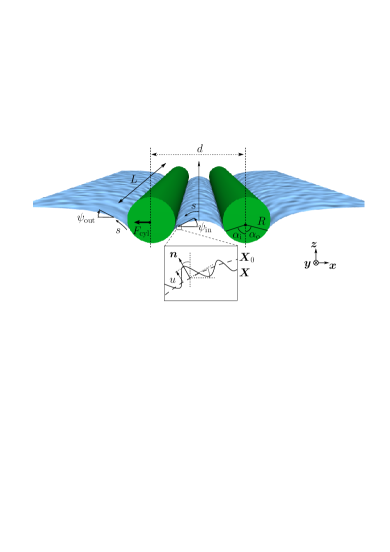
Figure 1: (Color online) Two parallel cylinders on the same side of a fluid membrane with fixed wrapping angle $\alpha_{\text{c}}=\alpha_{\text{i}}+\alpha_{\text{o}}=120^{\circ}$. The membrane fluctuates around its ground state profile ${\bm{X}}_{0}$. The corresponding fluctuation variable $u$ gives the distance between ${\bm{X}}_{0}$ and the actual profile ${\bm{X}}$ measured along the normal ${\bm{n}}$ of the ground state membrane (see inset).

In the limit of large $L/R$, boundary effects at the ends of the cylinders can be neglected and the profile can be decomposed into the following parts: an inner section between the cylinders, two outer sections that become flat for $x\rightarrow\pm\infty$, and two bound sections in which the cylinder and the membrane are in contact with each other. The contact area is given by $\alpha_{\text{c}}RL$ where $\alpha_{\text{c}}$ is the wrapping angle (see Fig. 1). The value of $\alpha_{\text{c}}$ depends on the physical situation considered: $i)$ the cylinder either has a finite adhesion energy $w$ per area so that $\alpha_{\text{c}}$ is determined via an adhesion balance at the contact lines or $ii)$ only a given part of the cylinder surface is adhering strongly to the membrane so that $\alpha_{\text{c}}$ is fixed. The ground state of case $i)$, which was studied numerically in detail in Ref. MkrtchyanIngChen , displays a phase diagram which is more complicated than in case $ii)$. In order to avoid complications already at the ground state level we will thus focus on case $ii)$ in the following by setting $\alpha_{\text{c}}=\alpha_{\text{o}}+\alpha_{\text{i}}=\text{const}$, where $\alpha_{\text{o}/\text{i}}$ is the contact angle between the cylinder and the outer/inner membrane. The shape of the bound parts is prescribed by the geometry of the attached cylinder, whereas the profiles of the free membrane sections are determined by solving the nonlinear shape equation which results from the minimization of the Helfrich Hamiltonian Canham ; Helfrich

$$H=\int_{\Sigma}\text{d}A\,\left(\sigma+\frac{\kappa}{2}K^{2}\right)\;,$$ (1)

where $\Sigma$ is the surface of the free membrane and $\text{d}A$ is the infinitesimal area element. In this functional, $\sigma$ denotes the surface tension, $\kappa$ the bending rigidity, and $K$ the local curvature of the membrane. At zero temperature the profile obeys translational symmetry along the $y$ axis. It is thus convenient to introduce the angle-arc length parametrization $\psi(s)$ where $s$ is the arc length and $\psi$ the angle between the $x$ axis and the tangent to the profile. In this parametrization the curvature is given by $K=\pm\text{d}\psi/\text{d}s$ [$+$ for the inner region and $-$ for the outer ones (see again Fig. 1)]. The shape equation of the surface can be written as $\lambda^{2}\text{d}^{2}\psi/\text{d}s^{2}-\eta\sin\psi=0$ with $\lambda=\sqrt{\kappa/\sigma}$ the reference length scale. The dimensionless quantity $\eta$ is defined as $\eta=f_{x}/\sigma$, where $f_{x}$ is the force per length $L$ of the cylinder at every point of the membrane (which is constant and horizontal on each membrane section). Using the stress tensor MARTIN2007 , the zero temperature force on the left cylinder is given by the simple expression $F_{\text{cyl}}^{(0)}=\sigma(\eta-1)L$. The outer section exercises a pulling force $-\sigma L$ on the left cylinder, the force of the inner section is $\sigma\eta L$. Later on, we will see how the values of the forces will be renormalized by thermal fluctuations. For the total force without fluctuations one only has to determine the value of $\eta$ which is an implicit function of $d.$ To do so, one first solves the shape equation which admits different solutions $\psi_{\text{in}}(s)$ and $\psi_{\text{out}}(s)$ (expressed in terms of elliptic Jacobi functions) corresponding to the inner and outer sections and depending on the boundary conditions at each cylinder. The value of $\eta$ in the inner section for any given $\alpha_{\text{i}}$ is determined implicitly by the requirement $\psi_{0}\equiv\psi_{\text{in}}(s_{0})=\alpha_{\text{i}}$ where $s_{0}$ is the arc length between the mid-line and the contact point on the cylinder of the inner membrane. Then $s_{0}$ is also implicitly determined by the relation

$$\frac{d}{2}-R\sin\alpha_{\text{i}}=\int_{0}^{s_{0}}\text{d}s\cos\psi\;.$$ (2)

The torque balance equation at equilibrium,

$$K_{\text{i}}-K_{\text{o}}-\frac{R}{\lambda^{2}}(\eta\cos{\alpha_{\text{i}}}-\cos{\alpha_{\text{o}}})=0\;,$$ (3)

where $K_{\text{o}/\text{i}}$ is the contact curvature in the outer/inner region, fixes the individual values $\alpha_{\text{o}}$ and $\alpha_{\text{i}}$. Solving the torque equation, values of $\eta$, $\alpha_{\text{o}}$, $\alpha_{\text{i}}$ for a given $d$ can now be determined numerically. For the case under consideration $\eta<1$ is an increasing function with the distance $d$ so that the cylinders always repel each other MARTIN2007 . This justifies that we have restricted our discussion to parallel cylinders. Indeed, every deviation from parallelism would directly be compensated by a counteracting torque.

III Thermal fluctuations

III.1 The fluctuation operator $H^{(2)}$

With the knowledge of the zero temperature profile, it is now possible to compute the entropic force. We first focus on the inner section and set $\psi(s)\equiv\psi_{\text{in}}(s)$. The position vector including fluctuations can then be written as ${\bm{X}}(s,y)={\bm{X}}_{0}(s)+(-u\sin{\psi},0,u\cos{\psi})$ where $u(s,y)$ is the membrane fluctuation in the normal direction and ${\bm{X}}_{0}(s)$ the position vector of the zero temperature profile (see inset of Fig. 1).

For small temperature the Helfrich Hamiltonian (1) can be expanded $H=H_{0}+H^{(2)}$ to second order in $u$, where $H_{0}$ is the ground state energy. The contribution $V(d)$ of the fluctuations to the free energy is then given by:

$$V(d)=\beta^{-1}\ln\int\text{D}u\,e^{-\beta H^{(2)}}\;,$$ (4)

where $\beta^{-1}=k_{B}T$. The fluctuation operator $H^{(2)}$ can be determined by expressing the Helfrich Hamiltonian (1) with the help of the parametrization ${\bm{X}}(s,y)$. One obtains (see appendix A)

$$H^{(2)} = \int\left[\frac{\dot{\psi}^{4}u^{2}}{2}+\dot{\psi}\ddot{\psi}u_{s}u+\Big{(}\frac{1}{\lambda^{2}}+\frac{3\dot{\psi}^{2}}{2}\Big{)}\frac{u_{s}^{2}}{2}+\dot{\psi}^{2}u_{ss}u\right.$$ (5)

$$\left.+\frac{u_{ss}^{2}+u_{yy}^{2}}{2}+u_{ss}u_{yy}+\Big{(}\frac{1}{\lambda^{2}}-\frac{\dot{\psi}^{2}}{2}\Big{)}\frac{u_{y}^{2}}{2}\right]\text{d}s\text{d}y\;,$$

where $u$ was assumed to satisfy periodic boundary conditions. The domain of integration is $-L/2<y<L/2$ and $-s_{0}<s<s_{0}.$ The thermal contribution to the force of the inner section is in principal given by $F_{\text{in}}^{\text{fl}}=\partial V(d)/\partial d$. However, thermal fluctuations also induce a rotation of the cylinders to maintain the torque balance. For small membrane curvatures the actual values of $\eta$ as well as $s_{0}$ and $\psi_{0}$ differ only slightly from their zero temperature values. Solving the arc length and torque equations (2) and (3) for small deviations $\delta\eta$, $\delta s_{0}$, $\delta\psi_{0}$, one can see that the inner thermal force must be corrected by a prefactor, $i.e.$, $Z(\psi_{0},\eta)F_{\text{in}}^{\text{fl}}$. It turns out that $Z(\psi_{0},\eta)$ does not vary much from unity and is thus disregarded here. For a large curvature of the inner membrane this approximation would in principle break down even though a general change of the behavior is not expected.

The computation of Eq. (4) for every value of separation $d$ is very difficult as $H^{(2)}$ has no known eigenvalues and eigenfunctions. To circumvent this problem we focus on the two limiting cases, the quasi-flat and the highly curved regime and propose an interpolating formula for intermediate separations.

III.2 The quasi-flat regime

Let us first consider the quasi-flat regime, i.e., the regime of very large $d/\lambda$ for which the membrane can be considered as flat except at the cylinders. In this case $\eta\approx 1$ and $\partial\psi_{0}/\partial d\approx 0$. In Eq. (4) $u$ can be expanded in Fourier modes $u(s,y)=\sum_{q,n}u_{n,q}\exp(i\pi ns/s_{0})\exp(i\pi qy/L)$ with $n$ and $q$ two integers. An implicit cut-off $\Lambda$ of the order of the inverse of the membrane thickness ($a\sim 5\text{nm}$) is assumed. The number of modes along the $y$ -/$s$-direction are given respectively by $N=2\pi\Lambda L$ and $M=4\pi\Lambda s_{0}$ ($2s_{0}\approx d$ being the arc length of the inner part). Since the field $u(s,y)$ is dimensional, the measure of the partition function is $\text{D}u\equiv\prod_{y,s}\mu^{-1}\text{d}u(s,y)$ with $\mu$ an arbitrary length scale which disappears from the expression of the force.

To compute the energy contribution (4) in the quasi-flat regime, we decompose Eq. (5) in two parts:

$$H^{(2)} = \int\left[\frac{u_{ss}^{2}+u_{yy}^{2}}{2}+u_{ss}u_{yy}+\frac{1}{\lambda^{2}}\frac{u_{y}^{2}}{2}\right]\text{d}s\text{d}y$$ (6)

$$\,+\,\int\left[\frac{\dot{\psi}^{4}u^{2}}{2}+\dot{\psi}\ddot{\psi}u_{s}u+\Big{(}\frac{1}{\lambda^{2}}+\frac{3\dot{\psi}^{2}}{2}\Big{)}\frac{u_{s}^{2}}{2}+\dot{\psi}^{2}u_{ss}u-\frac{\dot{\psi}^{2}}{2}\frac{u_{y}^{2}}{2}\right]\text{d}s\text{d}y\;$$

and rewrite $H^{(2)}$ in Fourier components according to this decomposition:

$$H^{(2)}=4dL\beta\mu^{2}\sum_{m,n}u\left(-m\right)\left[\text{{G${}^{-1}$}}(-m,n,q)+{\text{{X}}}(-m,n,q)\right]u\left(n\right)\;,$$ (7)

where the $u(n)$ are the Fourier components of $u$, with $u(-m)=\bar{u}(m)$. The terms G^-1 and X correspond to the Fourier transform of the two terms arising in the decomposition (6). Namely, one has:

$$\text{{G${}^{-1}$}}(-m,n,q)=\delta_{mn}\left\{\left[\Big{(}\frac{\pi n}{d}\Big{)}^{2}+\Big{(}\frac{\pi q}{L}\Big{)}^{2}\right]^{2}+\frac{1}{\lambda^{2}}\left[\Big{(}\frac{\pi n}{d}\Big{)}^{2}+\Big{(}\frac{\pi q}{L}\Big{)}^{2}\right]\right\}\;,$$ (8)

which is the diagonal propagator of the flat case and

$${\text{{X}}}(-m,n,q) =\frac{1}{d}\int_{-\frac{d}{2}}^{\frac{d}{2}}{\text{d}}s\;\Bigg{[}\frac{1}{2}\dot{\psi}^{4}+\frac{3}{2}\left(\ddot{\psi}^{2}+\frac{1}{\lambda^{2}}\dot{\psi}^{2}\right)$$

$$-\!\!\frac{5\pi^{2}}{4}\left(\frac{mn}{d^{2}}-\frac{q^{2}}{L^{2}}\right)\dot{\psi}^{2}\Bigg{]}\exp{\Big{[}\frac{i\pi(n-m)s}{d}}\Big{]}$$ (9)

the non-diagonal matrix due to curvature corrections. These results allow to compute the path integral (4) with the help of the usual formula for the integral of a quadratic weight:

$$\beta V =\ln\int\text{D}u\,e^{-\beta H^{(2)}}\;=\ln\sqrt{\det\left[4dL\beta\mu^{2}\left(\text{{G${}^{-1}$}}+\text{{X}}\right)\right]}$$

$$=\frac{1}{2}\operatorname{Tr}\ln[4dL\beta\mu^{2}(\text{{G${}^{-1}$}}+\text{{X}})]$$

$$=\frac{1}{2}\operatorname{Tr}\ln{(4dL\beta\mu^{2}\text{{G${}^{-1}$}})}+\sum_{k\geq 1}\frac{(-1)^{k-1}}{2k}\operatorname{Tr}({{\text{{G}}}}{\text{{X}}})^{k}\;.\;\;\;\;$$ (10)

The first term of expression (10) is just the free energy of the flat case:

$$\frac{1}{2}\sum_{q,n}\ln\Bigg{(}4dL\beta\mu^{2} \bigg{\{}\bigg{[}\frac{1}{2}\bigg{(}\frac{2\pi n}{d}\bigg{)}^{2}+\bigg{(}\frac{2\pi q}{L}\bigg{)}^{2}\bigg{]}^{2}$$

$$\!\!\!\!+\,\frac{1}{2\lambda^{2}}\bigg{[}\bigg{(}\frac{2\pi n}{d}\bigg{)}^{2}+\bigg{(}\frac{2\pi q}{L}\bigg{)}^{2}\bigg{]}\bigg{\}}\Bigg{)}\;.\;\;\;\;$$ (11)

The second term is the perturbation correction (with $\tilde{\text{{G}}}(n,q):={\text{{G}}}(-n,n,q)$):

$$\sum_{k=1}^{\infty}\frac{(-1)^{k-1}}{2k}\operatorname{Tr}\left({\text{{G}}}\text{{X}}\right)^{k}=\sum_{k=1}^{\infty}\frac{\left(-1\right)^{k-1}}{2k}\sum_{q}\sum_{n_{i},\atop\sum n_{i}=0} \!\text{{X}}(-n_{1},n_{2},q)\tilde{{\text{{G}}}}(n_{2},q)\text{{X}}(-n_{2},n_{3},q)\tilde{{\text{{G}}}}(n_{3},q)$$ (12)

$$\ldots\,\text{{X}}(-n_{k-1},n_{k},q)\tilde{{\text{{G}}}}(n_{k},q)\;.$$

A careful inspection shows that to the leading order $1/d$ the sum in Eq. (12) is dominated by terms where the propagator G is singular, that is at $\mathbf{(}n,q)\sim 0$. As the term ${\text{{X}}}(-m,n,q)$ is regular at the origin, we can approximate the series Eq. (12) by keeping only the contributions of the form ${\text{{X}}}(0,0,0)\tilde{{\text{{G}}}}(n,q)$. This dominant contribution can be resummed as:

$$\sum_{k=1}^{\infty}\frac{(-1)^{k-1}}{2k}\operatorname{Tr}\left({\text{{G}}}\text{{X}}\right)^{k}\simeq\frac{1}{2}\sum_{q}\ln\big{[}1+\sum_{n}\text{{X}}(0,0,0)\tilde{{\text{{G}}}}(n,q)\big{]}$$ (13)

yielding a correction to the force:

$$\beta\delta F=\frac{1}{2}\sum_{q}\frac{\frac{\partial}{\partial d}\sum_{n}\text{{X}}(0,0,0)\tilde{{\text{{G}}}}(n,q)}{1+\sum_{n}\text{{X}}(0,0,0)\tilde{{\text{{G}}}}(n,q)}\;.$$ (14)

\psfrag{Ftil}{$-\tilde{F}^{\text{fl}}/L$}\includegraphics*[width=195.12767pt]{fig2.eps}

Figure 2: Scaled total thermal force $-\tilde{F}^{\text{fl}}/L=-2\pi\beta F^{\text{fl}}/(L\Lambda^{2})=2\pi\mathcal{A}\lambda/d$ on the left cylinder in the quasi-flat regime as a function of separation $d/\lambda$ for $\alpha_{\text{c}}=10^{\circ}$ (short dashes), $\alpha_{\text{c}}=45^{\circ}$ (dashed-dotted line), $\alpha_{\text{c}}=90^{\circ}$ (long dashes), and $120^{\circ}$ (solid line).

In the limit of large $d$ and $L$ the sums can be approximated by integrals. A lengthy but straightforward calculation, which is sketched in appendix B, leads to the following expression of the thermal force of the inner section

$$\frac{\beta F_{\text{in}}^{\text{fl}}}{L\Lambda^{2}}\approx-\frac{1}{2\pi^{2}}-\mathcal{A}\,\frac{\lambda}{d}+\text{o}\left(\frac{\lambda}{d}\right)\;\text{\ for }d/\lambda>>1$$ (15)

with $\mathcal{A}=\frac{\mathcal{B}}{2\pi^{2}\left(\Lambda\lambda\right)^{2}}\int_{0}^{1}\frac{1}{1+x^{2}}\frac{dx}{1+\frac{\mathcal{B}}{\pi\Lambda\lambda}\frac{1}{x}\arctan(\frac{1}{x})}>0$, where $\mathcal{B}=\frac{16\mathcal{C}\left(4\mathcal{C}^{2}+3\mathcal{C}+9\right)}{3\left(\mathcal{C}+1\right)^{3}}$ and $\mathcal{C}=\tan^{2}\left(\psi_{0}/4\right)$. Since $F_{\text{in}}^{\text{fl}}$ is negative, it contributes to the repulsion between the cylinders. For $d\rightarrow\infty$, $F_{\text{in}}^{\text{fl}}/L\approx-\Lambda^{2}/(2\pi^{2}\beta)$ corresponds to the entropic part of the intrinsic tension as found in Ref. FOURNIER2 and denoted by $\tau\equiv\tau_{\text{in}}=\sigma-\Lambda^{2}/(2\pi^{2}\beta)$. Obviously, the outer section pulls with an intrinsic tension of opposite sign $\tau_{\text{out}}=-\tau_{\text{in}}$ on the left cylinder. The total thermal force $F^{\text{fl}}=-L\Lambda^{2}\mathcal{A}\lambda/(\beta d)$ in the quasi-flat regime is thus always repulsive just as the zero temperature force $F_{\text{cyl}}^{(0)}$ (see Fig. 2). It should be noted that even for $\eta$ close to one the membrane is not completely flat due to the nonvanishing contact angle $\psi_{0}$. Only for $\psi_{0}=0$ is the membrane completely flat and $F^{\text{fl}}$ equals zero. To recover the usual attractive Casimir behavior one has to go beyond the $1/d$ expansion.

III.3 The highly curved regime

At small separations the membrane is highly curved if the scaled ground state force $\eta$ is close to zero MARTIN2007 . This highly curved regime is accessible only for large wrapping angles $\alpha_{\text{c}}$: for example, choosing the radius of the cylinders such that $R/\lambda=1$, then $d/\lambda\geq 2$. If the two cylinders are in contact, i.e., $d/\lambda=2$, one obtains $\eta=0.93$ for $\alpha_{\text{c}}=45^{\circ}$ which implies that the membrane is still rather flat. For $\alpha_{\text{c}}=120^{\circ}$ one is already close to the highly curved regime since $\eta=0.11$.

III.3.1 Change of variable

To calculate the thermal force in this regime, consider a—zero energy cost— rigid translation of amplitude unity in both $x$ and $z$ directions. This translation of the membrane as a whole can be decomposed into normal and tangential components which are combinations of $\cos\psi$ and $\sin\psi$. Now, owing to the property that tangential fluctuations leave $H$ invariant GUVEN , it is clear that individually $\cos\psi$ and $\sin\psi$ are zero modes of $H^{(2)}$. As they are also zero modes of the operator $\text{d}^{2}/\text{d}\psi^{2}+1$, we can write $H^{(2)}$ in the form $H^{(2)}=\frac{1}{2}\int[\dot{\psi}^{2}(\text{d}^{2}/\text{d}\psi^{2}+1)u]^{2}+u\tilde{H}(y)u\text{d}y$ where $\tilde{H}(y)$ is a differential operator acting on the variable $y$ only. This form of $H^{(2)}$ and the fact that from the ground state we have $\text{d}s=\text{d}\psi/K(\psi)$ with $K(\psi)=\sqrt{2[1-\eta\cos(\psi)]}/\lambda$, suggests a change of variables between $s\rightarrow\psi=\psi(s)$. In this way, the $s$ dependence is eliminated in the benefit of the new variable of integration, $\psi$, and

$$H^{(2)} =\frac{1}{2}\int\Big{\{}K(\psi)^{3}[(\frac{\text{d}^{2}}{\text{d}\psi^{2}}+1)u]^{2}-2K(\psi)\frac{\partial u_{yy}}{\partial\psi}\frac{\partial u}{\partial\psi}$$

$$+[K(\psi)^{-1}/\lambda^{2}-K(\psi)/2]u_{y}^{2}+u_{yy}^{2}\Big{\}}{\text{d}}\psi{\text{d}}y\;,$$ (16)

where $u(s,y)$ has been replaced by $u(\psi,y)$ FootnoteG . The domain of integration is now $-L/2<y<L/2$ and $-\psi_{0}<\psi<\psi_{0}$. This new formulation is the clue to compute the Gaussian functional integral (4) since it relies only on the angle variable $\psi$. Using the Fourier transform $u(\psi,y)=\sum_{q,n}\tilde{u}_{n,q}\exp(i\pi n\psi/\psi_{0})\exp(i\pi qy/L)$ with $n$ and $q$ two integers, we can write $H^{(2)}=\sum_{m,n,q}\tilde{u}_{m,q}{\text{{S}}}(m,n,q)\tilde{u}_{n,q}$ where

$${\text{{S}}}(m,n,q) =2\psi_{0}\Bigg{\{}\frac{\big{[}(\frac{\pi m}{\psi_{0}})^{2}-1\big{]}\big{[}(\frac{\pi n}{\psi_{0}})^{2}-1\big{]}}{2}a_{n+m}$$

$$-\,\left(\frac{\pi q}{L}\right)^{2}\left(\frac{\pi^{2}nm}{\psi_{0}^{2}}\right)b_{n+m}+\frac{1}{2}\left(\frac{\pi q}{L}\right)^{4}c_{n+m}$$

$$+\,\frac{1}{2}\left(\frac{\pi q}{L}\right)^{2}\left(\frac{c_{n+m}}{\lambda^{2}}-\frac{b_{n+m}}{2}\right)\Bigg{\}}$$ (17)

with

$$a_{k} =\frac{1}{2\psi_{0}}\int_{-\psi_{0}}^{\psi_{0}}K(\psi)^{3}\mathcal{W}_{k}(\psi){\text{d}}\psi\;,$$ (18a)

$$b_{k} =\frac{1}{2\psi_{0}}\int_{-\psi_{0}}^{\psi_{0}}K(\psi)\mathcal{W}_{k}(\psi){\text{d}}\psi\;,\quad\text{and}$$ (18b)

$$c_{k} =\frac{1}{2\psi_{0}}\int_{-\psi_{0}}^{\psi_{0}}K(\psi)^{-1}\mathcal{W}_{k}(\psi){\text{d}}\psi\;,$$ (18c)

where $\mathcal{W}_{k}(\psi):=\exp(-i\pi k\psi/\psi_{0})$.

III.3.2 The cut-off problem

In the usual Fourier decomposition $u(s,y)=\sum_{q,n}u_{n,q}\exp(i\pi ns/s_{0})\exp(i\pi qy/L)$ an implicit cut-off $\Lambda$ is assumed with $N=2\pi\Lambda L$ and $M=4\pi\Lambda s_{0}$ the number of modes along the $y$-/$s$-direction, respectively (see Sec. III.2). A short inspection shows that for a finite $M$ in the $s$ space there is an infinite number of modes in the $\psi$ space. Actually, an expansion in the $\psi$ variable of a function $F(\psi)$ has to be equal to its expansion in $s$ space:

$$F\left(\psi\left(s\right)\right)=\sum_{n}\tilde{F}_{n}\exp\left(\frac{i\pi n\psi\left(s\right)}{\psi_{0}}\right)=\sum_{n}F_{n}\exp\left(\frac{i\pi ns}{s_{0}}\right)\;.$$ (19)

The relation $F_{n}=\sum_{p}A_{np}\tilde{F}_{p}$ connects both kind of Fourier coefficients. It can be found by expanding $\psi(s)$ in its own Fourier components $\psi_{k}$. Actually, the expansion of the exponential of a sum of exponentials is given by the Jacobi Anger formula which leads to

$$A_{np}=\left[\prod_{k=1}^{\infty}J_{0}\left(\tilde{\psi}_{k}^{\left(p\right)}\right)\right]\left(\delta_{np}+\sum_{l=1}^{\infty}\sum_{k_{i}>0,\atop i=1...l}\sum_{m_{k_{i}}\neq 0,\atop\sum_{i=1}^{l}k_{i}m_{k_{i}}=n-p}\prod_{i=1}^{l}\frac{J_{m_{k_{i}}}\left(\tilde{\psi}_{k_{i}}^{\left(p\right)}\right)}{J_{0}\left(\tilde{\psi}_{k_{i}}^{\left(p\right)}\right)}\right)\;,$$ (20)

with $\tilde{\psi}_{k}^{\left(p\right)}=\frac{2\pi ip\psi_{k}}{\psi_{0}}$ where $J_{k}$ are Bessel functions of the first kind Abramowitz . Consequently, the path integral of $H^{(2)}$ over $N$ modes $u_{n,q}$ in the $s$ space should involve an infinite number of modes $\tilde{u}_{n,q}$ in the $\psi$ space. To clarify this point, consider the Gaussian weight in the $s$ space , $\exp(\sum_{-N<n,m<N}u_{-m}S_{nm}u_{n})$. We will see in the next section that it can be approximated by a diagonal quadratic form in the $\psi$ space, $\exp(\sum_{p}\tilde{u}_{-p}\tilde{S}_{pp}\tilde{u}_{p})$. The corresponding coefficients $\tilde{S}_{pp}$ are obviously given by the change of variables (20)

$$\tilde{S}_{pp}=\left(\sum_{-N<n,m<N}S_{nm}A_{mp}A_{np}\right)\;.$$ (21)

However, a careful analysis shows an exponential decrease of the coefficients $\tilde{S}_{pp}$ for $p>M$ which is faster the closer $\eta$ to $0$, but relatively slow for $\eta$ close to $1$. This relies on the fact that for small $\eta$ the coefficient $A_{np}$ can be shown to be equal to $\delta_{np}+\eta pC(-1)^{n-p}/(n-p)^{3}\left(1-\delta_{np}\right)$ with $C=\frac{4}{\pi^{2}}\frac{s_{0}^{2}}{\lambda^{2}}\frac{\sin\psi_{0}}{\psi_{0}}$. For $\eta=0$, $A_{np}=\delta_{np}$ and all $\tilde{S}_{pp}=0$ for $p>M$; the same cut-off $\Lambda$ can thus be implemented in $s$ and $\psi$ space. Therefore, as long as we stay close to $\eta=0$, we consider a constant cut-off $\Lambda$. This condition has to be relaxed when $\eta$ goes to one. In Sec III.4 we will propose an interpolating formula between the two regimes $\eta\approx 0$ and $\eta\approx 1$.

III.3.3 Interaction energy for the highly curved regime

In principle we could do a perturbative expansion of the same kind as in the quasi-flat case. A careful inspection shows that the small expansion parameter is $\eta$ so that the perturbative contributions due to the off-diagonal matrix elements ${\text{{S}}}(m,n,q)$ are negligible for $\eta\approx 0$. Therefore, $\beta V\approx 2^{-1}\operatorname{Tr}\ln{\text{{D}}}$ with ${\text{{D}}}\equiv{\text{{S}}}(-\underline{n},\underline{n},\underline{q})$ given explicitly by ${\text{{S}}}=2\psi_{0}L[(\underline{n}^{2}-1)^{2}a_{0}+(2b_{0}\underline{n}^{2}+d_{0})\underline{q}^{2}+c_{0}\underline{q}^{4}]$ with the notations $\underline{n}=\pi n/\psi_{0}$ and $\underline{q}=\pi q/L.$ The various coefficients are functions of $d$. They are given by Eqs. (18) with $k=0$ and $d_{0}=c_{0}/\lambda^{2}-b_{0}/2$ and can be explicitly evaluated in terms of Jacobi elliptic functions. Interestingly, for $\eta=0$, we have $a_{0}=2b_{0}/\lambda^{2}=4c_{0}/\lambda^{4}=4/(\sqrt{2}\lambda^{4})$ and ${\text{{S}}}(\underline{m},\underline{n},\underline{q})=\delta_{\underline{m},-\underline{n}}8\sqrt{2}\psi_{0}L\lambda^{-4}\{(\underline{n}^{2}-1)^{2}+(\underline{q}\lambda)^{2}[\underline{n}^{2}+(\underline{q}\lambda)^{2}/4]\}$ which, for $\psi_{0}=\pi$, corresponds to the propagator obtained in Fourniertubule for membrane tubules. In the limit of large $L$, the sum over $q$ can be replaced by an integration $\sum\nolimits_{q}\rightarrow\int\nolimits_{-\Lambda}^{\Lambda}$ and we obtain with $n^{\prime}=\sqrt{\underline{n}^{2}-1}$

$$\frac{\beta V(d)}{L\Lambda} =\frac{1}{\pi}\sum_{n=1}^{M}\ln[2\psi_{0}L\beta\mu^{2}(n^{\prime 4}a_{0}+2\Lambda^{2}n^{\prime 2}b_{0}+c_{0}\Lambda^{4})]$$

$$-\frac{2n^{\prime}c_{+}}{b}[\arctan(\frac{b\Lambda+n^{\prime}c_{-}}{n^{\prime}c_{+}})+\arctan(\frac{b\Lambda-n^{\prime}c_{-}}{n^{\prime}c_{+}})]$$

$$-[4\Lambda-\frac{n^{\prime}c_{-}}{b}\ln(\frac{an^{\prime 2}+b\Lambda^{2}+2\Lambda n^{\prime}c_{-}}{an^{\prime 2}+b\Lambda^{2}-2\Lambda n^{\prime}c_{-}})]\;.$$ (22)

The coefficients $a,b,c_{\pm}$ are given by $a=\sqrt{a_{0}},$ $b=\sqrt{c_{0}}$ and $c_{\pm}=[(\sqrt{a_{0}c_{0}}\pm b_{0})/2]^{1/2}$. The calculation of the entropic force $F_{\text{in}}^{\text{fl}}=\partial V(d)/\partial d$ is now straightforward but must be done with caution. First, all coefficients $a,b,c$ as well as $\psi_{0}$ are implicit functions of $d.$ Second, the differentiation with respect to $d$ which is a continuous variable must be done at constant $\Lambda$ even though, at first sight, the number of modes $M=2\pi\Lambda d$ is proportional to $d$. But $M$ is actually the integer part of $2\pi\Lambda d$ and is thus insensitive to an infinitesimal change of $d.$ Moreover, Eq. $\left(\ref{VD}\right)$ is strictly speaking only valid in the highly curved regime where $\eta\approx 0.$ To go to larger distances one has to take into account the variation of the number of modes (due to our change of variable $s\rightarrow\psi)$ as well as the off-diagonal elements of ${\text{{S}}}(m,n,q)$ which could be computed perturbatively.

III.4 Interpolation formula for all separations

Instead of adjusting exactly the discrete number of modes with $d$ (which is in fact impossible), we choose to introduce a two parameter function $g(p,\alpha)=(p\,s_{0}/\lambda)^{\eta/\alpha}$, such that the Fourier modes $n$ in Eq. $\left(\ref{VD}\right)$ must be replaced by $\widetilde{n}=n/g(p,\alpha)$ everywhere. This ansatz takes into account the growing number of modes with $d$ in an approximate but controlled manner. The parameters $p$ and $\alpha$ have to be chosen such that in the highly curved regime $g(p,\alpha)\sim 1$ whereas in approaching $\eta\approx 1,$ the force should correspond to Eq. (15). This ansatz has thus a second advantage: like a variational procedure would also do, it allows to approximate the perturbative contributions which are very hard to compute. Therefore, the introduction of $\widetilde{n}$ is a way to interpolate between the two regimes $\eta\approx 0$ and $\eta\approx 1$. Taking all this into account and replacing the $\sum\nolimits_{n}$ by an integral, the thermal force $F_{\text{in}}^{\text{fl}}$ on the left cylinder reads

$$\frac{2\pi\beta F_{\text{in}}^{\text{fl}}}{L\Lambda^{2}}= \frac{2}{\pi}(\frac{\partial s_{0}}{\partial d}-\frac{s_{0}\partial g}{g\partial d})+\frac{\sqrt{2}}{x}(\sqrt{x-y}U+\sqrt{x+y}V)$$

$$+\frac{1}{2gx^{2}}[(x^{2}+g^{2}y)U-g^{2}\sqrt{x^{2}-y^{2}}V]\ln A$$

$$-\frac{g}{x^{2}}(\sqrt{x^{2}-y^{2}}U+yV)(\arctan B_{+}+\arctan B_{-})$$

$$+\frac{V}{g}(\arctan D_{+}+\arctan D_{-})$$ (23)

where $x=(a_{0}c_{0}^{3})^{1/2}$ and $y=b_{0}c_{0}.$ We also introduced the notations $A=\frac{x+g^{2}+g\sqrt{2\left(x-y\right)}}{x+g^{2}-g\sqrt{2\left(x-y\right)}}$, $B_{\pm}=\frac{\sqrt{2x}\pm g\sqrt{x-y}}{g\sqrt{x+y}}$ and $D_{\pm}=\frac{g\sqrt{2}\pm\sqrt{x-y}}{\sqrt{x+y}}$ as well as $U=\frac{2^{1/2}}{\pi}\{s_{0}\frac{\partial}{\partial d}(x-y)^{1/2}-(x-y)^{1/2}\frac{\partial}{g\partial d}(s_{0}g)\}$ and $V=\frac{2^{1/2}}{\pi}\{s_{0}\frac{\partial}{\partial d}(x+y)^{1/2}-(x+y)^{1/2}\frac{\partial}{g\partial d}(s_{0}g)\}$.  Asking that the large $d/\lambda$ limit of Eq. (23) is given by Eq. (15) we obtain $\alpha=5$ and $p=\delta\exp\left(-2\pi^{2}\mathcal{A}\frac{\lambda}{d}\right)$ where the constant of integration $\delta$ is the only free parameter determined below.

Inserting numerical values in Eq. (23) one finds that the thermal force $F_{\text{in}}^{\text{fl}}$ exerted on the left cylinder by the inner part of the membrane is negative. It thus enhances the curvature-mediated repulsion between the cylinders. As the outer freely fluctuating membrane exerts a constant force $F_{\text{out}}^{\text{fl}}/L=\Lambda^{2}/(2\pi^{2}\beta)$ which does not compensate $F_{\text{in}}^{\text{fl}}$ completely, the total thermal force $F^{\text{fl}}$ is repulsive for all separations (see Fig. 3).

\psfrag{Ftil}{$-\tilde{F}^{\text{fl}}/L$}\includegraphics*[width=195.12767pt]{fig3.eps}

Figure 3: Scaled total thermal force $-\tilde{F}^{\text{fl}}/L:=-2\pi\beta F^{\text{fl}}/(L\Lambda^{2})=-[2\pi\beta F_{\text{in}}^{\text{fl}}/(L\Lambda^{2})+1/\pi]$ on the left cylinder as a function of separation $d/\lambda\geq 2$ for $R/\lambda=1$ and $\alpha_{\text{c}}=10^{\circ}$ (short dashes), $\alpha_{\text{c}}=45^{\circ}$ (dashed-dotted line), $\alpha_{\text{c}}=90^{\circ}$ (long dashes), and $120^{\circ}$ (solid line).

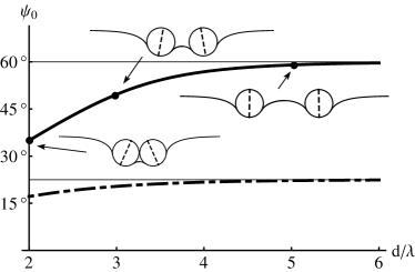
Figure 4: (a) Inner contact angle $\psi_{0}$ and (b) derivative of the arc length $\partial s_{0}/\partial d$ as a function of $d/\lambda$ for $R/\lambda=1$ and $\alpha_{\text{c}}=45^{\circ}$ (dashed-dotted line) and $120^{\circ}$ (solid line). The thin solid lines correspond to the respective large $d$ limits.

The curve of $-F^{\text{fl}}$ shows two characteristic trends: at short separations $d/\lambda\approx 2,$ the force increases with $d$. This is due to a fast rotation of the cylinders for an infinitesimal change in $d$ (see Fig. 4) which implies that the length $2s_{0}$ of the inner membrane stays almost unchanged, i. e., $\partial s_{0}/\partial d$ is small. The membrane is thus more under tension and thermal fluctuations are strongly reduced. Since $\partial s_{0}/\partial d$ increases with $d$, the force grows until it reaches a maximum value at $\partial s_{0}/\partial d\approx 1/2$. For larger separations, $\psi_{0}$ and $\partial s_{0}/\partial d$ stay constant and the force $-F_{\text{in}}^{\text{fl}}$ should decrease in a monotonous manner until it tends to the constant value $L\Lambda^{2}/(2\pi^{2}\beta)$ in the limit $d/\lambda\rightarrow\infty$. Actually, this monotonous decrease of the force—expected on physical grounds—can be exploited to fix the fitting parameter $\delta$: as shown in Fig. 5, $\delta$ has to be set to a value smaller than $10^{-6}$.

\psfrag{Ftin}{$-\tilde{F}_{\text{in}}^{\text{fl}}/L$}\psfrag{A}{$\delta=10^{-1}$}\psfrag{B}{$\delta=10^{-2}$}\psfrag{C}{$\delta=10^{-3}$}\psfrag{D}{$\delta\leq 10^{-6}$}\includegraphics*[width=195.12767pt]{fig5.eps}

Figure 5: Scaled thermal force $-\tilde{F}_{\text{in}}^{\text{fl}}/L:=-2\pi\beta F_{\text{in}}^{\text{fl}}/(L\Lambda^{2})$ on the left cylinder as a function of separation $d/\lambda\geq 2$ for $R/\lambda=1$, $\alpha_{\text{c}}=120^{\circ}$ and fitting parameters $\delta=10^{-1},10^{-2},10^{-3}$, and $\leq 10^{-6}$. The first three curves reach the limit $1/\pi$ at $d/\lambda\rightarrow\infty$ from below. All curves with $\delta\leq 10^{-6}$ are identical for the given resolution of the figure and give a monotous unique force.

To summarize, the total force per length $F_{\text{cyl}}/L=(F_{\text{cyl}}^{(0)}+F^{\text{fl}})/L$ on the left cylinder is

$$F_{\text{cyl}}/L=-\sigma(1-\eta)+F_{\text{in}}^{\text{fl}}/L+\Lambda^{2}/(2\pi^{2}\beta)\;.$$ (24)

Since this force is always negative, there is no equilibrium position beside the limit $d/\lambda\rightarrow\infty$, where $F_{\text{cyl}}\rightarrow 0$.

IV Conclusion

By developing a new approach for the computation of the free energy for a system of two cylinders bound on the same side of a membrane, we could evaluate the corrections caused by the thermal fluctuations to the repelling zero temperature force. It was found that this contribution in the section between the cylinders strongly depends on the membrane curvature. The calculated thermal force is always repulsive. This effect differs from the attractive Casimir force which arises from the reduction of the number of internal modes with respect to the outer ones where the ground state is identical everywhere. This is obviously not the case here since the zero temperature shapes of the inner and outer sections are different: even though the number of modes in the inner section is smaller than in the outer ones, their fluctuations are strongly enhanced on a curved background and thus always dominate the fluctuations of the outer less curved region. Non-trivial membrane geometries as the one presented here are in fact ubiquitous in nature. The approach of this paper is sufficiently general to calculate the physical properties of other systems with highly curved ground states.

This research was supported in part by the National Science Foundation under Grant No. NSF PHY05-51164.

Appendix A Derivation of the fluctuation operator $H^{(2)}$ (see Eq. (5))

To rewrite the Helfrich Hamiltonian (1) in terms of the parametrization ${\bm{X}}(s,y)$, one has to replace the area element ${\text{d}}A$ and the curvature $K$ in (1) using the functions $u(s,y)$, $\psi(s)$, and their derivatives DifferentialGeometry . First, one needs to determine the components of the (symmetric) metric tensor $g_{ab}$ ($a,b\in\{s,y\}$) :

$$g_{ss} = \left(\frac{\partial{\bm{X}}}{\partial s}\right)^{2}=(u\dot{\psi}-1)^{2}+u_{s}^{2}\;,$$

$$g_{sy}\textasciiacute = \frac{\partial{\bm{X}}}{\partial y}\cdot\frac{\partial{\bm{X}}}{\partial s}=u_{y}u_{s}\;,\quad\text{and}$$

$$g_{yy} = \left(\frac{\partial{\bm{X}}}{\partial y}\right)^{2}=1+u_{y}^{2}\;,$$ (25)

where we have introduced the notations $\dot{\psi}\equiv\partial\psi/\partial s$, $u_{s}\equiv\partial u/\partial s$ and $u_{y}\equiv\partial u/\partial y$. This allows to calculate the area element ${\text{d}}A=\sqrt{g}\,{\text{d}}s{\text{d}}y$ with $\sqrt{g}=\sqrt{\det{(g_{ab})}}=\sqrt{(u\dot{\psi}-1)^{2}(1+u_{y}^{2})+u_{s}^{2}}$. The components of the extrinsic curvature tensor $K_{ab}$ are:

$$K_{ss} = \frac{\partial{\bm{X}}}{\partial s}\cdot\frac{\partial{\bm{n}}}{\partial s}=\frac{1}{\sqrt{g}}\left[-\dot{\psi}+2u\dot{\psi}^{2}-u_{ss}-u^{2}\dot{\psi}^{3}-uu_{s}\ddot{\psi}+(uu_{ss}-2u_{s}^{2})\,\dot{\psi}\right]$$

$$K_{sy} = \frac{\partial{\bm{X}}}{\partial y}\cdot\frac{\partial{\bm{n}}}{\partial s}=\frac{1}{\sqrt{g}}\left[(-1+u\dot{\psi})\,u_{sy}-\dot{\psi}u_{y}u_{s}\right]\;,\quad\text{and}$$

$$K_{yy} = \frac{\partial{\bm{X}}}{\partial y}\cdot\frac{\partial{\bm{n}}}{\partial y}=\frac{1}{\sqrt{g}}(-1+u\dot{\psi})\,u_{ss}\;.$$ (26)

The contraction of $K_{ab}$ with the metric yields the curvature $K=\sum K_{ab}g^{ab}$ where $g^{ab}$ is the inverse of the metric, $i.e.$, $g^{ss}=g_{yy}/g$, $g^{sy}=-g_{sy}/g$, and $g^{yy}=g_{ss}/g$. Inserting the expressions for ${\text{d}}A$ and $K$ into $H$ one identifies

$$H^{(2)} =\int[\frac{\dot{\psi}^{4}u^{2}}{2}+\dot{\psi}\ddot{\psi}u_{s}u+(\frac{1}{\lambda^{2}}+\frac{3\dot{\psi}^{2}}{2})\frac{u_{s}^{2}}{2}+\dot{\psi}^{2}u_{ss}u$$ (27)

$$+\frac{u_{ss}^{2}+u_{yy}^{2}}{2}+u_{ss}u_{yy}+(\frac{1}{\lambda^{2}}-\frac{\dot{\psi}^{2}}{2})\frac{u_{y}^{2}}{2}]\text{d}s\text{d}y\;.$$

Appendix B Derivation of Eq. (15)

Let $X(0)={\text{{X}}}(0,0,0)$ and start with expression (14)

$$\beta\delta F=\frac{1}{2}\sum_{q}\frac{\frac{\partial}{\partial d}\sum_{n}X(0)\tilde{{\text{{G}}}}(n,q)}{1+\sum_{n}X(0)\tilde{{\text{{G}}}}(n,q)}\;.$$ (28)

Note that, according to their definition, $\frac{\partial}{\partial d}X(0)=-\frac{1}{d}X(0)$ and $\frac{\partial}{\partial d}\sum_{n}\tilde{{\text{{G}}}}(n,q)=\frac{2}{d}\sum_{n}\frac{\lambda^{2}\left(\frac{2\pi n}{d}\right)^{2}}{\left[\left(\frac{2\pi n}{d}\right)^{2}+\left(\frac{2\pi q}{L}\right)^{2}\right]^{2}}$. Thus, a continuous approximation for the sum (which is valid for large $d$, given the high number of modes) yields for large separations:

$$\frac{\partial}{\partial d}\sum_{n}X(0)\tilde{{\text{{G}}}}(n,q) =-\frac{X(0)}{\pi}\lambda^{2}\int_{\frac{2\pi}{d}}^{\Lambda}\left[\frac{1}{\left(n^{2}+q^{2}\right)}-\frac{2n^{2}}{\left(n^{2}+q^{2}\right)^{2}}\right]{\text{d}}n$$

$$\simeq-\frac{X(0)}{\pi}\lambda^{2}\Lambda\frac{q^{2}-\frac{2\pi}{d}\Lambda}{\left(\Lambda^{2}+q^{2}\right)\left[\left(\frac{2\pi}{d}\right)^{2}+q^{2}\right]}$$

and by the same token:

$$1+\sum_{n}X(0)\tilde{{\text{{G}}}}(n,q)=1+\frac{\lambda^{2}}{\pi}X(0)d\int_{\frac{2\pi}{d}}^{\Lambda}\frac{1}{n^{2}+q^{2}}\,{\text{d}}n\simeq 1+\frac{\lambda^{2}}{\pi}\frac{X(0)d}{q}\arctan\left(\frac{q}{\frac{2\pi}{d}+\frac{q^{2}}{\Lambda}}\right)\,.$$

As a consequence Eq. (28) becomes in the continuum approximation:

$$\beta\delta F=-\frac{1}{d}\frac{L}{2\pi}\int_{\frac{2\pi}{d}}^{\Lambda}\frac{\frac{X\left(0\right)d}{\pi}\lambda^{2}\Lambda\frac{q^{2}-\frac{2\pi}{d}\Lambda}{\left(\Lambda^{2}+q^{2}\right)\left[\left(\frac{2\pi}{d}\right)^{2}+q^{2}\right]}}{1+\frac{\lambda^{2}}{\pi}\frac{X(0)d}{q}\arctan\left(\frac{q}{\frac{2\pi}{d}+\frac{q^{2}}{\Lambda}}\right)}{\text{d}}q\;.$$

A careful inspection of this expression can be performed by dividing the integration interval into three parts, $\left[\frac{2\pi}{d},\sqrt{\frac{2\pi}{d}\Lambda}\right],$ $\left[\sqrt{\frac{2\pi}{d}\Lambda},\left(\frac{2\pi}{d}\Lambda^{3}\right)^{\frac{1}{4}}\right]$ and $\left[\left(\frac{2\pi}{d}\Lambda^{3}\right)^{\frac{1}{4}},\Lambda\right]$. It turns out that the contributions of the two first intervals are negligible with respect to the last one. Moreover, checking that in the range of integration considered, the numerator $q^{2}-\frac{2\pi}{d}\Lambda$ can be approximated by $q^{2}$, we can thus write $\beta\delta F$ for large $d$ as:

$$\beta\delta F\simeq-\frac{1}{d}\frac{L}{2\pi}\int_{0}^{\Lambda}\frac{\frac{X\left(0\right)d}{\pi}\lambda^{2}\Lambda\frac{1}{\left(\Lambda^{2}+q^{2}\right)}}{1+\frac{\lambda^{2}}{\pi}\frac{X\left(0\right)d}{q}\arctan\left(\frac{\Lambda}{q}\right)}{\text{d}}q\;.$$ (29)

Ultimatly, the evaluation of $\beta\delta F$ requires the computation of

$$X(0)={\text{{X}}}(0,0,0)=\frac{1}{d}\int_{-\frac{d}{2}}^{\frac{d}{2}}\left[\frac{1}{2}\dot{\psi}^{4}+\frac{3}{2}\left(\ddot{\psi}^{2}+\frac{1}{\lambda^{2}}\dot{\psi}^{2}\right)\right]{\text{d}}s\;.$$ (30)

This computation relies on the saddle point solution $\psi(s)$. Actually, for large $d$, $\eta\simeq 1$ one has

$$\dot{\psi}\simeq\sqrt{2\left(\frac{1-\cos\left(\psi\right)}{\lambda^{2}}\right)}=\frac{2}{\lambda}\left|\sin\left(\frac{\psi}{2}\right)\right|$$

whose solution is:

$$\psi(s)=2\arccos\left[\frac{1-C\exp\big{(}2\frac{s-s_{0}}{\lambda}\big{)}}{1+C\exp{\big{(}2\frac{s-s_{0}}{\lambda}\big{)}}}\right]$$

with $C=\tan^{2}\left(\frac{\psi_{0}}{4}\right)$. As a consequence, replacing $\psi(s)$ in Eq. (30) one finds directly that $X(0)=\frac{16}{3}C\frac{\left(2C+3\right)\left(5C+3\right)}{d\lambda^{3}\left(C+1\right)^{3}}$. Inserting this value in the expression of $\beta\delta F$ in Eq. (29) leads to the result claimed in the text.

References

- (1) H. B. G. Casimir, Proc. K. Ned. Akad. Wet. 51, 793 (1948).
- (2) M. E. Fisher and P. G. de Gennes, C. R. Seances Acad. Sci., Ser. B 287, 207 (1978).
- (3) C. Hertlein et al., Nature 451, 172 (2008).
- (4) M. Kresch, The Casimir Effect in Critical Systems (World Scientific, Singapore) 1994.
- (5) H. Li and M. Kardar, Phys. Rev. Lett. 67, 3275 (1991).
- (6) H. Lehle, M. Oettel, and S. Dietrich, Europhys. Lett. 75, 174 (2006).
- (7) E. Noruzifar and M. Oettel, Phys. Rev. E 79, 051401 (2009).
- (8) B. J. Reynwar et al., Nature 447, 461 (2007).
- (9) M. Goulian, R. Bruinsma, and P. Pincus, Europhys. Lett. 22, 145 (1993); ibid. 23, 155(E) (1993).
- (10) R. Golestanian, M. Goulian, and M. Kardar, Europhys. Lett. 33, 241 (1996); Phys. Rev. E 54, 6725 (1996).
- (11) J.-M. Park and T. C. Lubensky, J. Phys. I France 6, 1217 (1996).
- (12) K. S. Kim, J. C. Neu, and G. F. Oster, Europhys. Lett. 48, 99 (1997).
- (13) P. G. Dommersnes and J.-B. Fournier, Europhys. Lett. 46, 256 (1999).
- (14) T. R. Weikl, Eur. Phys. J. E 12, 265 (2003).
- (15) C. Yolcu, I. Z. Rothstein, and M. Deserno, arXiv:1007.4760v1.
- (16) H.-K. Lin, R. Zandi, U. Mohideen, and L. P. Pryadko, arXiv:1009.0724v1.
- (17) P. Biscari, F. Bisi, and R. Rosso, J. Math. Biol. 45, 37 (2002); P. Biscari and F. Bisi, Eur. Phys. J. E 7, 381 (2002). P. Biscari and G. Napoli, Biomechan. Model Mechanobiol. 6, 297 (2007).
- (18) M. M. Müller, M. Deserno, and J. Guven, Europhys. Lett. 69, 482 (2005); Phys. Rev. E 72, 061407 (2005).
- (19) M. M. Müller, M. Deserno, and J. Guven, Phys. Rev. E 76, 011921 (2007).
- (20) S. Mkrtchyan, C. Ing, and J. Z. Y. Chen, Phys. Rev. E 81, 011904 (2010).
- (21) P. B. Canham, J. Theoret. Biol. 26, 61 (1970).
- (22) W. Helfrich, Z. Naturforsch. 28c, 693 (1973).
- (23) For a detailed introduction to the differential geometry of two-dimensional surfaces see: M. Do Carmo, Differential Geometry of Curves and Surfaces, (Prentice Hall, 1976); E. Kreyszig, Differential Geometry, (Dover, New York 1991).
- (24) J.-B. Fournier and C. Barbetta, Phys. Rev. Lett. 100, 078103 (2008).
- (25) R. Capovilla, J. Guven, and J. A. Santiago, J. Phys. A: Math. and Gen. 36, 6281 (2003).
- (26) The Jacobian is an infinite constant that does not affect the physical quantities and can thus be disregarded.
- (27) Handbook of Mathematical Functions, 9th ed., ed. by M. Abramowitz and I. A. Stegun (Dover, New York, 1970).
- (28) J.-B. Fournier and P. Galatola, Phys. Rev. Lett. 98, 018103 (2007).