Alpha effect due to buoyancy instability of a magnetic layer

Abstract

Context. A strong toroidal field can exist in form of a magnetic layer in the overshoot region below the solar convection zone. This motivates a more detailed study of the magnetic buoyancy instability with rotation.

Aims. We calculate the $\alpha$ effect due to helical motions caused by a disintegrating magnetic layer in a rotating density-stratified system with angular velocity $\Omega$ making an angle $\theta$ with the vertical. We also study the dependence of the $\alpha$ effect on $\theta$ and the strength of the initial magnetic field.

Methods. We carry out three-dimensional hydromagnetic simulations in Cartesian geometry. A turbulent EMF due to the correlations of the small scale velocity and magnetic field is generated. We use the test-field method to calculate the transport coefficients of the inhomogeneous turbulence produced by the layer.

Results. We show that the growth rate of the instability and the twist of the magnetic field vary monotonically with the ratio of thermal conductivity to magnetic diffusivity. The resulting $\alpha$ effect is inhomogeneous and increases with the strength of the initial magnetic field. It is thus an example of an “anti-quenched” $\alpha$ effect. The $\alpha$ effect is nonlocal, requiring around 8–16 Fourier modes to reconstruct the actual EMF based on the actual mean field.

1 Introduction

The magnetic fields in many astrophysical bodies have their origin in some kind of turbulent dynamo. This means that a part of the kinetic energy of the turbulent motions is diverted to enhancing and maintaining a magnetic field. This magnetic field is generally also random, but under certain conditions a large-scale magnetic field can also emerge. Here by large-scale we mean length scales larger than the energy containing scale of the fluid. This can be the case when the turbulence is helical, e.g., owing to the simultaneous presence of rotation and stratification.

The evolution of the large-scale magnetic field can be described using averaged evolution equations. In the process of averaging, new terms emerge (e.g., the $\alpha$ effect and turbulent diffusion) that result from correlations between small-scale velocity and magnetic fields. Here one usually considers the case where the magnetic fluctuations are caused by the fluctuating velocity acting on the mean field. However, under certain conditions it might well be the other way around. Imagine, for example, the case where initially no velocity is present, but there is instead a strong large-scale magnetic field the presence of which makes the initial state of zero velocity unstable. In that case the magnetic field would be responsible for driving velocity and magnetic fluctuations at the same time. This type of scenario was first simulated in the context of accretion discs where the magneto-rotational instability drives turbulence (Brandenburg et al., 1995), and later in the context of the magnetic buoyancy instability with shear (Cline et al., 2003), which might apply to the overshoot layer of the Sun. It had already been proposed by Moffatt (1978) that, once the dynamo-generated magnetic field in this layer reaches appreciable strengths, the magnetic buoyancy instability can set in and govern the dynamics thereafter. The linear phase of this instability in a localized flux layer with stratification and rotation was later studied in detail by Schmitt (1984, 1985). A necessary but not sufficient condition for this instability is

$$\frac{\partial}{\partial z}\log\left(\frac{B}{\rho}\right)<0,$$ (1)

which essentially means that the magnetic field modulus $B$ decreases faster with height $z$ than the density $\rho$. Brandenburg & Schmitt (1998) performed numerical calculations in presence of rotation and determined the $\alpha$ effect of the resulting turbulence by imposing an external magnetic field.

This type of magnetic buoyancy instability is also related to the undulatory instability in the absence of both rotation and shear (Fan, 2001) and the double diffusive instability (Silvers et al., 2009) in presence of shear and no rotation. While the focus of the first study has been on the formation of flux tubes from a pre-existing toroidal magnetic layer in a stably stratified atmosphere, in the latter a magnetic layer was generated from an initially vertical magnetic field in presence of strong shear. It was further shown that, when the ratio of magnetic to thermal diffusivities is sufficiently low, magnetic buoyancy can still operate in the tachocline.

The focus of this work is twofold. Firstly, we want to study the nature of the instability at short times, i.e., in its initial linear stage. In particular, its dependence on various parameters such as magnetic and thermal Prandtl numbers, angular velocity, strength of the initial field, etc, and compare against the linear theory and previous numerical work. It can be argued that in presence of rotation this instability produces magnetostrophic waves due to balance between Coriolis and Lorentz forces. An important result highlighted later is that rotation is not vital to the growth of this instability. Secondly, we want to study whether this instability constitutes a viable dynamo process, so we want to measure the mean-field transport coefficients, namely the tensors $\alpha$ and $\eta$ using the quasi-kinematic test-field (QKTF) method (Schrinner et al., 2005, 2007). However, with one exception (Vermersch & Brandenburg, 2009), the QKTF has never been applied to the calculation of transport coefficients in an inhomogeneous turbulence induced by the mean magnetic field itself. Therefore we aim to first verify the applicability of the QKTF method to this problem. For a review on transport coefficients and their determination using test fields; see Brandenburg et al. (2010). The applicability of this method to problems with an initial magnetic field and fluctuations generated from it is discussed in Rheinhardt & Brandenburg (2010).

2 The Model

We consider a setup similar to that described in Brandenburg & Schmitt (1998). The computational domain is a cuboid with constant gravity, $g_{z}$, pointing in the negative $z$ direction, and rotation $\boldsymbol{\Omega}$ making an angle $\theta$ with the vertical. The box may be thought to be placed at a colatitude $\theta$ on the surface of a sphere with its unit vectors $\boldsymbol{\hat{x}},\boldsymbol{\hat{y}},\boldsymbol{\hat{z}}$ pointing along the local $\theta,\,\phi,\,r$ directions, respectively, as shown in Fig. 1.

We solve the following set of MHD equations. The continuity equation is given by

$$\frac{\mathrm{D}\ln\rho}{\mathrm{D}t}=-\mbox{\boldmath{$\nabla$}}\cdot\mbox{\boldmath$U$}{},$$ (2)

where $\mathrm{D}/\mathrm{D}t\equiv\partial/\partial t+\mbox{\boldmath$U$}{}\cdot\mbox{\boldmath$\nabla$}{}$ denotes the Lagrangian derivative with respect to the local velocity of the gas $U$. Assuming an ideal gas, we express the pressure in terms of density, specific entropy $s$, and sound speed $c_{\rm s}$, which, in turn, is a function of $\rho$ and $s$. Thus the momentum equation in a frame of reference rotating with angular velocity $\boldsymbol{\Omega}$ reads

$$\frac{\mathrm{D}\mbox{\boldmath$U$}{}}{\mathrm{D}t}= -c_{\rm s}^{2}\mbox{\boldmath$\nabla$}{}\biggl{(}\frac{s}{c_{p}}+\ln\rho\biggr{)}-2\boldsymbol{\Omega}\times\mbox{\boldmath$U$}{}+g_{z}\mbox{\boldmath{$\hat{z}$}}+\frac{\mbox{\boldmath$J$}{}\times\mbox{\boldmath{$B$}}}{\rho}$$ (3)

$$+\nu\left(\nabla^{2}\mbox{\boldmath$U$}{}+\frac{1}{3}\mbox{\boldmath$\nabla$}{}\mbox{\boldmath{$\nabla$}}\cdot\mbox{\boldmath$U$}{}+2\mbox{\boldmath${\sf S}$}{}\cdot\mbox{\boldmath$\nabla$}{}\ln\rho\right),$$

where $J$ is the current density, $B$ is the magnetic field, $\nu$ is the constant kinematic viscosity, and ${\sf S}$ is the traceless rate-of-strain tensor. The sound speed is related to temperature by $c_{\rm s}^{2}=(c_{p}-c_{v})\gamma T$ with $c_{p}$ and $c_{v}$ the specific heat at constant pressure and constant volume, respectively, and $\gamma=c_{p}/c_{v}$ is here fixed to $5/3$. The induction equation is solved in terms of the magnetic vector potential $A$, such that $\mbox{\boldmath$\nabla$}{}\times\mbox{\boldmath{$A$}}=\mbox{\boldmath{$B$}}$, hence

$$\frac{\partial\mbox{\boldmath{$A$}}}{\partial t}=\mbox{\boldmath$U$}{}\times\mbox{\boldmath{$B$}}+\eta\nabla^{2}\mbox{\boldmath{$A$}}\,,\\$$ (4)

where $\eta$ denotes constant molecular magnetic diffusivity.

Finally, we have for the entropy equation with temperature $T$ and constant radiative (thermal) conductivity $K$

$$\rho T\frac{\mathrm{D}s}{\mathrm{D}t}=\mbox{\boldmath{$\nabla$}}\cdot(K\mbox{\boldmath$\nabla$}{}T)+\eta\mu_{0}\mbox{\boldmath$J$}{}^{2}+2\rho\nu\mbox{\boldmath${\sf S}$}{}^{2}\,,$$ (5)

where the temperature is related to the specific entropy by

$$s=s_{0}+c_{v}\ln\frac{T/T_{0}}{(\rho/\rho_{0})^{\gamma-1}}\,.$$ (6)

We use the fully compressible Pencil Code for all our calculations.

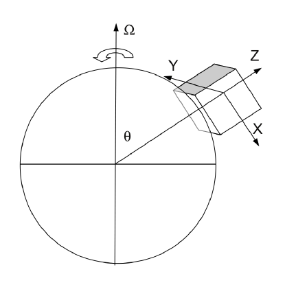
Figure 1: The Cartesian simulation domain with respect to spherical coordinates.

For all quantities, periodic boundary conditions in the $x$ and $y$ directions are adopted. In the $z$ direction we use the no-slip boundary condition for the velocity, the vertical field condition for the magnetic field, as a proxy for vacuum boundaries. We keep the temperature at the top and the (radiative) heat flux at the bottom fixed. Their values were chosen to conform with the initial temperature profile of the (not magnetically modified) polytrope described below.

2.1 Initial state

The base state is a polytrope that is, $p=C\rho^{\Gamma}$, with index $m=1/(\Gamma-1)=3$. The initial $z$ profiles of density, pressure, temperature and entropy are given by,

$$\rho_{i} =\rho_{0}\Phi^{3}(z),\quad p_{i}=p_{0}\Phi^{4}(z),\quad T_{i}=T_{0}\Phi(z),$$ (7)

$$s_{i} =s_{0}-c_{v}\ln\Phi(z),$$

where $\Phi$ is a non-dimensional gravitational potential given by

$$\Phi(z)=1+\frac{1}{4}\frac{g_{z}}{T_{0}(c_{p}-c_{v})}(z-z_{0}),$$

with the reference point $z_{0}$ chosen to be at the bottom of the domain and the values at this point given by $\rho_{0}$, $p_{0}=c_{s0}^{2}\rho_{0}/\gamma$, $T_{0}=c_{s0}^{2}/(c_{p}-c_{v})\gamma$ and $s_{0}$. Here $c_{\rm s0}$ is the reference sound speed to which we also refer to when calculating Mach numbers.

As the adiabatic index is here $m_{\rm ad}=1/(\gamma-1)=3/2$, the subadiabaticity in the domain is very large, namely $\partial\ln T/\partial\ln P-(\partial\ln T/\partial\ln P)_{\rm ad}=-0.15$. Thus, the initial stratification is highly stable to convection in the absence of any magnetic field, guaranteeing that turbulence is generated solely by the buoyancy instability.

The initial magnetic field is a horizontal layer of thickness $H_{B}$, where $B_{y}$ has the profile

$$B_{y0}=B_{0}H_{\rm B}\frac{\partial{}}{\partial\hskip 0.59998pt{z}}\tanh\left(\frac{z-z_{B}}{H_{\rm B}}\right),$$ (8)

and the reference Alfvén speed is defined by $v_{\rm A0}=B_{0}/\sqrt{\rho_{0}\mu_{0}}$ with $\mu_{0}$ being the vacuum permeability. If not indicated otherwise, the initial magnetic field strength is fixed to $v_{\rm A0}/c_{\rm s0}=0.5$. In order to satisfy the condition (1) initially, we have to ensure $H_{B}<H_{\rho}(z_{B})$, where $H_{\rho}(z)=|\mbox{\boldmath$\nabla$}{}\ln\rho(z)|^{-1}$ is the local density scale height. When choosing $z_{B}-z_{0}=0.3L_{z}$ this is satisfied for $H_{B}<0.1L_{z}+4T_{0}(c_{p}-c_{v})/3|g_{z}|$ which is surely true for the choice $H_{B}=0.05L_{z}$.

Upon addition of a magnetic field, we have to modify the base state such that the density profile remains unchanged. In order to obey magnetostatic equilibrium, pressure and temperature are adjusted in the following way:

$$p_{i}\Rightarrow p_{i}-\frac{B_{y0}^{2}}{2\mu_{0}},\qquad T_{i}\Rightarrow T_{i}-\frac{B_{y0}^{2}}{2\mu_{0}}\frac{1}{\rho_{i}(c_{p}-c_{v})}.$$ (9)

The entropy is then re-calculated from Eq. (6). The initial velocity components $U_{x}$ and $U_{y}$ are specified such that it contains about 20 localized eddies in the plane $z=z_{B}$ with Mach numbers of about $10^{-5}$. Also the initial vertical velocity, $U_{z}$ is Gaussian random noise with the same Mach number. The rms of the initial kinetic helicity, scaled with the product of initial rms velocity and vorticity, is denoted $\varepsilon_{\rm K0}$, that is, $\varepsilon_{\rm K0}=(\sqrt{\langle(\boldsymbol{W}\cdot\boldsymbol{U})^{2}\rangle}/U_{\mathrm{rms}}W_{\mathrm{rms}})(0)=4\times 10^{-6}$.

2.2 Control parameters, nondimensional quantities, and computational grid

The problem posed by (2) through (5) is governed by five independent dimensionless parameters, (i) the Prandtl number $\Pr=\nu/\chi_{0}$, with the temperature conductivity $\chi_{0}=K/\rho_{0}c_{p}$, (ii) the magnetic Prandtl number $\mbox{\rm Pr}_{\rm M}=\nu/\eta$, (iii) the “magnetic Taylor number” ${\mathrm{Ta}_{\mathrm{M}}}=2\Omega^{2}L_{y}^{4}/\eta^{2}$, (iv) the rotational inclination (colatitude), $\theta$, and (v) the normalized gravitational acceleration $g_{z}L_{y}^{3}\eta^{2}$. In addition there are two independent parameters of the initial equilibrium (vi) the normalized pressure scale height at the bottom, $H_{P}/L_{z}=c_{s0}^{2}/\gamma g_{z}L_{z}$ and (vii) the initial Lundquist number, $\mbox{\rm Lu}_{0}=v_{\rm A0}H_{B}/\eta$, based upon the thickness of the magnetic layer. In addition to this, we also have the non-dimensional sound speed, $c_{s0}L_{y}/\eta$. In this paper we shall keep the normalized pressure scale height and the sound speed fixed, while varying both Prandtl numbers, ${\mathrm{Ta}_{\mathrm{M}}}$, $\theta$ and $\mbox{\rm Lu}_{0}$. The definitions as well as the values or ranges of the control parameters are summarized in Table 1. We have also included in the same table two dependent parameters namely the modified initial plasma-beta in the midplane of the magnetic layer and the Roberts number $\mathrm{Rb}=\mbox{\rm Pr}_{\rm M}/\Pr=\chi_{0}/\eta$.

The computational domain is defined by $|x|\leq L_{x}/2$, $|y|\leq L_{y}/2$, $-L_{z}/4\leq z\leq 3L_{z}/4$, $L_{x}=L_{z}=L_{y}/3$, thus its aspect ratio is 1:3:1. The results will be presented in non-dimensional form, velocity in units of the reference Alfvén speed, $v_{\mathrm{A}0}$, time in units of the corresponding Alfvén travel time in the $y$ direction, $t_{\rm A0}=L_{y}/v_{\mathrm{A}0}$, and magnetic field in units of $B_{0}$ or the rms value $(\int_{z}B_{y0}^{2}{\rm d}{}z/L_{z})^{1/2}$.

It is instructive to look upon the relevant definitions of the fluid Reynolds number, Re, and the magnetic Reynolds number, $\mbox{\rm Re}_{\rm M}$, for this problem where the turbulence is driven solely by the instability of the magnetic layer. From first principles, the Re characterizes the ratio of the advective term $\langle\boldsymbol{(U\cdot\nabla U})^{2}\rangle^{1/2}$ and the viscous term $\langle(\nu\nabla^{2}\boldsymbol{U})^{2}\rangle^{1/2}$ in the Navier-Stokes equation, while $\mbox{\rm Re}_{\rm M}$ characterizes the ratio of $\langle\big{(}\boldsymbol{\nabla}\times(\boldsymbol{U}\times\boldsymbol{B})\big{)}^{2}\rangle^{1/2}$ and $\langle(\eta\nabla^{2}\boldsymbol{B})^{2}\rangle^{1/2}$ in the induction equation with the angular brackets representing volume averaging. Let us denote these ab initio definitions as “term-based” and refer to them by $\mbox{\rm Re}^{*}$ and $\mbox{\rm Re}_{\rm M}^{*}$. Note, that with the term-based definitions $\mbox{\rm Re}_{\rm M}/\mbox{\rm Re}$ may well deviate from $\mbox{\rm Pr}_{\rm M}$. Alternatively, we can define a length scale $L_{U}=U_{\rm rms}/2\pi W_{\rm rms}$ from the rms values of velocity and vorticity and define the more conventional “length-based” Reynolds numbers $\mbox{\rm Re}=U_{\mathrm{rms}}L_{U}/\nu$ and $\mbox{\rm Re}_{\rm M}=U_{\mathrm{rms}}L_{U}/\eta$.

The calculations were carried out on equidistant grids with resolutions of either $64^{3}$ or $128^{3}$. For numerical testing we have also performed a few runs with $256^{3}$ or $128^{2}\times 256$ resolutions.

Table 1: Non-dimensional control parameters characterizing the buoyancy instability. Note the definition of the modified plasma-beta $\,\hskip 0.85358pt\widetilde{\!\beta}$ as the ratio of the total pressure $p_{\mathrm{tot}}=p+p_{\mathrm{M}}$ to the magnetic pressure $p_{\mathrm{M}}=B_{y0}^{2}/2\mu_{0}$, because this quantity adopts a simple $1/B^{2}$ dependence on the magnetic field, cf Eq. (9). Values of $\,\hskip 0.85358pt\widetilde{\!\beta}$ refer to $t=0$ and the midplane of the magnetic sheet.

Parameter	Symbol	Definition	Value/Range
norm. scale height		$H_{P}/L_{z}$	0.3
norm. sound speed		$c_{s0}L_{y}/\eta$	$6\times 10^{4}$
Prandtl number	$\rm Pr$	$\nu/\chi_{0}$	0.125 …4.0
magnetic Prandtl no.​​	$\rm Pr_{\rm M}$	$\nu/\eta$	0.125 …4.0
Roberts number	$\rm Rb$	$\chi_{0}/\eta$	0.25 …1.0
magnetic Taylor no.	${\mathrm{Ta}_{\mathrm{M}}}$	$\Omega^{2}L_{\rm y}^{4}/\eta^{2}$	$0\ldots 3.2\times 10^{10}$
rotational inclination	$\theta$	$\varangle(\boldsymbol{\Omega},\,\hskip 0.85358pt\hat{\!\mbox{\boldmath$z$}{}})$	0 …180
(initial) Lundquist no.	$\rm Lu_{0}$	$v_{\rm A0}H_{\rm B}/\eta$	500 …600
(initial) modified	$\,\hskip 0.85358pt\widetilde{\!\beta}_{0}$	$(p_{\mathrm{tot}}/p_{\mathrm{M}})(z_{\rm B},0)$	1.04 …3.22
plasma-beta

2.3 The test-field method

Table 2: List of runs of set B. The computational box is placed at colatitude $\theta=30^{\circ}$. Magnetic Taylor number ${\mathrm{Ta}_{\mathrm{M}}}=3.24\times 10^{10}$, initial Lundquist number $\mbox{\rm Lu}_{0}=500$, initial plasma-beta $\,\hskip 0.85358pt\widetilde{\!\beta}_{0}=2.27$ and resolution $128^{3}$ throughout. $\rm Ma$ – Mach number, based on $U_{\mathrm{rms}}$, $\omega_{\mathrm{I}}$ – growth rate. Saturation reached at $t^{\rm sat}$. For the mean EMF in the saturated stage global extrema of the dominating ${\cal E}^{\rm sat}_{y}$ with respect to $z$ and $t$ are given.

Run	$\Pr$	$\mbox{\rm Pr}_{\rm M}$	$\rm Ma$	$\omega_{\mathrm{I}}\,t_{\rm A0}$	$t^{\rm sat}/t_{\rm A0}$	$10^{4}\times{\cal E}_{y}^{\rm sat}/v_{\rm A0}B_{0}$		length-based	term-based
						min	max	$\mbox{\rm Re}\,(L_{U})$	$\mbox{\rm Re}^{*}$	$\mbox{\rm Re}_{\rm M}^{*}$	$\mbox{\rm Re}_{\rm M}^{*}/\mbox{\rm Re}^{*}$
B128a	4.0	4.0	0.017	15.6	1.99	$-1.01$	2.34	0.5	0.4	2.3	5.8
B128b	1.0	4.0	0.036	21.6	1.42	$-3.39$	7.32	0.9	0.6	2.8	4.5
B128c	1.0	1.0	0.020	13.2	1.64	$-1.49$	3.03	1.8	1.4	1.9	1.4
B128d	0.25	1.0	0.038	25.2	1.27	$-4.02$	7.52	2.9	2.1	2.8	1.3
B128e	0.125	0.5	0.036	24.0	1.22	$-5.47$	6.19	3.6	3.3	2.9	0.9
B128f	0.125	0.125	0.043	19.9	1.54	$-3.50$	4.84	8.2	16.1	3.1	0.2
B128g	0.5	0.5	0.018	19.2	1.72	$-2.06$	3.69	2.9	2.5	1.9	0.8
B128h	0.5	1.0	0.032	21.6	1.67	$-3.94$	3.97	1.7	1.9	3.2	1.7

We now define mean magnetic and velocity fields, $\overline{\mbox{\boldmath$B$}}{}$ and $\overline{\mbox{\boldmath$U$}}$, where overbars denote horizontal averaging. Fluctuations are defined correspondingly as $\mbox{\boldmath$b$}{}=\mbox{\boldmath$B$}{}-\overline{\mbox{\boldmath$B$}}{}$ and $\mbox{\boldmath$u$}{}=\mbox{\boldmath$U$}{}-\overline{\mbox{\boldmath$U$}}$. Following the above convention, the induction equation may be horizontally averaged as,

$$\frac{\partial{\overline{\mbox{\boldmath$B$}}{}}}{\partial\hskip 0.59998pt{t}}=\mbox{\boldmath$\nabla$}{}\times\left(\overline{\mbox{\boldmath$U$}}\times\overline{\mbox{\boldmath$B$}}{}\right)+\mbox{\boldmath$\nabla$}{}\times\overline{\mbox{\boldmath${\cal E}$}}{}+\eta\nabla^{2}\overline{\mbox{\boldmath$B$}}{},$$ (10)

where $\eta$ is the molecular magnetic diffusivity of the fluid (here assumed uniform), while $\overline{\mbox{\boldmath${\cal E}$}}{}\equiv\overline{\mbox{\boldmath$u$}{}\times\mbox{\boldmath$b$}{}}$ is the mean electromotive force. The essence of mean-field magneto-hydrodynamics is to provide an expression for $\overline{\mbox{\boldmath${\cal E}$}}{}$ as a function of the large scale magnetic field and its derivatives. Mathematically,

$$\overline{\mbox{\boldmath${\cal E}$}}{}=\mbox{\boldmath$\alpha$}\overline{\mbox{\boldmath$B$}}{}-\mbox{\boldmath$\eta$}\mbox{\boldmath$\nabla$}{}\overline{\mbox{\boldmath$B$}}{},$$ (11)

where $\alpha$ and $\eta$ are called transport coefficients. Note that a much more general representation of $\overline{\mbox{\boldmath${\cal E}$}}{}$ is given by the convolution integral

$$\overline{\mbox{\boldmath${\cal E}$}}{}(\mbox{\boldmath$x$},t)=\int_{t_{0}}^{t}\int\boldsymbol{G}(\mbox{\boldmath$x$},\mbox{\boldmath$x$}^{\prime},t,t^{\prime})\,\overline{\mbox{\boldmath$B$}}{}(\mbox{\boldmath$x$}^{\prime},t^{\prime})\,{\rm d}{}^{3}x^{\prime}\,{\rm d}{}t^{\prime}$$ (12)

with an appropriate tensorial kernel $\boldsymbol{G}$. The aim of the test-field method is to provide an expression for $\boldsymbol{G}$ as a function of fluid properties. By subtracting the horizontally averaged equation from the real one, we obtain the following equation for the fluctuating magnetic field $b$.

$${\partial\mbox{\boldmath$b$}{}^{pq}\over\partial t}=\mbox{\boldmath$\nabla$}{}\times\left(\overline{\mbox{\boldmath$U$}}\times\mbox{\boldmath$b$}{}^{pq}+\mbox{\boldmath$u$}{}\times\overline{\mbox{\boldmath$B$}}{}^{pq}+\mbox{\boldmath{$e$}}^{pq}\right)+\eta\nabla^{2}\mbox{\boldmath$b$}{}^{pq},$$ (13)

with, $\boldsymbol{e}^{pq}=\mbox{\boldmath$u$}{}\times\mbox{\boldmath$b$}{}^{pq}-\overline{\mbox{\boldmath${\cal E}$}}{}^{pq}$. The superscripts $pq$ indicate that this equation is solved for suitably chosen test fields $\overline{\mbox{\boldmath$B$}}{}^{pq}$ with $p,q=1,2$ if $\alpha$ and $\eta$ are assumed to be $2\times 2$ matrices. This is the equation invoked by the test-field method for calculating the tensors $\alpha$ and $\eta$. The test-field suite of the Pencil Code has the provision for using either harmonic test fields i.e.,

$$\begin{aligned} \overline{B}^{11}&=(\cos kz,0,0),\quad\overline{B}^{12}=(0,\cos kz,0),\\ \overline{B}^{21}&=(\sin kz,0,0),\quad\overline{B}^{22}=(0,\sin kz,0),\end{aligned}$$ (14)

or linear test fields i.e.,

$$\begin{aligned} \overline{B}^{11}&=(1,0,0),\quad\overline{B}^{12}=(0,1,0),\\ \overline{B}^{21}&=(z,0,0),\quad\overline{B}^{22}=(0,z,0).\end{aligned}$$ (15)

When it comes to applying the test-field method, an aspect not discussed up to now is the intrinsic inhomogeneity of the flow both due to stratification and the background magnetic field itself. Within kinematics, that is without the background field, no specific complication is connected to this as $\alpha$ and $\eta$ emerge straightforwardly from the stationary version of Equation (12) in a shape expressing inhomogeneity, that is, $\mbox{\boldmath$\alpha$}(\mbox{\boldmath$x$},\mbox{\boldmath$x$}^{\prime})$, $\mbox{\boldmath$\eta$}(\mbox{\boldmath$x$},\mbox{\boldmath$x$}^{\prime})$ or, equivalently, $\mbox{\boldmath$\alpha$}(\mbox{\boldmath$x$},\mbox{\boldmath$x$}-\mbox{\boldmath$x$}^{\prime})$, $\mbox{\boldmath$\eta$}(\mbox{\boldmath$x$},\mbox{\boldmath$x$}-\mbox{\boldmath$x$}^{\prime})$. Performing a Fourier transform with respect to their second argument, we arrive at $\hat{\mbox{\boldmath$\alpha$}}(\mbox{\boldmath$x$},\mbox{\boldmath$k$}{})$ and $\hat{\mbox{\boldmath$\eta$}}(\mbox{\boldmath$x$},\mbox{\boldmath$k$}{})$. In our case, harmonic test fields with different wavenumbers $k$ in the $z$ direction can be employed to obtain $\hat{\mbox{\boldmath$\alpha$}}(z,k)$ and $\hat{\mbox{\boldmath$\eta$}}(z,k)$.

In the nonlinear situation, the Green’s function approach remains valid if $\overline{\mbox{\boldmath${\cal E}$}}{}$ is considered as a functional of $U$ and $\overline{\mbox{\boldmath$B$}}{}$ which is then linear and homogeneous in the latter. However, we have to label $\boldsymbol{G}$ by the $\overline{\mbox{\boldmath$B$}}{}$ actually acting upon $U$, that is, $\boldsymbol{G}(\mbox{\boldmath$x$},\mbox{\boldmath$x$}^{\prime};\overline{\mbox{\boldmath$B$}}{})$, and can thus only make statements about the transport tensors for just the particular $\overline{\mbox{\boldmath$B$}}{}$ at hand. Hence, the tensors have to be labelled likewise: $\hat{\mbox{\boldmath$\alpha$}}(z,k;\overline{\mbox{\boldmath$B$}}{})$, $\hat{\mbox{\boldmath$\eta$}}(z,k;\overline{\mbox{\boldmath$B$}}{})$. As our initial mean magnetic field is in the $y$ direction, the instability will generate a $\overline{B}_{x}$ and we are mainly interested in the coefficients $\alpha_{21}$, $\alpha_{22}$, $\eta_{21}$ and $\eta_{22}$ with rank-2 tensor components $\eta_{ij}=-\eta_{ik3}\epsilon_{jk3}$.

3 Results

3.1 Nature of the instability

To start with we have performed a number of runs with different values of $\Pr$ and $\mbox{\rm Pr}_{\rm M}$, but all other dimensionless parameters held fixed, see Table 2. In particular, we have used a value of ${\mathrm{Ta}_{\mathrm{M}}}=3.24\times 10^{10}$ for the magnetic Taylor number and $\mbox{\rm Lu}_{0}=500$ for the initial Lundquist number. Table 2 shows the Reynolds numbers according to the two alternative definitions provided in Section 2.2. Note that with the exception of the run B128f, Re from the “length-based” and the “term-based” definitions are in agreement. Also the ratio $\mbox{\rm Re}_{\rm M}^{*}/\mbox{\rm Re}^{*}$ from the term-based definitions approaches $\mbox{\rm Pr}_{\rm M}$ reasonably.

We first show the temporal evolution of the magnetic field for a few representative cases in Fig. 2. In all of them, we can clearly distinguish a first stage of exponential growth, from a subsequent saturation phase. The $x$ and $z$ components of the magnetic field are generated at the expense of its $y$ component. Although there exists a persistent energy source in the form of a constant heat flux into the domain, the final saturated stage always undergoes a slow decay. This decay is most clearly visible in $B_{y}$. Thus the instability is not able to maintain a dynamo on its own.

Figure 2: Time evolution of the runs in Table 2. Upper panel: rms values of velocity and generated magnetic field components $B_{x}$, $B_{z}$ of run B128c ($\Pr=\mbox{\rm Pr}_{\rm M}=1$) scaled by $\langle v_{y0}^{2}\rangle$ and $\langle B_{y0}^{2}\rangle$ respectively. Note the clear exponential growth until $t\approx 1.4t_{\rm A0}$. Fast oscillations in $\langle U^{2}\rangle$ until $t\approx t_{\rm A0}$ indicate g–modes originating from the initial velocity perturbation. Middle panel: rms values of generated magnetic field components for different runs. For legend see lower panel. Prandtl numbers indicated as ($\Pr$,$\mbox{\rm Pr}_{\rm M}$). Lower panel: rms value of $B_{y}$.

We suppose that the magnetic layer formed by $B_{x}$, though having a vertical scale suited to maintain the instability, is eventually not strong enough to take over the role of the initial magnetic layer. Let us first discuss the initial linear stage of the instability.

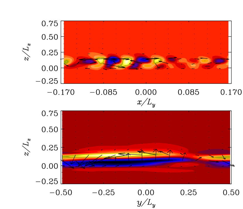
Figure 3: Top: Velocity components $U_{y}$ (in color), $U_{x}$ and $U_{z}$ (vectors) in the plane $y=0$. Bottom: $U_{x}$ (in color), $U_{y}$ and $U_{z}$ (vectors) in the plane $x=0$. Both during the linear evolution phase of the run B128a.

3.2 Linear stage.

At first we verify that the instability is indeed driven by magnetic buoyancy. As the coefficients in Eqs. (2)–(5) are constant, the initial state (7) depends only on $z$, and the boundary conditions in the $x$ and $y$ directions are periodic, all eigensolutions $\boldsymbol{\psi}\in\left\{\rho,\mbox{\boldmath{$u$}},\mbox{\boldmath{$b$}},s\right\}$ of the linearized problem must have the form

$$\boldsymbol{\psi}(\mbox{\boldmath{$x$}},t)=\,\hskip 0.85358pt\hat{\!\boldsymbol{\psi}}(z)\,\mathrm{e}^{\displaystyle\mathrm{i}\left[2\pi(mx/L_{\rm x}+ny/L_{\rm y})-\omega t\right]},$$ (16)

where $m$ and $n$ are integers and $\omega=\omega_{\rm R}+\mathrm{i}\omega_{\rm I}$. Corresponding dispersion relations $\omega(m,n)$ have been established by applying perturbations of the form (16) with a variational principle in the non-rotating case (Fan, 2001) and with the set of linearized anelastic MHD equations in magnetostrophic approximation at finite angular velocity (Schmitt, 1985). The former case allows both oscillatory and non-oscillatory unstable modes, although in Fan (2001) only non-oscillatory modes are reported. In the latter case, however, all unstable modes turn out to be oscillatory with the ratio $\omega_{\rm R}/\omega_{\rm I}$ decreasing with latitude. Note that the analytic results of Schmitt (1985) are limited in their predictive power by the fact that the variables are not subjected to our specific boundary conditions and that the analysis is performed locally.

For the runs in Table 2 we find that in the early exponential growth phase $m=8$ and $n=1$ throughout as seen in Fig. 3 which shows a typical velocity pattern at a time during the linear stage.

This is consistent with the findings of Fan (2001) where the fastest growing mode had always the smallest possible (non-vanishing) wavenumber in the direction of the field whereas the wavenumber perpendicular to the field was high. According to the terminology of Fan we may qualify our eigenmodes as undular as they change periodically in the direction of the magnetic background field. In our case, there seems to be some mixing with lower $m$ modes since the growing perturbations do not appear to be perfectly sinusoidal. While the growth rates presented in Table 2 could be easily identified from the averaged quantities shown in Fig. 2, it was difficult to access the oscillation frequencies. This is because they are small compared to the growth rates and saturation sets in too early to allow for the observation of a complete oscillation period. Nevertheless, some indications for temporal variations in the eigenmode geometries have been found.

Generally, we observe an increase of the growth rate with increasing magnetic Prandtl number, but a decrease with increasing Prandtl number. We find that the growth rate increases with the Roberts number as shown in Fig. 4. This means that increasing efficiency of heat conduction in comparison to magnetic diffusion destabilizes the sub-adiabatic stratification in the system in agreement with the destabilizing effect of thermal diffusion studied by Acheson (1979).

Figure 4: Dependence of growth rate $\omega_{\rm I}$ on the inverse Roberts number derived from the runs in Table 2. Solid line: best linear fit. Size of circles codes for the value of Re (length-based, see Tab. 2).

3.3 Dependence on initial magnetic field and rotation

Another piece of evidence for the magnetic character of the instability is its dependence on the initial magnetic field strength. From Fig. 5 we see a clear increase of the growth rate and saturation level with decreasing $\,\hskip 0.85358pt\widetilde{\!\beta}_{0}$, that is, increasing $\mbox{\rm Lu}_{0}$, while keeping the rotation rate fixed at $\mbox{\rm Ta}_{\rm M}=3.24\times 10^{10}$. Schmitt (2000) predicted a growth rate $\propto v_{A0}^{2}/\Omega$ for finite rotation, in the magnetostrophic approximation, inversely proportional to $\zeta=\,\hskip 0.85358pt\widetilde{\!\beta}_{0}\sqrt{Ta_{\rm M}}$.

Next we keep $\,\hskip 0.85358pt\widetilde{\!\beta}_{0}$ constant at 2.27 and decrease $\zeta$ gradually from $4.09\times 10^{5}$ to 0. Inspecting Fig. 5, we find that growth rate and saturation level of $\langle B_{x}^{2}+B_{z}^{2}\rangle$ increase monotonically and reach their maxima at $\zeta=0$ ($\Omega=0$) while the saturation time is decreasing. The impeding effect of rotation onto the instability at large $\Omega$ is plausible in view of the Taylor-Proudman theorem because the unstable eigenmodes do show pronounced $z$ gradients in $U$, see Fig. 3.

$\scriptstyle\boldsymbol{(\,\hskip 0.85358pt\widetilde{\!\beta}_{0},\>\>\,10^{-5}\zeta)}$

Figure 5: Dependence of the instability on initial magnetic field strength, expressed by $\,\hskip 0.85358pt\widetilde{\!\beta}_{0}$ and rotation, expressed by $\zeta=\,\hskip 0.85358pt\widetilde{\!\beta}_{0}{\mathrm{Ta}_{\mathrm{M}}}^{1/2}$. Upper panel: rms value of the generated magnetic field components $\langle B_{x}^{2}+B_{z}^{2}\rangle$. Lower panel: $\langle B_{y}^{2}\rangle$. Legend shows $(\,\hskip 0.85358pt\widetilde{\!\beta}_{0},10^{-5}\zeta)$. $\Pr=\mbox{\rm Pr}_{\rm M}=1$, colatitude $\theta=30^{\circ}$, resolution $64^{3}$ throughout. Note that the normalization time $t_{\rm A0}$ is not the same for all curves, but proportional to $\,\hskip 0.85358pt\widetilde{\!\beta}_{0}^{1/2}$.

3.4 Saturated stage.

At later time the instability reaches saturation, characterized by turbulent magnetic, velocity, density and temperature fields, that decay slowly thereafter. However, in most of the analysis below, this decay will be ignored and the turbulence approximately statistically stationary. The turbulence is necessarily both inhomogeneous and anisotropic and we shall further show that it is also helical. Under such conditions we expect the emergence of a mean electromotive force. Indeed magnetic fields perpendicular to the initial magnetic layer are produced having non-vanishing horizontal averages.

$\Pr=0.125$, $\mbox{\rm Pr}_{\rm M}=0.125$, $\mbox{\rm Re}=8.2$
  
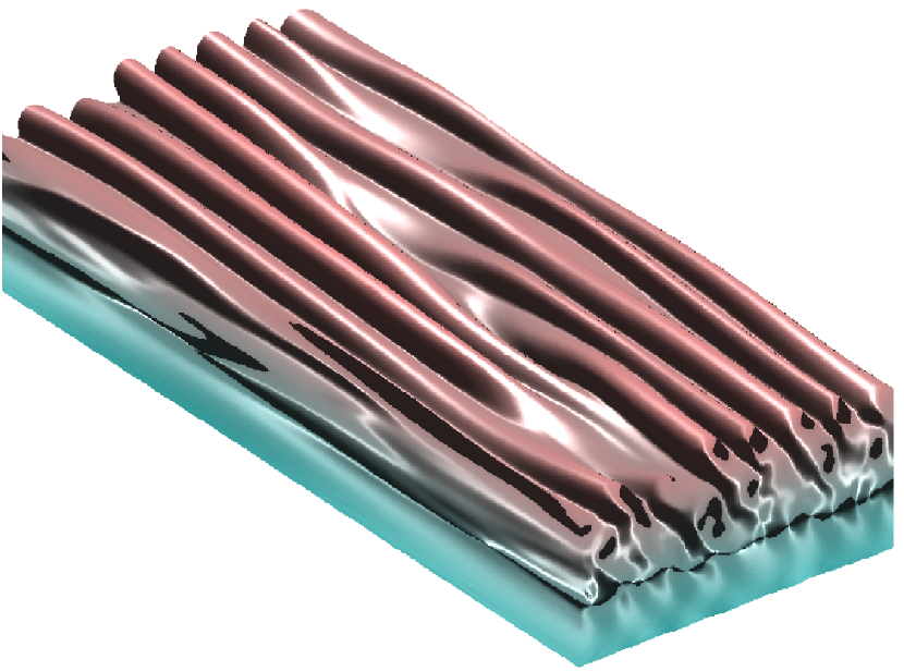
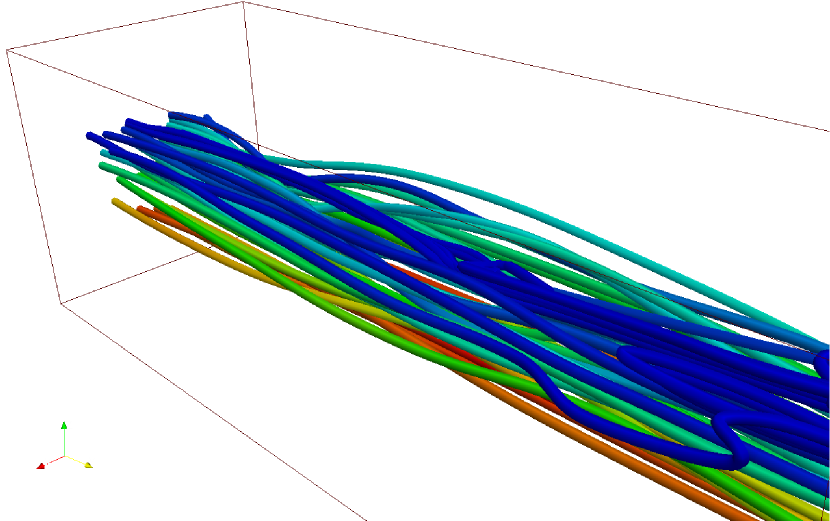
$\Pr=0.125$, $\mbox{\rm Pr}_{\rm M}=0.5$, $\mbox{\rm Re}=3.6$
  

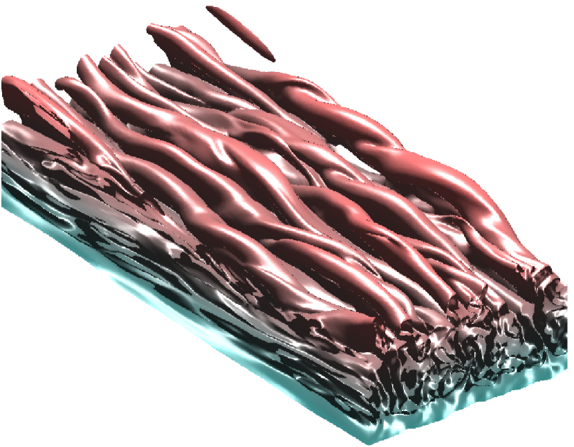
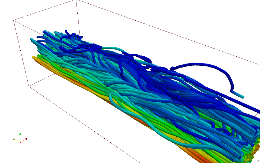
Figure 6: Left: volume rendering of the $B_{y}=0.1B_{0}$ isosurface. Right: field lines, colored according to the value of $B_{y}$ for runs B128f (top) and B128e (bottom) at $t=2t_{\rm A0}$ (saturated stage).

In order to give a better idea of the 3D geometry of the magnetic field we provide in Fig. 6 a volume rendering of $B_{y}$ at a time after $t^{\mathrm{sat}}$ for the runs B128e and B128f (see Table 2) which differ only in their magnetic Prandtl numbers. Notice how the magnetic layer breaks into flux tubes – similar to what is seen in Fig. 3 of Fan (2001) and also in Matthews et al. (1995). The difference between the two cases is most striking in the nature of corrugation in the surface shown. We attribute the difference to larger twist in the rising tubular structures in the run B128e compared to B128f which becomes clearly visible in the field line pictures also depicted in Fig. 6 (right).

$\delta\rho/\rho_{i}$

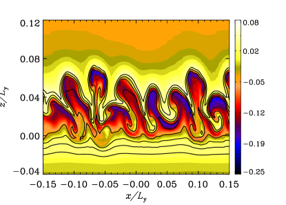
                                                                 $\delta T/T_{i}$

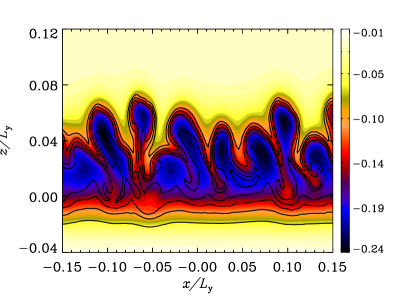
Figure 7: Relative density perturbation, $\delta\rho/\rho_{i}$ (top) and relative temperature perturbation $\delta T/T_{i}$ (bottom), with $\delta\rho=\rho-\rho_{i}$, $\delta T=T-T_{i}$ and $\rho_{i}(z)$, $T_{i}(z)$ taken from Eq. (7), in the plane $y=0$ at $t=t^{\rm sat}\sim 2t_{\rm A0}$ for the run B128h. Both plots overlaid with contours of $B_{y}$ (solid lines).

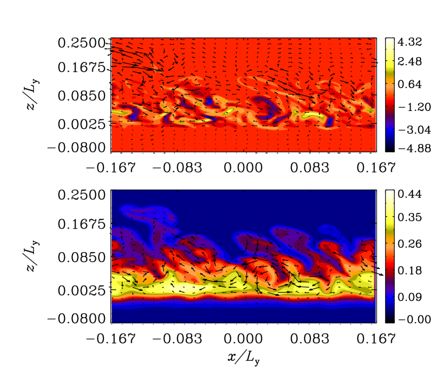
Figure 8: Scaled current helicity ${\boldsymbol{J}}\cdot{\boldsymbol{B}}/J_{\rm rms}B_{\rm rms}$ for run B128d (top) at $t=t^{\rm sat}\sim 2t_{\rm A0}$. Arrows show $v_{x}$ and $v_{z}$. $B_{y}/B_{y0}$ (bottom) for the same run. Arrows show $B_{x}$ and $B_{z}$. Both panels show the plane $y=0$.

Figure 7 demonstrates the breakup of the magnetic layer into tubular structures of concentrated magnetic field which are also regions of low density, hence rising. Notice also the high density regions just above and below these tubular structures. They show a significantly lower temperature than their surroundings (Fig. 7, bottom).

Considering the solar convection zone it is suggestive to ask to what extent the flux tubes are twisted, as their ability to rise over a large distance depends crucially on this property. For a quantitative measurement we utilize the dimensionless parameter $\varepsilon_{J}=\langle\mbox{\boldmath$J$}{}\cdot\mbox{\boldmath$B$}{}\rangle/J_{\mathrm{rms}}B_{\mathrm{rms}}$, the relative current helicity, essentially measuring the overall degree of alignment between $B$ and $J$. Here, angular brackets denote volume averages. A corresponding localized quantity is $\epsilon_{J}(z)=\overline{\mbox{\boldmath$J$}{}\cdot\mbox{\boldmath$B$}{}}/J_{\mathrm{rms}}B_{\mathrm{rms}}$. Figure 8 shows $\varepsilon_{J}$ (filled contours) as well as $B_{y}$ in the plane $y=0$ for run B128e. Notice that the contours are bend leftward because of the Coriolis force with $\mbox{\boldmath{$\Omega$}}\cdot\mbox{\boldmath{$\hat{z}$}}>0$. The contour plots of $B_{y}$ in this figure also show the formation of rising tubular structures from the magnetic layer.

In Fig. 9 we show the dependence of $\varepsilon_{J}$ on $\mathrm{Rb}$ and the profiles $\epsilon_{J}(z)$ for some selected runs. Although the total helicity reaches only values of a few percent, its localized counterpart is as strong as $30\%$ near to the initial location of the magnetic sheet. The clear dependence of $\varepsilon_{J}$ on $\mathrm{Rb}$ is in contrast to the only weak dependences on $\rm Pr_{\rm M}$ and $\rm Pr$ individually. This is an important result from this section. Our conjecture is that, at large $\mathrm{Rb}$, this magnetic buoyancy instability may play an important role in the formation of twisted flux tubes in the Sun, where $\mathrm{Rb}\gg 1$ is expected.

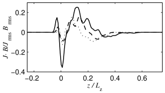
Figure 9: Top: Dependence of the total relative current helicity $\varepsilon_{J}$ on inverse Roberts number. Size of circles codes for value of $\mbox{\rm Re}_{\rm M}$. Bottom: Dependence of $\overline{\mbox{\boldmath{$J$}}\cdot\mbox{\boldmath{$B$}}}/J_{\rm rms}B_{\rm rms}$ on $z$ after saturation for runs B128e (solid, $\mathrm{Rb}^{-1}=0.25$), B128h (dashed, $\mathrm{Rb}^{-1}=0.5$), and B128c (dotted, $\mathrm{Rb}^{-1}=1$).

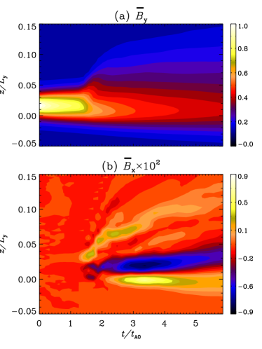
Figure 10: Time-depth diagram for $\overline{B}_{x,y}$ normalized on $B_{0}$ for run B128g in Table 2 ($z$ extent of the box clipped). Note the difference of two orders of magnitude between $\overline{B}_{y}$ and $\overline{B}_{x}$.

To demonstrate the emergence of a mean magnetic field we present in Fig. 10 time-depth plots of $\overline{B}_{y}$ and $\overline{B}_{x}$ for the run B128g (note that $\overline{B}_{z}=0$). There, $t\approx 1.6\,t_{\rm A0}$ marks the end of the exponential growth phase after which a strong growth of $\overline{B}_{x}$, obviously at the expense of $\overline{B}_{y}$, sets in. $\overline{B}_{x}$ reaches its maximum around $t\approx 3t_{\rm A0}$ and is then subject to the overall decay. Note the strong vertical concentration of $\overline{B}_{x}$, approximately antisymmetric about the midplane of the magnetic sheet.

3.5 Calculation of turbulent transport coefficients

The turbulence resulting from the buoyancy instability generates a mean magnetic field component $\overline{B}_{x}$ from an initial $\overline{B}_{y}$ which is also modified compared to its initial shape (see Fig. 10). It is then natural to employ the technique known as the quasi-kinematic test-field method to calculate transport coefficients like the $\alpha$ and $\eta$ tensors which describe this process. So far, test-fields have mostly been used in situations where a hydrodynamic background was already present in absence of the mean magnetic field (see, e.g. Brandenburg et al., 2008a, b, c). Here, in contrast, the (magnetohydrodynamic) turbulence results entirely from the instability of a pre-existing mean magnetic field, $B_{y0}(z)$. In other words, our simulations do not posses a kinematic stage in which the influence of $\overline{\mbox{\boldmath$B$}}{}$ would be negligible. One might worry that in such a situation the quasi-kinematic test-field method fails (Courvoisier et al., 2010). However, Eq. (13) continues to be valid and hence all conclusions drawn from it, because the decisive applicability criterion is whether or not there exists hydromagnetic turbulence in the absence of the mean magnetic field. This is not the case here, so the method should be applicable. The only peculiarity occurring is the fact that all components of $\alpha$ and $\eta$ vanish for $0\leq\overline{B}_{\mathrm{rms}}\leq\overline{B}_{\mathrm{threshold}}$, because fluctuating velocity and magnetic fields develop only after the instability has set in. Another aspect not considered in most previous test-field studies is the strong intrinsic inhomogeneity of the turbulence not only as a consequence of the strong $z$ dependence of $\overline{\mbox{\boldmath$B$}}{}$, but also due to the stratified density background. Thus the transport coefficients need to be determined as $z$ dependent quantities. We shall next demonstrate that the test-field method still works reasonably well in this regime. Note that to calculate the transport coefficients in addition to the usual MHD equations four additional evolution equations of the form (13) for four independent test-fields have to be solved. Hence the test-field runs are computationally almost thrice as expensive. We have thus reduced resolution to $64^{3}$ grid points for all these runs.

3.5.1 Reconstruction of the mean EMF

To validate the test-field method we first confirm that the quantity $\overline{\mbox{\boldmath${\cal E}$}}{}$, taken directly from the DNS, can be reproduced by employing the relation (11) between $\overline{\mbox{\boldmath${\cal E}$}}{}$ and $\overline{\mbox{\boldmath$B$}}{}$ with the tensors $\alpha$ and $\eta$ determined using the quasi-kinematic test-field method. In mathematical terms,

$$\overline{\cal E}{}_{i}^{\rm R}(z;\overline{\mbox{\boldmath$B$}}{})\!=\!\sum_{k}\!\big{[}\hat{\cal K}^{\mathrm{c}}_{ij}(z,k;\overline{\mbox{\boldmath$B$}}{})\,\hskip 0.85358pt\hat{\!B}^{\mathrm{c}}_{j}(k)+\hat{\cal K}^{\mathrm{s}}_{ij}(z,k;\overline{\mbox{\boldmath$B$}}{})\,\hskip 0.85358pt\hat{\!B}^{\mathrm{s}}_{j}(k)\big{]}$$ (17)

with

$$\begin{aligned} \hat{\cal K}_{ij}^{\mathrm{c}}&=\hat{\alpha}_{ij}(z,k^{\mathrm{c}};\overline{\mbox{\boldmath$B$}}{})\cos(k^{\mathrm{c}}\,\hskip 0.85358pt\widetilde{\!z})&&-\hat{\eta}_{il}(z,k^{\mathrm{c}};\overline{\mbox{\boldmath$B$}}{})\epsilon_{lj3}k^{\mathrm{c}}\sin(k^{\mathrm{c}}\,\hskip 0.85358pt\widetilde{\!z}),\\ \hat{\cal K}_{ij}^{\mathrm{s}}&=\hat{\alpha}_{ij}(z,k^{\mathrm{s}};\overline{\mbox{\boldmath$B$}}{})\sin(k^{\mathrm{s}}\,\hskip 0.85358pt\widetilde{\!z})&&+\hat{\eta}_{il}(z,k^{\mathrm{s}};\overline{\mbox{\boldmath$B$}}{})\epsilon_{lj3}k^{\mathrm{s}}\cos(k^{\mathrm{s}}\,\hskip 0.85358pt\widetilde{\!z}),\\ \end{aligned}$$

$$\begin{aligned} \,\hskip 0.85358pt\hat{\!B}^{\mathrm{c}}_{j}(k)&=\frac{2}{L_{z}}\int_{z}\overline{B}_{j}(z)\cos(k^{\mathrm{c}}\,\hskip 0.85358pt\widetilde{\!z})\,{\rm d}{}z,\\ \,\hskip 0.85358pt\hat{\!B}^{\mathrm{s}}_{j}(k)&=\frac{2}{L_{z}}\int_{z}\overline{B}_{j}(z)\sin(k^{\mathrm{s}}\,\hskip 0.85358pt\widetilde{\!z})\,{\rm d}{}z,\end{aligned}$$ (18)

$$\hskip 2.84526ptk^{\mathrm{c}}=\frac{(2k-1)\pi}{L_{z}},\quad k^{\mathrm{s}}=\frac{2k\pi}{L_{z}},\quad k=1,2,\ldots,$$

$$\quad\,\hskip 0.85358pt\widetilde{\!z}=z-z_{0}-\frac{L_{z}}{2},$$

where the superscript R indicates reconstruction. Here, the boundary condition for $B$ gives rise to the selection of discrete cosine and sine modes with wavenumbers $k^{\mathrm{c}}$ and $k^{\mathrm{s}}$, respectively. The additional argument $\overline{\mbox{\boldmath$B$}}{}$ is to indicate that the kernels $\boldsymbol{\hat{\cal K}^{\mathrm{c},\mathrm{s}}}$, as well as the tensors $\alpha$ and $\eta$, are valid just for that mean field $\overline{\mbox{\boldmath$B$}}{}$ which is present in the main run. As a consequence, the reconstruction of the mean EMF can be successful only when employing exactly this $\overline{\mbox{\boldmath$B$}}{}$ in (18). That is, the mean field representation of the turbulence by $\alpha$ and $\eta$ has, at this level, merely descriptive rather than predictive potential.

Let us denote $\overline{\mbox{\boldmath${\cal E}$}}{}^{\rm R}$ as the reconstructed EMF according to Eq. (17) truncated at $k^{\prime}\leq k_{\mathrm{max}}$, with $k^{c,s}=2k^{\prime}\pi/L_{z}$. Here $k^{\prime}$ can now take both integer and half-integer values where the integer (half-integer) values of $k^{\prime}$ correspond to the family of sine (cosine) modes in Eq. (18). An initial estimate of $k_{\mathrm{max}}$ required for a reasonable reconstruction of $\boldsymbol{\overline{\cal E}{}}$ was obtained from the power spectra of both $\overline{B}_{x}$ and $\overline{B}_{y}$. It turned out that $\overline{B}_{x}$ has significant spectral power up until $k^{\prime}=16$, whereas for $\overline{B}_{y}$ the power spectra has levelled off already at $k^{\prime}=8$. The components of the tensors $\alpha$ and $\eta$ also show rather different spectral behavior, both in the midplane of the magnetic layer and near the midplane of the box as seen in Fig. 11. From the figures it is evident that in most cases the spectra can be reasonably truncated at $k^{\prime}=8$ with the exceptions of $\alpha_{12}$ and $\alpha_{21}$. Note that the values for $k^{\prime}=0$ are not relevant here as, due to the boundary conditions, $\overline{\mbox{\boldmath$B$}}{}$ does not possess a $k^{\prime}=0$ contribution. The result of the assembly of $\overline{\mbox{\boldmath${\cal E}$}}{}^{\rm R}$ from (17) with (18), is presented in Fig. 12, middle column. From simple visual inspection we find it to be a faithful reproduction of $\overline{\mbox{\boldmath${\cal E}$}}{}$ from the DNS shown in the left column. Clearly, a naive application of the test-field procedure with harmonic test fields with only the lowest $k^{\prime}=0.5$ results in an inadequate description as shown in the right column.

   

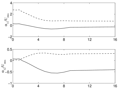
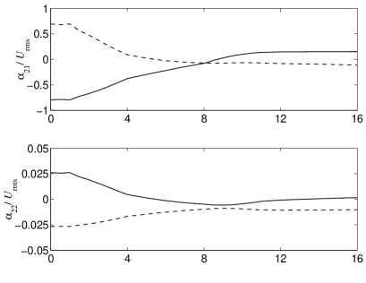
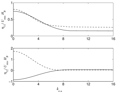
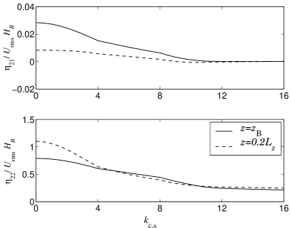
Figure 11: Dependence of $\alpha$ and $\eta$ on the test-field wavenumber $k^{\prime}$ in the midplane of the magnetic layer ($z=z_{B}$) and near the midplane of the box ($z=0.21L_{z}$) for run TF30+ of Table. 3. Integer and half-integer values of $k^{\prime}$ belong to sine and cosine modes in $\overline{\mbox{\boldmath$B$}}{}$, respectively. Note that $k^{\prime}=0$ refers to constant and linear test fields and that the coefficients for that value do not enter the $\overline{\mbox{\boldmath${\cal E}$}}{}$ - $\overline{\mbox{\boldmath$B$}}{}$ relation for the given setup.

$\overline{\cal E}{}_{x}$

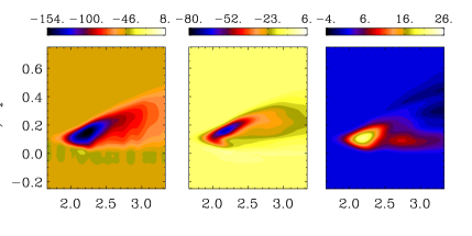
  $\overline{\cal E}{}_{y}$

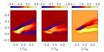
Figure 12: Reconstruction of the mean EMF for the run TF30+ using $\alpha$ and $\eta$ from the test-field method. Top: $\overline{\cal E}{}_{x}(z,t)$, bottom: $\overline{\cal E}{}_{y}(z,t)$, both scaled by $10^{-4}v_{\rm A0}B_{0}$. Left: directly from $\overline{{\boldsymbol{u}}\times{\boldsymbol{b}}}$. Middle: Reconstruction using all contributions $k^{\prime}=0.5,1,1.5,...16$ in (17). Right: Same as before, but using only the $k^{\prime}=0.5$ contribution.

We define two measures for the quality of the mean EMF reconstruction namely $\chi^{2}_{k^{\prime}}$ and the correlation coefficient $r_{k^{\prime}}$ defined as

$$\chi^{2}_{k^{\prime}}=\frac{\langle(\overline{\cal E}{}_{x,y}-\overline{\cal E}{}^{{\rm R}}_{x,y})^{2}\rangle_{z,t}}{\langle\overline{\cal E}{}_{x,y}^{2}\rangle_{z,t}},\hskip 4.2679ptr_{k^{\prime}}=\frac{\langle\overline{\cal E}{}_{x,y}\times\overline{\cal E}{}^{\rm R}_{x,y}\rangle_{z,t}}{\sqrt{\langle\overline{\cal E}{}_{x,y}^{2}\rangle_{z,t}\langle\overline{\cal E}{}^{\rm R2}_{x,y}\rangle_{z,t}}},$$ (19)

where the subscript “$z,t$” denotes that the averaging has been carried out over the vertical coordinate $z$ as well as over the temporal range $1.2t_{\rm A0}\leq t\leq 3.4t_{\rm A0}$. The relative error of the reconstruction, $\chi^{2}_{k^{\prime}}$, and the correlation coefficient, $r_{k^{\prime}}$, are plotted in Fig. 13 as a function of the truncation wavenumber $k_{\mathrm{max}}$. The $\chi^{2}_{k^{\prime}}$ reach a minimum value and level off around $k^{\prime}=8$ for both $\overline{\cal E}{}_{x}$ and $\overline{\cal E}{}_{y}$. This implies that including higher harmonic test fields beyond $k^{\prime}=7$ does not improve the reconstructed EMF. We speculate that the reason behind this discrepancy is that we have neglected memory effects (Hubbard & Brandenburg, 2009) in the turbulent transport coefficients. This can be particularly important in the present situation as we are obviously not in a statistically stationary regime. Similarly $r_{k^{\prime}}$ for $\overline{\cal E}{}^{\rm R}_{x}$ $(\overline{\cal E}{}^{\rm R}_{y})$ converges to a value of 0.98 (0.93) at $k^{\prime}=4$ $(8)$. It is important to note that even though the tensor components $\alpha_{12}$ and $\alpha_{21}$ do not converge with increasing $k^{\prime}$, the reconstructed EMFs do. Also calculating transport coefficients for $k^{\prime}\geq 8$ does not improve the reconstruction any further. This is probably because we do not sufficiently resolve wavenumber scales larger than $10$ in the domain with a grid resolution of only $64^{3}$.

Figure 13: Quality of the EMF reconstruction as a function of the truncation wavenumber $k_{\mathrm{max}}$: $\chi_{k^{\prime}}^{2}$ (left) and correlation $r_{k^{\prime}}$ (right) calculated for $\overline{\cal E}{}^{\rm R}_{x}$ (solid) and $\overline{\cal E}{}^{\rm R}_{y}$ (dashed) using Eq. (19).

3.5.2 Dependence of the transport tensors on inclination

From the point of view of the solar dynamo it is important to look at $\alpha$ and $\eta$ as functions of the rotational inclination $\theta$ or latitude $\lambda$, with a focus on symmetry properties with respect to $\lambda=0$, which is the solar equator. Moving from the northern hemisphere at $\lambda$ to the southern at $-\lambda$, that is changing $\theta$ to $\pi-\theta$, but keeping all other problem parameters constant, is equivalent to inverting the sign of $\Omega_{z}$. As the same can be accomplished by reflecting the corresponding rigid rotation about the plane $x=0$, we might construct the solution $(\rho,\mbox{\boldmath$U$}{},\mbox{\boldmath$B$}{},s)$ of (2)–(5) for $-\lambda$ simply by reflecting it properly about the same plane. Under this reflection polar vectors like velocity transform as,

$$\left\{U_{x},U_{y},U_{z}\right\}(x,y,z)\rightarrow\left\{-U_{x},U_{y},U_{z}\right\}(-x,y,z),$$ (20)

and axial vectors like the magnetic field as

$$\left\{B_{x},B_{y},B_{z}\right\}(x,y,z)\rightarrow\left\{B_{x},-B_{y},B_{z}\right\}(-x,y,z)$$ (21)

(Note that the gravitational acceleration is invariant under this reflection.) Hence, for the initial magnetic field, $B_{y0}(z)$, the transition to $-\lambda$ requires only a sign inversion. But, since the induction equation is linear in $B$, and Lorentz force as well as Ohmic dissipation are quadratic, inverting the sign of $B_{y0}(z)$ would just transform the solution $\{\rho,\mbox{\boldmath$U$}{},\mbox{\boldmath$B$}{},s\}$ to $\{\rho,\mbox{\boldmath$U$}{},-\mbox{\boldmath$B$}{},s\}$, that is, would leave the turbulence essentially unchanged and can be omitted. Moreover, as the transport coefficients, expressing correlation properties of the turbulent velocity $u$, are functions of $z$ only the reflection operation can hardly change their magnitudes. With respect to possible sign inversions we consider, that $\overline{\mbox{\boldmath${\cal E}$}}{}$ and $\overline{\mbox{\boldmath$J$}}{}$, being polar vectors, invert the sign of their $x$ components under reflection, but keep their $y$ components unchanged. The axial vector $\overline{\mbox{\boldmath$B$}}{}$ behaves just the opposite way. Thus, we have $\alpha_{ii}\rightarrow-\alpha_{ii}$ for $i=1,2$ (no summation) and $\alpha_{ij}\rightarrow\alpha_{ij}$ for $i\neq j$, whereas $\eta_{ii}\rightarrow\eta_{ii}$ for $i=1,2$ and $\eta_{ij}\rightarrow-\eta_{ij}$ for $i\neq j$ when moving from $\lambda$ to $-\lambda$. Consequently, it appears that the results for the southern hemisphere can be derived from those for the northern by simple operations. Strictly speaking however, this is only true when the initial condition for $U$ is also reflected upon the transition from $\lambda$ to $-\lambda$. From a naive point of view we might suppose that omitting this reflection can hardly be of any importance, because we use random initial condition. But this we have found not to be true. We note further that once the initial condition is reflected too the symmetry is restored.

According to the results of Schmitt (2000) we expect a decrease in the intensity of the instability with increasing inclination of the rotation axis. This can be explained by the buoyant nature of the turbulence, for which vertical motions are essential. At the poles, the effect of the Coriolis force on vertical motions is weakest, whereas they are strongly deflected at the equator. Figure 14 indeed confirms, that the growth rates decrease continuously when changing $\theta$ from $0^{\circ}$ towards $90^{\circ}$. In Fig. 15 we show the variation of the mean magnetic field and the corresponding mean EMF with latitude and $z$ at a time during the saturated stage. A pecularity in this figure is that $\overline{\cal E}{}_{y}$ and consequently $\overline{B}_{x}$ are non-zero at the equator where we would expect these quantities to vanish. This is an example of spontaneous symmetry breaking and can be explained by a mean field dynamo operating at the equator. This dynamo generates $\overline{B}_{x}$ whose sign is determined by the random initial conditions. A detailed discussion of this issue will be provided in a forthcoming paper. In the rest of the paper we anti-symmetrize $\overline{B}_{x}$ and $\overline{\cal E}{}_{y}$, while symmetrize $\overline{B}_{y}$ and $\overline{\cal E}{}_{x}$ about the equator (see Fig. 16). This is done by including the results from runs with two different initial conditions for velocity, one being the mirror reflection of the other according to Eq. (20). In particular at the equator ($\theta=90^{\circ}$), the two initial conditions give rise to a $\overline{B}_{x}$ with exactly the same magnitude but differing in sign. Thus averaging the $\overline{B}_{x}$ from the two runs gives a zero $\overline{B}_{x}$ at the equator. We perform the same operation for the turbulent transport coefficients calculated from the QKTF method. The transport coefficients calculated from only the $k^{\prime}=0.5$ test fields belonging to the family of cosine modes are presented in Fig. 17. It can be immediately seen from these plots that the instability becomes more effective with increasing (northern or southern) latitude. Corresponding runs performed with linear test-fields are compiled in Table 3. We observe that the turbulent transport coefficients increase in modulus when moving towards the poles, but are, with the only exception of $\alpha_{21}$, significantly reduced close to the equator. Obviously, the transport coefficients respond directly to the inhibition of the vertical motions by the Coriolis force when moving towards the equator.

Table 3: List of runs from set TF. $\Pr=4.0$, $\mbox{\rm Pr}_{\rm M}=4.0$, ${\mathrm{Ta}_{\mathrm{M}}}=3.24\times 10^{10}$, except for last three runs with ${\mathrm{Ta}_{\mathrm{M}}}=0$. $\,\hskip 0.85358pt\widetilde{\!\beta}_{0}=2.27$ except in last two runs, TF00l and TF00m, where $\,\hskip 0.85358pt\widetilde{\!\beta}_{0}$ is 3.22 and 1.03, respectively. Resolution $64^{3}$ throughout. Saturation is reached at $t^{\rm sat}$. Global extrema of the dominating $\overline{\cal E}{}_{y}$ with respect to $z$ and $t$ are given. $\mbox{\rm Re}\sim 4.8$ throughout. The arrows in the $\Omega$ column indicate the sign of $\Omega_{z}$.

Set	$\theta/^{\circ}$	$\Omega$	$t^{\rm sat}/t_{\mathrm{A0}}$	$10^{4}\times\overline{\cal E}{}_{y}/v_{\rm A0}B_{y0}$
				min	max
TF0$+$	0	$\uparrow$	2.42	$-1.82$	3.52
TF0$-$	0	$\downarrow$	2.42	$-4.41$	1.44
TF30$+$	30	$\uparrow$	2.58	$-1.71$	3.68
TF60$+$	60	$\uparrow$	2.87	$-1.33$	3.16
TF89$+$	89	$\uparrow$	3.00	$-1.21$	2.10
TF90$+$	90	$\uparrow$	3.50	$-1.35$	1.62
TF00	0	0	2.21	$-3.25$	3.12
TF00l	0	0	3.12	$-0.84$	1.38
TF00m	0	0	2.20	$-4.53$	8.43

Figure 14: Dependence of the instability on rotational inclination $\theta$ in terms of rms value of generated field components $\langle B_{x}^{2}+B_{z}^{2}\rangle$ for the runs TF$0+$, TF$30+$, TF$60+$ and TF$90+$ in Table. 3.

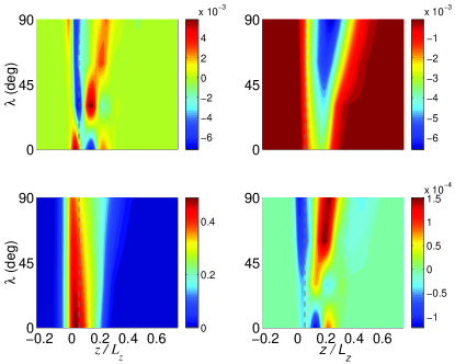
$\overline{B}_{x}/B_{0}$
                        $\overline{B}_{y}/B_{0}$
                                                                                         $\overline{\cal E}{}_{x}/v_{\rm A0}B_{0}$
                                                                                         $\overline{\cal E}{}_{y}/v_{\rm A0}B_{0}$

Figure 15: Latitudinal dependence of $\overline{B}_{x,y}(z)$, $\overline{\cal E}{}_{x,y}(z)$ averaged between $t=t^{\rm sat}$ and $t^{\rm sat}+t_{\rm A0}$. All problem parameters except $\theta$ held fixed at the values of run TF$0+$ in Table 3. Dashed line: initial position of the magnetic layer.

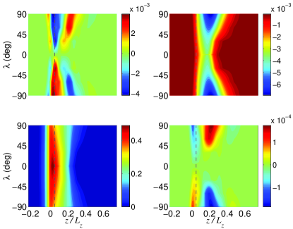
$\overline{B}_{x}/B_{0}$
                        $\overline{B}_{y}/B_{0}$
                                                                                         $\overline{\cal E}{}_{x}/v_{\rm A0}B_{0}$
                                                                                         $\overline{\cal E}{}_{y}/v_{\rm A0}B_{0}$

Figure 16: Same as Fig. 15 but now symmetrized about the equator.

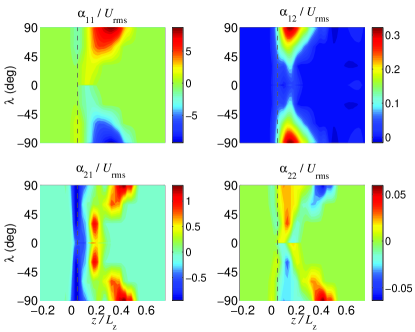
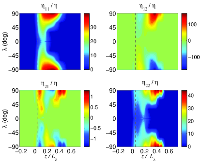
Figure 17: Dependence of $\alpha$ and $\eta$, averaged between $t=t^{\rm sat}$ and $t^{\rm sat}+t^{\rm A0}$, on latitude, $\lambda=90^{\circ}-\theta$, and $z$, calculated using test fields with $k^{\prime}=0.5$. All problem parameters except $\theta$ held fixed at the values of run TF$0+$ in Table 2. $\alpha$ scaled by $U_{\mathrm{rms}}$, $\eta$ scaled by the molecular diffusivity $\eta$. Dashed line: initial position of the magnetic layer.

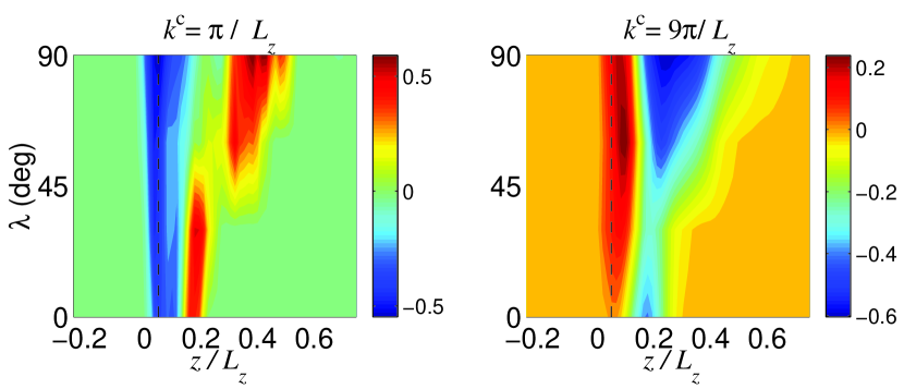
Figure 18: Pumping velocity $\gamma_{z}=(\alpha_{21}-\alpha_{12})/2$ scaled with $U_{\mathrm{rms}}$, as a function of latitude, $\lambda$ for $k^{\prime}=0.5$ (left panel) and $k^{\prime}=4.5$ (right panel).

The $\alpha$ tensor can be decomposed in symmetric and antisymmetric parts. The latter represents a turbulent pumping velocity $\boldsymbol{\gamma}$, and gives rise to the term $\boldsymbol{\gamma}\times\overline{\mbox{\boldmath$B$}}{}$ in the mean EMF. By virtue of the horizontal averaging of the magnetic field, $\overline{B}_{z}=0$. Hence, the only relevant component of pumping is $\gamma_{z}$ which is defined by $(\alpha_{21}-\alpha_{12})/2$. Analytical results indicate that in a wide range of situations, the turbulent pumping is directed away from the region of strong turbulence (“turbulent diamagnetism”, see Krause & Rädler, 1980). From Fig. 11, we see that the components $\alpha_{21}$ and $\alpha_{12}$ do not converge to zero with increasing $k^{\prime}$. In fact $\alpha_{12}$ changes sign at $k^{\prime}=2$ and $\alpha_{21}$ does so at $k^{\prime}=8$. Consequently ${\gamma_{z}}$ determined from harmonic test fields with $k^{\prime}=0.5$ and $k^{\prime}\geq 4$ should have opposite signs as confirmed by Fig. 18. Physically, this means that magnetic fields formed on the scale of $L_{z}$ will be pumped away from the initial magnetic layer while those on the scale of the magnetic layer, $H_{B}$ shall be pumped into the layer, the latter being contrary to the standard concept of “turbulent diamagnetism”. It is thus difficult to comment on the transport of the total $\overline{\mbox{\boldmath$B$}}{}$ by $\boldsymbol{\gamma}$. Only if the pumping were oriented away from the magnetic layer for all the wavenumbers of the dominating constituents in $\overline{\mbox{\boldmath$B$}}{}$ it would lead to a broadening of the initial layer i.e., a reduction of $\partial B_{y}/\partial z$ and would hence inhibit the instability. A similar dependence of turbulent pumping on wavenumber has been found by Käpylä, Korpi & Brandenburg (2009) in DNS of convection. With regard to to the saturation of the magnetic buoyancy instability, a strong turbulent magnetic diffusion given by $\eta_{22}$ (see Fig. 14) is likely to be more important. At the poles this quantity is as large as $40$ times the molecular value of $\eta$.

4 Conclusions

We have studied in detail the generation of the $\alpha$ effect due to the buoyancy instability of a toroidal magnetic layer in a stratified atmosphere by using direct numerical simulations. We find that both the magnetic energy and the current helicity in the system increase monotonically with the ratio of thermal conductivity to magnetic diffusivity, the Roberts number $\mathrm{Rb}$ (Fig. 4). This agrees with earlier analytical work of Gilman (1970) and Acheson (1979) as well as numerical work of Silvers et al. (2009) which find that efficient thermal diffusion or heat exchange can destabilize a stable stratification. The dependence of twist on $\mathrm{Rb}$ is an important result since the buoyancy instability would produce twisted flux tubes from a magnetic layer, if it existed in the overshoot layer of the Sun. Vasil & Brummel (2008) also reported the formation of twisted flux tubes from a horizontal magnetic layer produced, but in their case it is due to the action of shear on a weak vertical magnetic field. We further find that the growth rate of the buoyancy instability is reduced in presence of rotation compared to the case with $\Omega=0$.

We have run our simulations only until the time taken by the initial magnetic layer to break up due to the buoyancy instability. In absence of any other forcing such as a strong shear, the buoyancy instability cannot usually sustain itself past the break-up phase since the vertical gradient of the magnetic energy in the layer becomes comparable to the stratification due to magnetic diffusion. We may say that strong shear is not imperative to the production of tubular structures from the toroidal magnetic layer but will play a key role in keeping the layer from breaking up. It may also be possible that turbulent pumping arrests the decay of such a magnetic layer in the actual overshoot region. However, it is not yet clear if such a layer exists and is subject to the buoyancy instability in the real Sun.

We have ‘measured’ the turbulent transport coefficients using the technique of the quasi-kinematic test-field method. In order to prove that the $\alpha$ and $\eta$ tensors obtained from this method are reasonably accurate, we show the agreement between $\overline{\mbox{\boldmath${\cal E}$}}{}=\overline{\mbox{\boldmath{$u^{\prime}$}}\times\mbox{\boldmath{$b^{\prime}$}}}$ and the ansatz $\overline{\mbox{\boldmath${\cal E}$}}{}=\mbox{\boldmath$\alpha$}\overline{\mbox{\boldmath{$B$}}}-\mbox{\boldmath$\eta$}\overline{\mbox{\boldmath{$J$}}}$ using harmonic test fields with wavenumbers $0\leq k^{\prime}\leq 16$. Here we have illustrated a technique of judging the reliability of transport coefficients obtained from the test-field method. We find that, even in presence of magnetically driven turbulence, $\alpha$ and $\eta$ obtained from the quasi-kinematic test-field method provide a reasonably accurate description of the turbulent EMF. This is an important outcome of our study.

We find that $\overline{\cal E}{}_{x}$ determined using a harmonic test field with the lowest wavenumber that fits in vertical extent of the box already comprises a considerable part of the total EMF. Hence we can use QKTF to calculate the turbulent coefficients at finite $\Omega$ as a function of latitude using harmonic test fields with this wavenumber. The component $\alpha_{22}$ contributes to the generation of $\overline{B}_{x}$ from the strong initial field $\overline{B}_{y}$ in the layer. The off-diagonal components contribute to a vertical turbulent pumping velocity directed away from the region of turbulence surrounding the magnetic layer. The influence of this component systematically expands along $z$ with increasing latitude and somewhat agrees with the result in Brandenburg & Schmitt (1998). The agreement is not complete since the $\alpha_{22}(z,\theta)$ is inhomogeneous with respect to $z$ and can have sign changes along $\theta$, e.g., at $z/L_{z}=0.4$ in Fig. 17d. We find that all transport coefficients except $\alpha_{21}$ increase with latitude and are significantly reduced near the equator due to the suppressing effect of the Coriolis force on the instability.

For the first time the turbulent magnetic diffusivity given by the diagonal components of $\eta$ has been computed, as shown in Fig. 17. In particular, near the magnetic layer, the diagonal component $\eta_{22}$ is 25 times larger than the molecular value $\eta$. The buoyancy driven instability has the property that the $\alpha$ as measured by the growth rate of the instability increases with the magnitude of the magnetic field in the horizontal layer (compare solid and dashed lines Fig. 5). This property makes it an attractive candidate for solar dynamo models, unlike the $\alpha$ generated due to helical turbulence which gets quenched for strong magnetic fields. The increase of $\alpha$ and $\eta$ with $\overline{\mbox{\boldmath$B$}}{}$ is a remarkable result and supports similar suggestions by Brandenburg et al. (1998) that, if turbulent transport coefficients are caused by flows that are magnetically driven like here or, e.g., in Balbus-Hawley instabilities, then both $\alpha$ and $\eta$ may increase with the magnetic field strength. This trend is sometimes referred to as ‘anti-quenching’ and may be needed to support the observational relation between the ratio of dynamo cycle to rotation frequencies, $\omega_{\rm cyc}/\Omega$ and Rossby number inverse, $\rm{Ro}^{-1}$ for stellar data (Brandenburg et al., 1998; Saar & Brandenburg, 1999). Note finally that modelling the $\alpha$ as a function of space and the mean magnetic field to use in a mean field dynamo model is a very difficult proposition that needs to be postponed to future work.