Hardness and Approximation of
The Asynchronous Border Minimization Problem

We study a combinatorial problem arising from microarrays synthesis. The synthesis is done by a light-directed chemical process. The objective is to minimize unintended illumination that may contaminate the quality of experiments. Unintended illumination is measured by a notion called border length and the problem is called Border Minimization Problem (BMP). The objective of the BMP is to place a set of probe sequences in the array and find an embedding (deposition of nucleotides/residues to the array cells) such that the sum of border length is minimized. A variant of the problem, called P-BMP, is that the placement is given and the concern is simply to find the embedding.

Approximation algorithms have been proposed for the problem [22] but it is unknown whether the problem is NP-hard or not. In this paper, we give a thorough study of different variations of BMP by giving NP-hardness proofs and improved approximation algorithms. We show that P-BMP, 1D-BMP, and BMP are all NP-hard. Contrast with the result in [22] that 1D-P-BMP is polynomial time solvable, the interesting implications include (i) the array dimension (1D or 2D) differentiates the complexity of P-BMP; (ii) for 1D array, whether placement is given differentiates the complexity of BMP; (iii) BMP is NP-hard regardless of the dimension of the array. Another contribution of the paper is improving the approximation for BMP from $O(n^{1/2}\log^{2}n)$ to $O(n^{1/4}\log^{2}n)$, where $n$ is the total number of sequences.

1 Introduction

DNA and peptide microarrays [12, 7] are important research tools used in gene discovery, multi-virus discovery, disease and cancer diagnosis. Apart from measuring the amount of gene expression [28], microarray is an efficient tool for making a qualitative statement about the presence or absence of biological target sequences in a sample, for example peptide microarrays have been used for detecting tumor biomarkers [6, 24, 30]. A microarray is a plastic or glass slide (2D grid-like) consisting of thousands of short sequences called probes. Microarray design raises a number of challenging combinatorial problems, such as probe selection [13, 16, 23, 29], deposition sequence design [19, 25] and probe placement and synthesis [15, 3, 4, 5, 17, 18]. In this paper, we focus on the probe placement and synthesis problem.

The synthesis process [10] consists of two components: probe placement and probe embedding. Probe placement is to place each probe to a unique array cell and probe embedding is to determine a deposition sequence of masks to allow (and block) lights on the array cells (see Figure 1). The deposition sequence is a supersequence of all probes. Figure 2 shows the deposition sequence (ACGT)³ and various embeddings of the probe CGT, e.g., (a) shows the embedding ($-$)C($-$)⁴G($-$)⁴T, where “$-$” represents a space. The synthesis can be classified as synchronous and asynchronous synthesis. In the former, the $i$-th deposition character can only be deposited to the $i$-th position of the probes. In the later, there is no such restriction. Figure 1 shows asynchronous synthesis.

Due to diffraction, internal reflection and scattering, cells on the border between masked and unmasked regions are often subject to unintended illumination [10], and can compromise experimental results. As microarray chip is expensive to synthesize, unintended illumination should be minimized. The magnitude of unintended illumination can be measured by the border length of the masks used, which is the number of borders shared between masked and unmasked regions, e.g., in Figure 1, the border length of ${\mathcal{M}}_{1},{\mathcal{M}}_{3},{\mathcal{M}}_{4}$ is $2$ and ${\mathcal{M}}_{2}$ is $4$.

Synchronous synthesis. Hanannenhalli et al. [15] defined the Border Minimization Problem (BMP) for synchronous synthesis, in which the only concern is probe placement. Once the placement is fixed, the border length is proportional to the Hamming distance of neighboring probes. Hanannenhalli et al. [15] proposed an approximation algorithm based on travelling salesman path (TSP) in the complete graph representing the probes and their Hamming distance. Experiments have been carried out to show the effectiveness of the algorithm. Other algorithms [17, 18, 4] have been proposed to improve the experimental results. Recently, the problem has been proved to be NP-hard [20] and $O(\sqrt{n})$-approximable [21], where $n$ is the number of probes.

Asynchronous synthesis. In this paper, we focus on asynchronous synthesis, which was introduced by Kahng et al. [17]. The problem appears to be difficult as they studied a special case that the deposition sequence is given and the embeddings of all but one probes are known. A polynomial time dynamic programming algorithm was proposed to compute the optimal embedding of this single probe. This algorithm is used as the basis for several heuristics [3, 4, 5, 17, 18] that are shown experimentally to reduce unintended illumination. The dynamic programming mentioned above computes the optimal embedding of a single probe in time $O({\ell}|D|)$, where ${\ell}$ is the length of a probe and $D$ is the deposition sequence. The algorithm can be extended to an exponential time algorithm to find the optimal embedding of all $n$ probes in $O(2^{n}{\ell}^{n}|D|)$ time.

\psfrag{e1}{\footnotesize{$e_{1}=$}}\psfrag{e2}{\footnotesize{$e_{2}=$}}\psfrag{e3}{\footnotesize{$e_{3}=$}}\psfrag{e4}{\footnotesize{$e_{4}=$}}\psfrag{e5}{\footnotesize{$e_{5}=$}}\psfrag{M1}{\scriptsize{${\mathcal{M}}_{1}$}}\psfrag{M2}{\scriptsize{${\mathcal{M}}_{2}$}}\psfrag{M3}{\scriptsize{${\mathcal{M}}_{3}$}}\psfrag{M4}{\scriptsize{${\mathcal{M}}_{4}$}}\psfrag{M5}{\scriptsize{${\mathcal{M}}_{5}$}}\psfrag{A}{\tiny{A}}\psfrag{C}{\tiny{C}}\psfrag{G}{\tiny{G}}\psfrag{T}{\tiny{T}}\psfrag{AC}{\tiny{AC}}\psfrag{CA}{\tiny{CA}}\psfrag{CT}{\tiny{CT}}\psfrag{TA}{\tiny{TA}}\psfrag{unmasked region}{\scriptsize{unmasked region}}\psfrag{masked region}{\scriptsize{masked region}}\includegraphics[width=227.62204pt]{mask.eps}

Figure 1: Asynchronous synthesis of a $2\times 2$ microarray. The deposition sequence $D=$ CTAC corresponds to the sequence of four masks ${\mathcal{M}}_{1}$, ${\mathcal{M}}_{2}$, ${\mathcal{M}}_{3}$, and ${\mathcal{M}}_{4}$. The masked regions are shaded. The borders between the masked and unmasked regions are represented by bold lines. With respect to the deposition sequence $D$, the embedding of sequence AC is $--$AC, TA is $-$TA$-$, CT is CT$--$, CA is C$-$A$-$.

\psfrag{p}{\footnotesize{$p=$ CGT}}\psfrag{1}{\footnotesize{(a)}}\psfrag{2}{\footnotesize{(b)}}\psfrag{3}{\footnotesize{(c)}}\psfrag{4}{\footnotesize{(d)}}\psfrag{a}{\scriptsize{A}}\psfrag{c}{\scriptsize{C}}\psfrag{g}{\scriptsize{G}}\psfrag{t}{\scriptsize{T}}\psfrag{S}{{$D$}}\psfrag{E1}{{${\varepsilon}_{1}$}}\psfrag{E2}{{${\varepsilon}_{2}$}}\psfrag{E3}{{${\varepsilon}_{3}$}}\psfrag{E4}{{${\varepsilon}_{4}$}}\includegraphics[width=170.71652pt]{embedding.eps}

Figure 2: Different embeddings of probe $p=$ CGT into deposition sequence $D=(\mbox{ACGT})^{3}$.

To find both placement and embedding, Li et al. [22] proposed an $O(\sqrt{n}\log^{2}n)$-approximation algorithm. This is based on their $O(\log^{2}n)$-approximation for finding embeddings when placement is given. On a one-dimensional array, they showed that the approximation ratio could be improved to $3/2$. If in addition the placement is given, the problem can be solved optimally in polynomial time. It is however unknown whether the general problem is NP-hard or not. We note that the NP-hard proof in [20] cannot be applied to the asynchronous problem and it is not straightforward to show direct relation between the synchronous and asynchronous problems. This leaves several open questions in the asynchronous problem. Let us denote by P-BMP the problem with placement already given.

• So far only approximation algorithms for BMP have been proposed. An open question is whether BMP (or even 1D-BMP) is NP-hard.

• An exponential-time algorithm for P-BMP has been proposed while 1D-P-BMP can be solved optimally in polynomial time. Is P-BMP (on 2D array) NP-hard?

• Is it possible to improve existing approximation algorithms for BMP or P-BMP?

Setting	2D	1D
BMP	NP-hard∗	NP-hard∗
	$O(n^{1/4}\log^{2}n)$-approximate∗	$\frac{3}{2}$-approximate [22]
P-BMP	NP-hard∗	polynomial time solvable [22]
	$O(\log n)$-approximate∗

Table 1: Results on BMP and P-BMP. Results in this paper are marked with an asterisk.

Our contributions. We give a thorough study of different variations of the asynchronous border minimization problem. We answer the above questions affirmatively by giving several NP-hard proofs and better approximation algorithms. Our contributions are listed below (see Table 1 also):

• For 1D-BMP (placement not given), we give a reduction from the Hamiltonian Path problem [11] to 1D-BMP, implying the NP-hardness of 1D-BMP.
  This means that when the array is one dimension, whether placement is given differentiates the complexity of BMP (as 1D-P-BMP is polynomial time solvable [22]).

• We further show that 1D-BMP can be reduced to BMP and thus, BMP is NP-hard.
  This means that BMP is NP-hard regardless of the dimension of the array.

• For P-BMP, we show that the Shortest Common Supersequence problem [26] can be reduced to P-BMP, implying that P-BMP is NP-hard.
  This means that the dimension differentiates the complexity of P-BMP as we have seen in [22] that 1D-P-BMP is polynomial time solvable.

• We also improve the approximation ratio for P-BMP from $O(\log^{2}n)$ to $O(\log n)$ and BMP from $O(n^{1/2}\log^{2}n)$ to $O(n^{1/4}\log^{2}n)$.

Organization of the paper. In Section 2, we give some definitions and preliminaries. In Sections 3 and 4, we give the hardness results for P-BMP and BMP, respectively. In Section 5, we present and analyze an approximation algorithm for BMP. We conclude in Section 6.

2 Preliminaries

We are given a set of $n$ sequences ${\mathcal{S}}=\{s_{1},s_{2},\ldots,s_{n}\}$, a $\sqrt{n}\times\sqrt{n}$ array (for simplicity, we assume that $\sqrt{n}$ is an integer). For any sequence $s_{i}$, we denote the length of the sequence by $\ell_{i}$ and the $t$-th character of a sequence $s_{i}$ by $s_{i}[t]$. The probe sequences in ${\mathcal{S}}$ are to be placed on the $\sqrt{n}\times\sqrt{n}$ array. We denote a cell in the array as $v$. Two cells $v_{1}=(x_{1},y_{1})$ and $v_{2}=(x_{2},y_{2})$ are said to be neighbors if $|x_{1}-x_{2}|+|y_{1}-y_{2}|=1$. For each cell $v$, we denote the set of neighbors of $v$ by ${\mathcal{N}}(v)$.

Placement and embedding. A placement of the probe sequences is a bijective function ${\phi}$ that maps each probe sequence to a unique cell in the array. A deposition sequence $D$ is a sequence of characters and each character is deposited by a mask to some cells of the array. A mask ${\mathcal{M}}$ can be viewed as a 2D-array such that ${\mathcal{M}}(i,j)$ is either the character associated with ${\mathcal{M}}$ or a space “$-$”. The space means that the character is not deposited in this cell.

An embedding of a set of probes ${\mathcal{S}}$ into a deposition sequence $D$ is denoted by ${\varepsilon}=\{{\varepsilon}_{1},{\varepsilon}_{2},\ldots,{\varepsilon}_{n}\}$. For $1\leq i\leq n$, ${\varepsilon}_{i}$ is a length-$|D|$ sequence such that (1) ${\varepsilon}_{i}[t]$ is either $D[t]$ or a space $``-"$; and (2) removing all spaces from ${\varepsilon}_{i}$ gives $s_{i}$. There are two ways to define the border length between two probes $s_{i}$ and $s_{j}$. The Hamming distance between ${\varepsilon}_{i}$ and ${\varepsilon}_{j}$ measures $\textup{border}_{{\varepsilon}}(s_{i},s_{j})$. With this definition, $\textup{border}_{{\varepsilon}}(s_{i},s_{j})=\textup{border}_{{\varepsilon}}(s_{j},s_{i})$. We use this in Section 5. Sometimes, it is more convenient to define an asymmetric measurement, $\textup{border}^{\prime}_{{\varepsilon}}(s_{i},s_{j})$ is the number of $p$’s such that (i) ${\varepsilon}_{i}[p]\not=\text{`$-$'}$, and (ii) ${\varepsilon}_{i}[p]\not={\varepsilon}_{j}[p]$. Condition (ii) means that ${\varepsilon}_{j}[p]=\text{`$-$'}$. Note that $\textup{border}^{\prime}_{{\varepsilon}}(s_{i},s_{j})\not=\textup{border}^{\prime}_{{\varepsilon}}(s_{j},s_{i})$ while $\textup{border}_{{\varepsilon}}(s_{i},s_{j})=\textup{border}^{\prime}_{{\varepsilon}}(s_{i},s_{j})+\textup{border}^{\prime}_{{\varepsilon}}(s_{j},s_{i})$. We use this definition in Sections 3 and 4.

Border length. The border length of a placement ${\phi}$ and an embedding ${\varepsilon}$ is defined as the sum of borders over all pairs of probe sequences

$$\textup{BL}({\phi},{\varepsilon})=\frac{1}{2}\displaystyle\sum_{\scriptsize\begin{array}[]{c}s_{i},s_{j}:\\ {\phi}(s_{j})\in{\mathcal{N}}({\phi}(s_{i}))\end{array}}\textup{border}_{{\varepsilon}}(s_{i},s_{j})=\sum_{\scriptsize\begin{array}[]{c}s_{i},s_{j}:\\ {\phi}(s_{j})\in{\mathcal{N}}({\phi}(s_{i}))\end{array}}\textup{border}^{\prime}_{{\varepsilon}}(s_{i},s_{j})\,.$$ (1)

We can also define border length in terms of the border length of all the masks. For any mask ${\mathcal{M}}$ of deposition character $X$, the border length of ${\mathcal{M}}$, denoted by $\textup{BL}({\mathcal{M}})$, is defined as the number of neighboring cells $(i_{1},j_{1})$ and $(i_{2},j_{2})$ such that ${\mathcal{M}}(i_{1},j_{1})=X$ and ${\mathcal{M}}(i_{1},j_{1})\not={\mathcal{M}}(i_{2},j_{2})$. For a placement and embedding that corresponds to a sequence of masks ${\mathcal{M}}_{1}$, ${\mathcal{M}}_{2}$, $\cdots$, ${\mathcal{M}}_{d}$,

$$\textup{BL}({\phi},{\varepsilon})=\sum_{h=1}^{d}\textup{BL}({\mathcal{M}}_{h})$$ (2)

The objective is to find a placement ${\phi}$ and an embedding ${\varepsilon}$, so that $\textup{BL}({\phi},{\varepsilon})$ is minimized.

When the placement is given, we call the problem the P-BMP. We also consider the BMP when the array is one dimensional and we call the problem 1D-BMP.

WMSA and MRCT. As shown in [22], P-BMP can be reduced to the weighted multiple sequence alignment problem (WMSA), which in turn can be reduced to the minimum routing cost tree problem (MRCT). In the WMSA problem [2, 9, 14, 27], we are given $k$ sequences $S=\{S_{1},S_{2},\cdots,S_{k}\}$. An alignment is $S^{\prime}=\{S^{\prime}_{1},S^{\prime}_{2},\cdots,S^{\prime}_{k}\}$ such that all $S^{\prime}_{i}$ have the same length and $S^{\prime}_{i}$ is formed by inserting spaces into $S$. The problem is to minimize the weighted sum-of-pair score which is the weighted sum of pair-wise score of every pair of sequences in the alignment and the pair-wise score is the sum of distance of characters in each position of the two sequences. In the MRCT problem [1], we are given a graph with weighted edges. In a spanning tree, the routing cost between two vertices is the sum of weights of the edges on the unique path between the two vertices in the spanning tree. The MRCT problem is to find a spanning tree with minimum routing cost, which is defined as the sum of routing cost between every pair of two vertices.

The reduction results in [22] imply the following lemma.

Lemma 1 (​​[22]).

If there is a $c$-approximation for MRCT, there is a $c$-approximation for P-BMP.

It is stated in [22] that Bartal’s algorithm [1] finds a routing spanning tree by embedding a metric space into a distribution of trees with expected distortion $O(\log^{2}n)$. MRCT is $O(\log^{2}n)$-approximable [1]. Meanwhile, the ratio is improved to $O(\log n)$ by Fakcharoenphol, Rao and Talwar [8]. Together with Lemma 1, we have the following corollary.

Corollary 2.

There is an $O(\log n)$-approximation for the P-BMP.

Notice that we use the term embedding in two contexts, probe embedding refers to finding the deposition sequence while embedding a metric to trees is to obtain an approximation. This should be clear from the context and should not cause confusion.

3 P-BMP: Finding embedding when placement is given

We give a reduction from the Shortest Common Supersequence (SCS) problem to the P-BMP.

Shortest Common Supersequence problem. Given $n$ sequences of characters, a common supersequence is a sequence that contains all the $n$ sequences as subsequences. The Shortest Common Supersequence problem is to find a common supersequence with the minimum length.

The reduction is from the SCS problem over binary alphabet, which is known to be NP-hard [26]. Suppose that the binary alphabet is $\{0,1\}$. Consider an instance of the SCS problem with a set $S$ of $k$ binary strings $s_{1},\cdots,s_{k}$. Let $\ell_{i}$ be the length of $s_{i}$, $\ell=\max_{1\leq i\leq k}\ell_{i}$ be the length of the longest sequence in $S$, and $L=\sum_{1\leq i\leq k}\ell_{i}$. For any $1\leq p,q\leq\ell$, we define an instance for P-BMP, denoted by $I(p,q)$. As we show later, a shortest common supersequence can be found by computing the optimal solutions for a polynomial number of instances $I(p,q)$.

The input $I(p,q)$. We construct a $(2k+1)\times(2k+1)$ array. The probe sequences are over the alphabet $\{0,1,\$\}$, where $\$$ is a character different from 0 or 1.

• Except for row 2-4, each cell of row 1, 5, 6, 7, 8, $\cdots$ of the array contains the string “$”. We call these rows dummy-rows.

• All the cells of row 2 contain the same string “$0^{p}$”. We call this row all-0-row.

• All the cells of row 4 contain the same string “$1^{q}$”. We call this row all-1-row.

• Row 3 contains $s_{1}$, $s_{2}$, $\cdots$, $s_{k}$ in alternate cells, and the rest of the cells contain the string “$”, precisely, row 3 contains “$”, $s_{1}$, “$”, $s_{2}$, “$”, $\cdots$, “$”, $s_{k}$, “$”. We call this row seq-row.

Tables 2 and 3 show examples of $I(3,3)$ and $I(1,1)$, respectively.

Common supersequence and deposition sequence. Consider an instance $I(p,q)$, we need at least one mask for the dummy strings “$”, and the best is to use exactly one mask, say $M_{\$}$ for all these strings. For $M_{\$}$, row 1 (dummy-row) incurs a border length of $2k+1$ on the bottom boundary with all-0-row, and row 5 (dummy-row) incurs $2k+1$ on the top boundary with all-1-row. For seq-row, the border length on top boundary with all-0-row is $k+1$, on bottom boundary with all-1-row is also $k+1$, and within seq-row on left and right boundaries is $2k$. Therefore, the border length $\text{BL}(M_{\$})=4(2k+1)$. The total border length for $I(p,q)$ equals to $\text{BL}(M_{\$})$ plus that of the remaining deposition sequence, which in turn is related to a common supersequence of the sequences in $S$. Since the quantity $\text{BL}(M_{\$})$ is present in all the embeddings, we ignore this quantity when we discuss the border length for $I(p,q)$. The following lemma states a relationship between a common supersequence and an embedding of the probe sequences. Table 2 gives an example.

$	$	$	$	$	$	$
000	000	000	000	000	000	000
$	010	$	100	$	00	$
111	111	111	111	111	111	111
$	$	$	$	$	$	$
$	$	$	$	$	$	$
$	$	$	$	$	$	$

Table 2: $s_{1}=$ “010”, $s_{2}=$ “100”, $s_{3}=$“00”. The supersequence $D=$ “010011” is an optimal deposition sequence for $I(3,3)$. Ignoring the border of the mask for the dummy strings “$”, the optimal border length equals $2(p^{*}+q^{*})\times(2k+1)+2L=100$, where $p^{*}=q^{*}=k=3$ and $L=8$.

Lemma 3.

If $D$ is a common supersequence of the sequences in $S$ and the number of $0$’s and $1$’s in $D$ is $p^{*}$ and $q^{*}$, respectively, then $D$ is an optimal deposition sequence for $I(p^{*},q^{*})$ and the resulting optimal embedding has a border length of $2(p^{*}+q^{*})(2k+1)+2L$.

Proof.

First of all, it is easy to observe that $D$ is a deposition sequence for $I(p^{*},q^{*})$ because it is a common supersequence of sequences in $S$ and it has the same number of $0$’s and $1$’s in all-0-row and all-1-row of the array in $I(p^{*},q^{*})$, respectively. Notice that $p^{*}$ is at least the number of $0$’s in each of $s_{i}$ and similarly $q^{*}$ is at least the number of $1$’s. In the deposition sequence $D$, when $D[j]=0$, all-0-row incurs a border length of $2k+1$ on the top boundary with row 1 (dummy-row); all-0-row and seq-row together incur a border length of $2k+1$ on the bottom boundary; and a border length of $2x$ within seq-row, where $x$ is the number of cells on seq-row that 0 is deposited. A similar calculation can be done for the case when $D[j]=1$. As a whole, the total border length equals $2(p^{*}+q^{*})(2k+1)+2L$.

We further argue that this is the minimum border length for $I(p^{*},q^{*})$. In any deposition sequence, the number of 0’s is at least $p^{*}$ and the number of 1’s is at least $q^{*}$. Therefore, all-0-row and the cells with ‘0’ on seq-row together incur a border length at least $2p^{*}(2k+1)$, and similarly, all-1-row and the cells with ‘1’ on seq-row incur at least $2q^{*}(2k+1)$. The cell on seq-row with the sequence $s_{i}$ incurs $2\ell_{i}$ on the left and right boundaries, implying all these cells together incur $2L$. Therefore, no matter how we deposit characters to the cell, the total border length is at least $2(p^{*}+q^{*})(2k+1)+2L$. ∎

Lemma 3 implies that if $p+q$ is large enough, we have a formula for the optimal border length of the instance $I(p,q)$ in terms of $p$, $q$, and $L$. The following lemma considers the situation when $p+q$ is small. Table 3 gives an example.

$	$	$	$	$	$	$
0	0	0	0	0	0	0
$	010	$	100	$	00	$
1	1	1	1	1	1	1
$	$	$	$	$	$	$
$	$	$	$	$	$	$
$	$	$	$	$	$	$

Table 3: $s_{1}=$ “010”, $s_{2}=$ “100”, $s_{3}=$“00”. The shortest common supersequence is $D=$ “0100”. The optimal deposition for $I(1,1)$ is $D$. Ignoring the border of the mask for the dummy strings “$”, the optimal border length equals to $(2\times 7+2\times 7+2\times 3+2\times 2)+2\times 8=54$ (the first four terms refer to border length with top and bottom boundaries and the last term with left and right boundaries). On the other hand, $2(p^{*}+q^{*})\times(2k+1)+2L=44<54$, where $p^{*}=q^{*}=1$, $k=3$ and $L=8$.

Lemma 4.

If $D$ is a shortest common supersequence of the sequences in $S$ and the number of $0$’s and $1$’s in $D$ is $p^{*}$ and $q^{*}$, respectively, then for any $p_{1},q_{1}$ such that $p_{1}+q_{1}<p^{*}+q^{*}$, the optimal embedding for $I(p_{1},q_{1})$ has a border length greater than $2(p_{1}+q_{1})(2k+1)+2L$.

Proof.

Notice that any deposition sequence must be a common supersequence, and thus must have total length $\ell_{D}\geq p^{*}+q^{*}>p_{1}+q_{1}$. With this deposition sequence, the border length equals to $2\ell_{D}k+2(p_{1}+q_{1})(k+1)+2L>2(p_{1}+q_{1})k+2(p_{1}+q_{1})(k+1)+2L=2(p_{1}+q_{1})(2k+1)+2L$. The term $2(p_{1}+q_{1})k$ refers to the top and bottom border length for columns with $s_{i}$ in the seq-row while the term $2(p_{1}+q_{1})(k+1)$ is for columns with dummy string “$” in the seq-row. ∎

Using Lemmas 3 and 4, we can find the optimal solution for SCS from optimal solutions for P-BMP as follows. For all pairs of $1\leq p\leq\ell$ and $1\leq q\leq\ell$, we find the optimal solution to $I(p,q)$. If the border length of the optimal solution equals to $2(p+q)(2k+1)+2L$, there is a common supersequence of length $p+q$. Among all such pairs of $p$ and $q$, those with the minimum $p+q$ correspond to shortest common supersequences. Notice that there are a polynomial number of, precisely $\ell^{2}$, pairs of $p$ and $q$ to be checked. We then have the following theorem.

Theorem 5.

The P-BMP is NP-Hard.

4 BMP: Finding placement and embedding

We first give a reduction from the Hamiltonian Path problem to 1D-BMP (Section 4.1) and then a reduction from 1D-BMP to BMP (Section 4.2).

4.1 1D-BMP: BMP on a 1D array

Hamiltonian Path problem. In an undirected graph a Hamiltonian Path is a path which visits each vertex exactly once. Given an undirected graph, the problem is to decide if a Hamiltonian Path exists. It is known that the problem is NP-hard [11].

Constructing an instance of 1D-BMP from an instance of Hamiltonian Path problem. Consider an Hamiltonian Path instance in which the given graph is $G=(V,E)$, with $|V|=n$ and $|E|=m$. Suppose that the vertices are labelled as $V=\{1,2,\cdots,n\}$. For any edge between vertex $i$ and $j$ with $i<j$, we label the edge as $e_{i,j}$. We construct an instance $I$ of 1D-BMP of $n+2$ sequences to be placed on an array of size $1\times(n+2)$. The size of the alphabet is $m+2$. We now define the alphabet $\Sigma$ and the probe sequences $S$. See Figure 3 and Table 4 for an example.

\psfrag{v1}{\footnotesize{$v_{1}$}}\psfrag{v2}{\footnotesize{$v_{2}$}}\psfrag{v3}{\footnotesize{$v_{3}$}}\psfrag{v4}{\footnotesize{$v_{4}$}}\psfrag{v5}{\footnotesize{$v_{5}$}}\psfrag{v1e}{\footnotesize{$v_{1}:\quad e_{1,2}\,e_{1,5}$}}\psfrag{v2e}{\footnotesize{$v_{2}:\quad e_{1,2}\,e_{2,3}\,e_{2,4}$}}\psfrag{v3e}{\footnotesize{$v_{3}:\quad e_{2,3}\,e_{3,4}$}}\psfrag{v4e}{\footnotesize{$v_{4}:\quad e_{2,4}\,e_{3,4}\,e_{4,5}$}}\psfrag{v5e}{\footnotesize{$v_{5}:\quad e_{1,5}\,e_{4,5}$}}\includegraphics[height=71.13188pt]{graph.eps}

Figure 3: A given graph $G$ of the Hamiltonian Path problem and the corresponding vertex sequences.

$$$$$$	$e_{1,2}\,e_{1,5}$	$e_{1,2}\,e_{2,3}\,e_{2,4}$	$e_{2,3}\,e_{3,4}$	$e_{2,4}\,e_{3,4}\,e_{4,5}$	$e_{1,5}\,e_{4,5}$	######
$$$$$$	$e_{1,2}\,e_{1,5}$	$e_{1,2}\,e_{2,3}\,e_{2,4}$	$e_{2,3}\,e_{3,4}$	$e_{1,5}\,e_{4,5}$	$e_{2,4}\,e_{3,4}\,e_{4,5}$	######

Table 4: Referring to the graph $G$ in Figure 3, the placement on the top corresponds to vertex sequences in the order of a Hamiltonian path $v_{1},v_{2},v_{3},v_{4},v_{5}$, while the bottom one shows the order $v_{1},v_{2},v_{3},v_{5},v_{4}$, which is not a Hamiltonian path. For the placement on the top, we can deposit the edge characters as $e_{1,2},e_{2,3},e_{2,4},e_{3,4},e_{1,5},e_{4,5}$ and it can be seen that there is sharing for four edges in the Hamiltonian path $e_{1,2},e_{2,3},e_{3,4},e_{4,5}$. For the placement on the bottom, we can deposit using the same sequence, but there is sharing only for three edges, namely, $e_{1,2},e_{2,3},e_{4,5}$.

1. Alphabet: $\Sigma=\{e_{i,j}\mid e_{i,j}\in E\}\cup\{\$,\#\}$. We define an order on these characters such that $e_{i_{1},j_{1}}<e_{i_{2},j_{2}}$ if (i) $i_{1}<i_{2}$ or (ii) $i_{1}=i_{2}$ and $j_{1}<j_{2}$.

2. Probe sequences are divided into two types: vertex sequences and dummy sequences.

   • Vertex sequences: For vertex $i$ in $V$, we construct a vertex sequence $v_{i}$ such that $v_{i}$ is a string of the edge characters corresponding to all edges incident with it. The order of the edge characters in the string follows the same order defined in (1).

   • Dummy sequences: Furthermore, we add two dummy sequences $w_{\$}$ and $w_{\#}$ of length $n+1$ each, such that $w_{\$}=\$^{n+1}$, and $w_{\#}=\#^{n+1}$.

Notice that the length of each vertex sequence $v_{i}$ is at most $n-1$. Furthermore, for each vertex sequence, the order of the edge characters follows the order defined in (1). This implies that there exists a permutation of the edge characters such that it is a common supersequence of all vertex sequences and this forms a valid deposition sequence for all the vertex sequences.

The two dummy sequences $w_{\$}$ and $w_{\#}$ are to ensure that in an optimal placement they will be placed in the leftmost and the rightmost cells in the 1D array, otherwise, the border length would be too large. In other words, all the other vertex sequences $v_{i}$ will be placed in cells such that both left and right boundaries count.

We now claim that the graph $G$ has a Hamiltonian Path if and only if the optimal border length of the 1D-BMP instance $I$ is $2(n+1)+(4m-2(n-1))$. The first term $2(n+1)$ is for the two dummy sequences $w_{\$}$ and $w_{\#}$ and $4m-2(n-1)$ is for the vertex sequences $v_{i}$.

Suppose that there is an Hamiltonian Path in $G$. Without loss of generality, we assume that the Hamiltonian path is $v_{1},v_{2},\cdots,v_{n}$. We place the vertex sequences in this order in the cells of the array, with the leftmost and rightmost cells containing $w_{\$}$ and $w_{\#}$, respectively.

Consider any permutation of the edge characters such that it is a common supersequence of all vertex sequences. Suppose we use this sequence as the deposition sequence. Note that each edge character appears in exactly two vertex sequences. If there is no sharing between neighboring sequences, each edge character incurs border length of $2$ for each of the two vertex sequences, and the total border length would be $4m$. Since we place the vertex sequences according to the order in an Hamiltonian path, every edge character in this path is shared by two neighboring vertex sequences, thus, saving a border length of $2$. In total, we have $n-1$ edges $e_{i,i+1}$ in the Hamiltonian path, for $1\leq i\leq n-1$. Therefore, we can save $2(n-1)$, implying that the border length of the masks associated with edge characters is $4m-2(n-1)$. Together with the masks for the dummy characters, the total border length is $2(n+1)+4m-2(n-1)$.

Suppose that there is an embedding for $I$ with border length $2(n+1)+(4m-2(n-1))$. For the dummy sequences, they have to be placed at the leftmost and rightmost cells, otherwise, the border length incurred will be greater than $2(n+1)$. Each edge character only appears in two vertex sequences. So to have sharing for this character, we can only have these two sequences being neighbors in the graph $G$. So in order to save $2(n-1)$, we need each vertex sequence to share one character with its neighbor in the array, so the way the sequence in the array should lead to an Hamiltonian path.

With the above discussion, we conclude the following theorem.

Theorem 6.

The 1D-BMP is NP-Hard.

4.2 BMP on 2D array

In this section, we reduce the BMP on an $1\times n$ array to BMP on an $n\times n$ array. This implies that BMP is NP-hard. Consider an instance $I_{1}$ for 1D-BMP where there are $n$ sequences $s_{1},s_{2},\cdots,s_{n}$ over an alphabet $\Sigma$, and the length of $s_{i}$ is $\ell_{i}$. Let $\ell=\max_{1\leq i\leq n}\ell_{i}$. We construct an instance $I_{2}$ for BMP which contains two types of sequences, namely, the given sequence and the dummy sequence. The alphabet used is a superset of $\Sigma$, precisely, $\Sigma^{\prime}=\Sigma\cup\{x_{1},x_{2},\cdots,x_{n}\}\cup\{\$\}$. The instance $I_{2}$ is constructed as follows. Let $k>\ell$ be a large integer to be determined later.

• Dummy sequences: we create $n^{2}-n$ dummy sequences each containing one character $\$$.

• Given sequences: for each $s_{i}$, we create a length $k$ sequence $x_{i}^{k-\ell_{i}}\cdot s_{i}$.

We claim that the best way to place these $n^{2}$ sequences is to put the given sequences on the top row. In that case, the optimal solution for $I_{1}$ would give an optimal solution for $I_{2}$ and vice versa.

We now prove the claim. For each cell in the array, there are four boundaries, top, bottom, left, and right. A sequence placed in a certain cell contributes to the overall border length an amount of four times its length minus the sharing of characters with its four neighbors. Consider a sequence $s$, let us denote by $\textup{share}(s,s^{\prime})$ the number of characters that can be shared between two sequences $s$ and $s^{\prime}$. Let us also denote by $gs$, $ds$, and $b$ be a given instance, a dummy sequence, and the outmost boundary of the array. Then we have the following relationships.

$$\textup{share}(gs,gs)\leq\ell, \quad\textup{share}(gs,ds)=0, \quad\textup{share}(gs,b)=k,$$

$$\textup{share}(ds,ds)=1, \textup{share}(ds,b)=1$$

If we arrange all the sequences such that the given sequences are placed on the top row, we would have a sharing of $(n+2)\times\textup{share}(gs,b)=(n+2)k$. If any of these given sequences are not placed on the top row, we lose a sharing of at least $k$. No matter how the sequences are placed, the maximum sharing apart from those with the outmost boundaries of the array is at most $4n^{2}\ell$. If we set $k$ to be large enough, e.g., $k=4n^{2}\ell+1$, then any possible internal sharing (not with outmost boundaries) is not sufficient to compensate the loss of $k$. We have proved the claim that all the given sequences should be placed on the top row of the array and the following theorem follows from Theorem 6.

Theorem 7.

The (two-dimensional) BMP is NP-hard.

5 An $O(n^{\frac{1}{4}}\log^{2}{n})$ approximation algorithm for the BMP

In this section we present an $O(n^{\frac{1}{4}}\log^{2}{n})$ approximation algorithm for the BMP problem. This improves on the previous $O(\sqrt{n}\log^{2}{n})$ approximation. We use the approximation algorithm for the P-BMP (Corollary 2 in Section 2) as a blackbox.

First, we discuss the connection between the border length and the longest common subsequence. We denote the longest common subsequence between two probes $s_{i}$ and $s_{j}$, of lengths $\ell_{i}$ and $\ell_{j}$, by $LCS(s_{i},s_{j})$. The corresponding length is denoted by $|LCS(s_{i},s_{j})|$. For any probe embedding $\epsilon$, the maximum number of common deposition nucleotides between $s_{i}$ and $s_{j}$ is $|LCS(s_{i},s_{j})|$, in other words, $border_{\epsilon}(s_{i},s_{j})\geq\ell_{i}+\ell_{j}-2|LCS(s_{i},s_{j})|$. We define $d(s_{i},s_{j})=\ell_{i}+\ell_{j}-2|LCS(s_{i},s_{j})|$. We also observe that this distance measure is a metric on the set of input strings.

Therefore, if we can place the probes into the array such that the sum of the distances between any adjacent cells is within a factor $c$ of the optimum (we refer to this problem as the placement problem), then we can apply the $O(\log{n})$ approximation algorithm for the P-BMP and obtain an $O(c\log{n})$ approximation for the BMP. Formally, we want to find a permutation $\pi:\{1,\dots,n\}\to\{1,\dots,n\}$ such that the following quantity is minimized:

$$S(\pi)= \sum_{i=1}^{n-1}d(\pi(i),\pi(i+1))-\sum_{i=1}^{\sqrt{n-1}}d(\pi(i\sqrt{n}),\pi(i\sqrt{n}+1))$$

$$+\sum_{i=1}^{\sqrt{n}}\sum_{j=1}^{\sqrt{n-1}}d(\pi(i+(j-1)\sqrt{n}),\pi(i+j\sqrt{n}))$$

To see why the sum is defined in this way, imagine that the probes $\pi(1),\dots,\pi(\sqrt{n})$ are placed on the first row of the array in this order, $\pi(\sqrt{n}+1),\dots,\pi(2\sqrt{n})$ on the second row and so on.

The next proposition follows, given the previous observations.

Proposition 8.

A $c$-approximation algorithm for the placement problem implies an $O(c\log{n})$ approximation algorithm for the BMP.

Since it is difficult to find in polynomial time a permutation which optimizes the value $S$ on this general metric, we first embed the metric into a tree (in fact, into a distribution of trees) with $O(\log{n})$ distortion using the algorithm of Fakcharoenphol, Rao and Talwar [8] (the same algorithm used in the MRCT, and implicitly P-BMP, approximation). This idea, together with Proposition 8, gives us the following statement.

Proposition 9.

If we can approximate the placement problem on a tree (i.e., probes are associated to vertices in a tree and the distance between two probes is the length of the unique path between them) within a factor of $c$, then we have an $O(c\log^{2}{n})$ approximation to the BMP.

Our approximation algorithm for the placement problem on trees is very simple: we consider the ordering of the vertices given by an Euler tour of the tree. We then prove that this is an $O(n^{\frac{1}{4}})$ approximation algorithm for the placement problem on trees. Then, by Proposition 9 we are guaranteed to have an $O(n^{\frac{1}{4}}\log^{2}{n})$ approximation algorithm for the BMP problem.

The algorithm for the BMP problem is described formally in Algorithm 1.

Algorithm 1 The $O(n^{\frac{1}{4}}\log^{2}{n})$ approximation algorithm for the BMP

1:  Input: The strings $s_{1},s_{2},\dots,s_{n}$.

2:  Define $d(s_{i},s_{j})=\ell_{i}+\ell_{j}-2|LCS(s_{i},s_{j})|$

3:  Embed the metric given by this distance and the set of input points into a tree $T$ using the algorithm from [8].

4:  Let $\pi:\{1,2,\dots,n\}\to\{1,2,\dots,n\}$ be an Euler tour of the tree $T$.

5:  Place the probes in the array according to $\pi$: the probes $\pi(1),\dots,\pi(\sqrt{n})$ are placed on the first row of the array in this order, $\pi(\sqrt{n}+1),\dots,\pi(2\sqrt{n})$ on the second row and so on. (See Figure 4).

6:  Apply the P-BMP approximation algorithm.

7:  Output: The placement of the probes on the array based on the Euler tour and the embedding of the probes given by the P-BMP approximation algorithm.

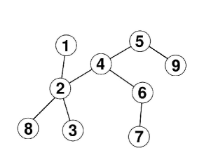
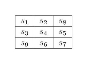
Figure 4: (a) Suppose the embedding in [8] returns such a tree for $9$ probes. (b) The placement of these probes on the array according to an Euler tour of the tree.

Before analyzing the algorithm, let us introduce a few notations. We denote by $T$ the tree obtained after the tree embedding. Notice that the cost of a solution is given by summing each edge of $T$ several times. We say that an edge $(x,y)\in T$ is crossed $r$ times in a solution $\pi$ if it is used $r$ times in the solution, i.e., it belongs to exactly $r$ of the $2\sqrt{n}(\sqrt{n}-1)$ paths of the solution.

Now, we want to find a lower bound for the optimal solution. We do so, by showing that in any solution, each edge of the tree has to be crossed at least a certain number of times. This is stated formally in the following lemma. Let $(x,y)\in T$ and denote by $A$ and $B$ the two connected components resulted from removing $(x,y)$.

Lemma 10.

In any permutation $\pi$ the edge $(x,y)$ is crossed at least $\sqrt{\min(|A|,|B|)}$ times.

Proof.

If we consider the probes placed on a grid graph (i.e., an $\sqrt{n}\times\sqrt{n}$ array), then the two sets of probes $A$ and $B$ determine a cut in the graph. We argue that the size of the cut is exactly the number of times the edge $(x,y)$ is crossed: for each edge $(\pi(i),\pi(j))$ in the cut, we have to add to the solution the corresponding path $\pi(i)\to\pi(j)$. But the path $\pi(i)\to\pi(j)$ has to cross the edge $(x,y)$, since $\pi(i)\in A$ and $\pi(j)\in B$. The minimum cut determined by two sets of size $|A|$ and $|B|$ has size $\sqrt{\min(|A|,|B|)}$ and therefore the lemma follows. ∎

We give an upper bound by considering the ordering of vertices given by an Euler tour of the tree.

Lemma 11.

In an Euler tour ordering, $(x,y)$ is crossed at most $O(\min(\sqrt{n},|A|,|B|))$ times.

Proof.

Due to the Euler tour, each edge can be crossed by edges from the paths $\pi(i)\to\pi(i+1)$ at most twice. Then we have to count how many edges from the paths $\pi(i)\to\pi(i+\sqrt{n})$ cross the edge $(x,y)$. We argue that $(x,y)$ cannot be crossed more than $4\min(|A|,|B|)$ times. Suppose $A$ is the set with the smaller cardinality. In the worst case for each element in $A$ all its four neighbors are in $B$ and, therefore $(x,y)$ is crossed $4\cdot\min(|A|,|B|)$ (this is actually too pessimistic but this suffices for our analysis since we are not interested in the precise constants).

We also argue that $(x,y)$ cannot be crossed more than $O(\sqrt{n})$ times. Since we follow an Euler tour, for an element $\pi(i)$, we have two cases: either $\pi(i+\sqrt{n})\in A$, or $\pi(i+\sqrt{n})\notin A$ and $\pi(j+\sqrt{n})\notin A,\forall j>i$. Therefore, for only $\sqrt{n}$ elements $\pi(i)$ of $A$, $\pi(i+\sqrt{n})$ is in $B$. The lemma then follows. ∎

Theorem 12.

The placement of the probes in the $\sqrt{n}\times\sqrt{n}$ array in the order given by the Euler tour gives an $O(n^{\frac{1}{4}}\log^{2}{n})$ approximation to the BMP problem.

Proof.

Consider an edge $(x,y)\in T$.

If $\min(|A|,|B|)\leq\sqrt{n}$, then $\min(\sqrt{n},|A|,|B|)/\sqrt{\min(|A|,|B|)}=\sqrt{\min(|A|,|B|)}\leq n^{\frac{1}{4}}$.

If $\min(|A|,|B|)>\sqrt{n}$, then $\min(\sqrt{n},|A|,|B|)/\sqrt{\min(|A|,|B|)}<\sqrt{n}/n^{\frac{1}{4}}=n^{\frac{1}{4}}$.

We then apply Proposition 9 and Lemmas 10 and 11 and the theorem follows. ∎

6 Concluding remarks

In this paper we give a thorough study of different variations of the Border Minimization Problem. We prove NP-hardness results and improved approximation algorithm. For P-BMP in which the position of the probes is given and the goal is to find the embedding, we show the hardness via a reduction from the Shortest Common Supersequence problem. For 1D-BMP (position not given) in which the array is an 1D array, we give an NP-hardness reduction from the Hamiltonian Path problem. We further show that 1D-BMP can be reduced to BMP and thus, BMP is NP-hard. We also give a better approximation algorithm for BMP.

Contrasting with the previous result in [22] that 1D-P-BMP is polynomial time solvable, our hardness results show that (i) the dimension differentiates the complexity of P-BMP; (ii) for 1D array, whether placement is given differentiates the complexity of BMP; (iii) BMP is NP-hard regardless of the dimension of the array.

In the reduction from Hamiltonian Path problem to 1D-BMP, the size of the alphabet is polynomial in terms of the number of sequences. An interesting question is whether 1D-BMP stays NP-hard even for constant of characters in the alphabet. Another natural open question is to further improve approximation algorithms for the problem and/or to derive inapproximability results.

References

- [1] Y. Bartal. Probabilistic approximations of metric spaces and its algorithmic applications. In FOCS, pages 184–193, 1996.
- [2] P. Bonizzoni and G. D. Vedova. The complexity of multiple sequence alignment with SP-score that is a metric. Theoretical Computer Science, 259(1–2):63–79, 2001.
- [3] S. A. Carvalho Jr. and S. Rahmann. Improving the layout of oligonucleotide. microarrays: Pivot partitioning. In Proc. 6th WABI, pages 321–332, 2006.
- [4] S. A. Carvalho Jr. and S. Rahmann. Microarray layout as quadratic assignment problem. In Proc. GCB, pages 11–20, 2006.
- [5] S. A. Carvalho Jr. and S. Rahmann. Improving the design of genechip arrays by combining placement and embedding. In Proc. 6th CSB, pages 54–63, 2007.
- [6] M. Chatterjee, S. Mohapatra, A. Ionan, G. Bawa, R. Ali-Fehmi, X. Wang, J. Nowak, B. Ye, F. A. Nahhas, K. Lu, S. S. Witkin, D. Fishman, A. Munkarah, R. Morris, N. K. Levin, N. N. Shirley, G. Tromp, J. Abrams, S. Draghici1, and M. A. Tainsky1. Diagnostic markers of ovarian cancer by high-throughput antigen cloning and detection on arrays. Cancer Research, 66(2):1181–1190, 2006.
- [7] M. Cretich and M. Chiari. Peptide Microarrays Methods and Protocols, volume 570 of Methods in Molecular Biology. Human Press, 2009.
- [8] J. Fakcharoenphol, S. Rao, and K. Talwar. A tight bound on approximating arbitrary metrics by tree metrics. In STOC, pages 448–455, 2003.
- [9] D. F. Feng and R. F. Doolittle. Approximation algorithms for multiple sequence alignment. Theoretical Computer Science, 182(1):233–244, 1987.
- [10] S. Fodor, J. L. Read, M. C. Pirrung, L. Stryer, A. T. Lu, and D. Solas. Light-directed, spatially addressable parallel chemical synthesis. Science, 251(4995):767–773, 1991.
- [11] M. R. Garey and D. S. Johnson. Computers and Intractability; A Guide to the Theory of NP-Completeness. Freeman, 1990.
- [12] D. Gerhold, T. Rushmore, and C. T. Caskey. DNA chips: promising toys have become powerful tools. Trends in Biochemical Sciences, 24(5):168–173, 1999.
- [13] L. Gąsieniec, C. Li, P. Sant, and P. Wong. Randomized probe selection algorithm for microarray design. Journal of Theoretical Biology, 248(3):512–521, 2007.
- [14] D. Gusfield. Efficient methods for multiple sequence alignment with guaranteed error bounds. Bulletin of Mathematical Biology, 55(1):141–154, 1993.
- [15] S. Hannenhalli, E. Hubell, R. Lipshutz, and P. A. Pevzner. Combinatorial algorithms for design of DNA arrays. Advances in Biochemical Engineering/Biotechnology, 77:1–19, 2002.
- [16] L. Kaderali and A. Schliep. Selecting signature oligonucleotides to identify organisms using DNA arrays. Bioinformatics, 18:1340–1349, 2002.
- [17] A. B. Kahng, I. I. Mandoiu, P. A. Pevzner, S. Reda, and A. Zelikovsky. Scalable heuristics for design of DNA probe arrays. JCB, 11(2/3):429–447, 2004. Preliminary versions in WABI 2002 and RECOMB 2003.
- [18] A. B. Kahng, I. I. Mandoiu, S. Reda, X. Xu, and A. Zelikovsky. Computer-aided optimization of DNA array design and manufacturing. IEEE Transactions on Computer-Aided Design of Integrated Circuits and Systems, 25(2):305–320, 2006.
- [19] S. Kasif, Z. Weng, A. Detri, R. Beigel, and C. DeLisi. A computational framework for optimal masking in the synthesis of oligonucleotide microarrays. Nucleic Acids Research, 30(20):e106, 2002.
- [20] V. Kundeti and S. Rajasekaran. On the hardness of the border length minimization problem. In BIBE, pages 248–253, 2009.
- [21] V. Kundeti, S. Rajasekaran, and H. Dinh. On the border length minimization problem (BLMP) on a square array. CoRR, abs/1003.2839, 2010.
- [22] C. Li, P. Wong, F. Yung, and Q. Xin. Approximating border length for DNA microarray synthesis. In Proc. 5th TAMC, pages 410–422, 2008.
- [23] F. Li and G. Stormo. Selection of optimal DNA oligos for gene expression arrays. Bioinformatics, 17(11):1067–1076, 2001.
- [24] C. Melle, G. Ernst, B. Schimmel, A. Bleul, S. Koscielny, A. Wiesner, R. Bogumil, U. Möller, D. Osterloh, K.-J. Halbhuber, and F. von Eggeling. A technical triade for proteomic identification and characterization of cancer biomarkers. Cancer Research, 64(12):4099–4104, 2004.
- [25] S. Rahmann. The shortest common supersequence problem in a microarray production setting. Bioinformatics, 19(suppl. 2):156–161, 2003.
- [26] K.-J. Räihä. The shortest common supersequence problem over binary alphabet is NP-complete. Theoretical Computer Science, 16(2):187–198, 1981.
- [27] K. Reinert, H. P. Lenhof, P. Mutzel, K. Mehlhorn, and J. D. Kececioglu. A branch-and-cut algorithm for multiple sequence alignment. In Proc. 1st RECOMB, pages 241–250, 1997.
- [28] D. K. Slonim, P. Tamayo, J. P. Mesirov, T. R. Golub, and E. S. Lander. Class prediction and discovery using gene expression data. In Proc. 4th RECOMB, pages 263–272, 2000.
- [29] W. K. Sung and W. H. Lee. Fast and accurate probe selection algorithm for large genomes. In Proc. 2nd CSB, pages 65–74, 2003.
- [30] J. B. Welsh, L. M. Sapinoso, S. G. Kern, D. A. Brown, T. Liu, A. R. Bauskin, R. L. Ward, N. J. Hawkins, D. I. Quinn, P. J. Russell, R. L. Sutherland, S. N. Breit, C. A. Moskaluk, H. F. Frierson, Jr., and G. M. Hampton. Large-scale delineation of secreted protein biomarkers overexpressed in cancer tissue and serum. PNAS, 100(6):3410–3415, 2003.