Generalized pricing formulas for stochastic volatility jump diffusion models applied to the exponential Vasicek model

Abstract

Path integral techniques for the pricing of financial options are mostly based on models that can be recast in terms of a Fokker-Planck differential equation and that, consequently, neglect jumps and only describe drift and diffusion. We present a method to adapt formulas for both the path-integral propagators and the option prices themselves, so that jump processes are taken into account in conjunction with the usual drift and diffusion terms. In particular, we focus on stochastic volatility models, such as the exponential Vasicek model, and extend the pricing formulas and propagator of this model to incorporate jump diffusion with a given jump size distribution. This model is of importance to include non-Gaussian fluctuations beyond the Black-Scholes model, and moreover yields a lognormal distribution of the volatilities, in agreement with results from superstatistical analysis. The results obtained in the present formalism are checked with Monte Carlo simulations.

I Introduction

It is well known that the pioneering option pricing theory of Black and Scholes BS_1 and Merton BS_2 fails to reflect some important empirical phenomena. Many studies have been conducted to modify and improve the Black-Scholes model. Among others, popular models include, (a) the local volatility models Derman_Kani ; (b) the stochastic volatility (SV) models Hull_White ; Stein ; Heston ; (c) the SV and stochastic interest rate models Amin_Ng ; Bakshi_Chen ; Scott ; Lemmens ; (d) the jump diffusion models Duffie_P_S ; Merton ; Kou ; (e) models based on Levy process Geman ; Schoutens ; Carr ; Wilmott ; Cont ; and (f) the SV jump diffusion models Bates ; Bakshi_Cao_Chen ; Andersen_Benzoni_Lund ; Pan ; Eraker ; Chernov ; Sepp .

Inspired by Andersen_Benzoni_Lund ; Bates ; Bakshi_Cao_Chen ; Cont ; Gatheral we will focus on the latter class of models. For example, Cont and Tankov Cont and Gatheral Gatheral motivate that the combination of jumps in returns and SV makes it possible to calibrate the implied volatility surface, without using time dependent parameters. Jumps make it possible to reproduce strong skews and smiles at short maturities while SV provides for the calibration of the term structure, especially for long-term smiles.

In this article we will present a method that makes it possible to extend the Fourier space propagator of a general SV model to the Fourier space propagator of that SV model where an arbitrary jump process has been added to the asset price dynamics. Thereby we contribute to the existing work on Fourier transform methods applied to option pricing. For example in Duffie_P_S jump diffusions are treated and prices for some exotic options are obtained. In Yan  the Heston model is extended with a jump process for the asset price. In Sepp  the Heston model is extended with arbitrary jump processes in both the asset price and the volatility process.

As an application, we investigate a model where we assume that the stochastic volatility follows an exponential Vasicek model Liu ; Micciche . To the best of our knowledge, for this model no closed form formulas for the propagator or the vanilla option price exist yet. Making use of path integral methods Baaquie ; Kleinert ; Lemmens we derive approximative closed form formulas for the propagator and for vanilla option prices for this model (for more information about methods from physics applied to finance see for example Dash ; Voit ; Straeten ). Using Monte Carlo (MC) simulations we specify parameter ranges for which the approximation is valid. Using the above mentioned method we extend the propagator of this model to the propagator of this model extended with jumps in the asset price which leads also to closed form pricing formulas in this extended model. Also these last results are checked with MC simulations.

This paper is organized as follows. In section II we present the method for extending the propagator of a general SV model to the propagator of that model with jumps in the asset price. In section III, we present an approximative propagator for jump diffusion models where the volatility is assumed to follow an exponential Vasicek model. Section IV is devoted to European vanilla option pricing, as well as comparisons with MC simulations. In this section we also give parameter ranges for the approximation made in the exponential Vasicek model to be valid. And finally a conclusion is given in section V.

II General Propagator Formulas

II.1 Arbitrary SV models

We assume that the asset price process $S(t)$ follows the Black-Scholes stochastic differential equation (SDE):

$$dS(t)=rS(t)dt+\sigma(t)S(t)dW_{1}(t),$$ (1)

in which $r$ is the constant interest rate and the volatility $\sigma(t)$ is behaving stochastically over time, following an arbitrary stochastic process:

$$d\sigma(t)=A(t,\sigma(t))dt+B(t,\sigma(t))dW_{2}(t).$$ (2)

Here and in the rest of the article $W_{j}=\{W_{j}(t),t\geq 0\}\,(j=1,2)$ are two correlated Wiener processes such that Cov$\left[\,dW_{1}(t)\,dW_{2}(t)\,\right]=\rho\,dt$.

Eq.(1) is commonly expressed as a function of the logreturn $x(t)=\ln S(t),$ which leads to a new SDE:

$$dx(t)=\left(r-\frac{1}{2}\sigma^{2}(t)\right)dt+\sigma(t)dW_{1}(t).$$ (3)

To deal with the pricing problem, we need to solve for the propagator of the joint dynamics of $x(t)$ and $\sigma(t)$. The propagator, denoted by $\mathcal{P}(x_{T},\sigma_{T},T|\,x_{0},\sigma_{0},0)$, describes the probability that $x$ has the value $x_{T}$ and $\sigma$ has the value $\sigma_{T}$ at a later time $T$ given the initial values $x_{0}$ and $\sigma_{0}$ respectively at time $0$. It satisfies the following Kolmogoroff forward equation:

$$\frac{\partial\mathcal{P}}{\partial T} = \frac{\partial}{\partial x_{T}}\left[-(r-\frac{1}{2}\sigma_{T}^{2})\mathcal{P}\right]+\frac{1}{2}\frac{\partial^{2}}{\partial x_{T}^{2}}\left[\sigma_{T}^{2}\mathcal{P}\right]$$ (4)

$$+\frac{\partial}{\partial\sigma_{T}}\left[-A(T,\sigma_{T})\mathcal{P}\right]+\frac{1}{2}\frac{\partial^{2}}{\partial\sigma_{T}^{2}}\left[B^{2}(T,\sigma_{T})\mathcal{P}\right]$$

$$+\rho\frac{\partial^{2}}{\partial x_{T}\,\partial\sigma_{T}}\left[\sigma_{T}B(T,\sigma_{T})\mathcal{P}\right],$$

with initial condition

$$\mathcal{P}(x_{T},\sigma_{T},0|\,x_{0},\sigma_{0},0)=\delta(x_{T}-x_{0})\,\delta(\sigma_{T}-\sigma_{0}).$$ (5)

II.2 SV jump diffusion models

A general SV jump diffusion model is obtained by adding an arbitrary jump process into the asset price process (see for instance Bates ). That is, equation (1) becomes

$$dS(t)=\mu S(t)dt+\sigma(t)S(t)dW_{1}(t)+\left(e^{J}-1\right)S(t)dN(t),$$ (6)

where $N=\{N(t),t\geq 0\}$ is an independent Poisson process with intensity parameter $\lambda>0$, i.e. $\mathbb{E}[\,N(t)\,]=\lambda\,t$. The random variable $J$ with probability density $\varpi(J)$ describes the magnitude of the jump when it occurs.

Here the risk-neutral drift $\mu=r-\lambda\,m^{j}$ is no longer the constant interest rate $r$, rather it is adjusted by a compensator term $\lambda\,m^{j}$, with $m^{j}$ the expectation value of $e^{J}-1$:

$$m^{j}=\mathbb{E}\left[e^{J}-1\right]=\int_{-\infty}^{+\infty}(e^{J}-1)\varpi(J)dJ,$$ (7)

so that the asset price process constitutes a martingale under the risk neutral measure. And the logreturn $x(t)$ follows a new SDE:

$$dx(t)=\left(r-\lambda m^{j}-\frac{1}{2}\sigma^{2}(t)\right)dt+\sigma(t)dW_{1}(t)+JdN(t).$$ (8)

Given the same arbitrary SV process (2), the new propagator of this model, denoted by $\mathcal{P}_{J}(x_{T},\sigma_{T},T|x_{0},\sigma_{0},0)$, satisfies the new Kolmogoroff forward equation (see for instance Gardiner )

$$\frac{\partial\mathcal{P}_{J}}{\partial T} = \frac{\partial}{\partial x_{T}}\left[-\left(r-\lambda m^{j}-\frac{1}{2}\sigma_{T}^{2}\right)\mathcal{P}_{J}\right]$$ (9)

$$+\frac{1}{2}\frac{\partial^{2}}{\partial x_{T}^{2}}\left[\sigma_{T}^{2}\mathcal{P}_{J}\right]+\frac{\partial}{\partial\sigma_{T}}\left[-A(T,\sigma_{T})\mathcal{P}_{J}\right]$$

$$+\frac{1}{2}\frac{\partial^{2}}{\partial\sigma_{T}^{2}}\left[B^{2}(T,\sigma_{T})\mathcal{P}_{J}\right]$$

$$+\rho\frac{\partial^{2}}{\partial x_{T}\,\partial\sigma_{T}}\left[\sigma_{T}B(T,\sigma_{T})\mathcal{P}_{J}\right]$$

$$+\lambda\int_{-\infty}^{+\infty}\left[\mathcal{P}_{J}(x_{T}-J)-\mathcal{P}_{J}(x_{T})\right]\varpi(J)dJ.$$

If we write the propagator of the arbitrary SV model as a Fourier integral (here and below, $i$ is the imaginary unit)

$$\mathcal{P}(x_{T},\sigma_{T},T|x_{0},\sigma_{0},0)$$ (10)

$$= \int_{-\infty}^{+\infty}\frac{dp}{2\pi}e^{ip(x_{T}-x_{0})}F(\sigma_{T},\sigma_{0},r,p,T),$$

then the propagator of arbitrary SV jump diffusion models can be written as

$$\mathcal{P}_{J}(x_{T},\sigma_{T},T|x_{0},\sigma_{0},0)$$ (11)

$$= \int_{-\infty}^{+\infty}\frac{dp}{2\pi}e^{ip(x_{T}-x_{0})}F(\sigma_{T},\sigma_{0},r,p,T)\,e^{U(p,T)},$$

where

$$U(p,T)=\lambda T\int_{-\infty}^{+\infty}\left[e^{-ipJ}-1+ip\left(e^{J}-1\right)\right]\varpi(J)dJ.$$ (12)

The proof of this statement is given in the Appendix A. Note the relation between propagators (10) and (11). The only difference between them is the factor $e^{U(p,T)}$.

If this is applied to the propagator of the Heston model Lemmens , the propagator of the Heston model with jumps is obtained. This propagator is similar as the one derived in Ref. Sepp . Furthermore the above described method can be combined with the method described in Ref. Lemmens  for finding the propagator of a model including both SV and stochastic interest rate. In particular extending the result of Ref. Lemmens for the Heston model with stochastic interest rate to include jumps again only involves multiplying the propagator with $e^{U(p,T)}$ as in (11). In the next section, as an example of the method of this section the volatility of the asset price will be assumed to follow an exponential Vasicek model.

III Exponential Vasicek SV model with price jumps

The Heston model assumes that the squared volatility follows a CIR process which has a gamma distribution as stationary distribution. This assumption should be compared with market data. Attempts to reconstruct the stationary probability distribution of volatility from the time series data (among others, see Refs. Liu ; Micciche ; Straeten ) generally agree that the central part of the stationary volatility distribution is better described by a lognormal distribution.

Due to the different structure in path-behavior between different models, Schoutens, Simons and Tistaert find that the resulting exotic prices can vary significantly Wilmott . So an investigation into an alternative model which fits market data better is meaningful.

Furthermore the model will serve here both to demonstrate the use of path integral methods in finance and to illustrate the method of section II.

When $\sigma(t)$ is assumed to be an exponential Vasicek process (used for example by Chesney and Scott Chesney_Scott ), this results in the following two SDEs

$$dS = rS\,dt+\sigma\,S\,dW_{1},$$ (13)

$$d\sigma = \sigma\left(\beta\left[\bar{a}-\ln\sigma\right]+\frac{1}{2}\gamma^{2}\right)dt+\gamma\sigma dW_{2}.$$ (14)

This model has a lognormal stationary volatility distribution and we will denote it by the LN model, the propagator for this model will be denoted by $\mathcal{P}_{LN}$. In this model $\ln\sigma(t)$ is a mean reverting process, with $\beta$ the spring constant of the force that attracts the logarithm of asset volatility to its mean reversion level $\bar{a}$. Again $\gamma$ is the volatility of the asset volatility. As far as we know, there is no closed form option pricing formula for this model. In this section, we will give an approximation for the propagator of this model. In the next section we will give an approximation for the vanilla option price and determine a parameter range for which the approximation is good. The derivation starts with the following substitutions:

$$y(t) = x(t)-\frac{\rho}{\gamma}\,e^{z(t)}-rt,$$ (15)

$$z(t) = \ln\sigma(t),$$ (16)

where $x(t)$ is defined as before. This leads to two uncorrelated equations:

$$dy = \left[-\frac{1}{2}\,e^{2z}-\rho\left(\frac{\beta(\bar{a}-z)}{\gamma}+\frac{\gamma}{2}\right)e^{z}\right]dt$$ (17)

$$+e^{z}\sqrt{1-\rho^{2}}dB_{1},$$

$$dz = \beta\left(\bar{a}-z\right)dt+\gamma dB_{2},$$ (18)

where $B_{1}$ and $B_{2}$ are two uncorrelated Wiener processes. Since these equations are uncorrelated, the propagator $\mathcal{P}_{LN}(y_{T},z_{T}|\,y_{0},z_{0})$ is given by the following path integral

$$\mathcal{P}_{LN}(y_{T},z_{T}|\,y_{0},z_{0})$$ (19)

$$= \int\mathcal{D}z\,\left(\int\mathcal{D}ye^{-\int_{0}^{T}\mathcal{L}[y,z]dt}\right)e^{-\int_{0}^{T}\mathcal{L}[z]dt},$$

where the Lagrangians are given by:

$$\mathcal{L}[y,z] = \frac{\left[\dot{y}+\frac{1}{2}\,e^{2z}+\rho\left(\frac{\beta(\bar{a}-z)}{\gamma}+\frac{\gamma}{2}\right)e^{z}\right]^{2}}{2(1-\rho^{2})\,e^{2z}},$$ (20)

$$\mathcal{L}[z] = \frac{\left[\dot{z}-\beta\left(\bar{a}-z\right)\right]^{2}}{2\gamma^{2}}-\frac{\beta}{2}.$$ (21)

The first step in the evaluation of (19) is the integration over all $y$ paths. Because the action is quadratic in $y$, this path integration can be done analytically and yields

$$\mathcal{P}_{LN}(y_{T},z_{T}|\,y_{0},z_{0})$$ (22)

$$= \int\mathcal{D}z\,e^{-\int_{0}^{T}\mathcal{L}[z]dt}\,\frac{1}{\sqrt{2\pi(1-\rho^{2})\int_{0}^{T}e^{2z}dt}}$$

$$\times\,e^{-\frac{\left[y_{T}-y_{0}+\frac{1}{2}\int_{0}^{T}e^{2z}dt+\rho\int_{0}^{T}\left(\frac{\beta(\bar{a}-z)}{\gamma}+\frac{\gamma}{2}\right)e^{z}dt\right]^{2}}{2(1-\rho^{2})\int_{0}^{T}e^{2z}dt}}.$$

Note that the probability to arrive in $(y_{T},z_{T})$ only depends on the average value of the volatility along the path $z(t)$, in agreement with Ref. Chesney_Scott . With the help of a Fourier transform, we rewrite the preceding expression as follows

$$\mathcal{P}_{LN}(y_{T},z_{T}|\,y_{0},z_{0})$$ (23)

$$= \int_{-\infty}^{+\infty}\frac{dp}{2\pi}\,e^{ip(y_{T}-y_{0})}\int\mathcal{D}z\,e^{-\int_{0}^{T}\mathcal{L}[z]dt}$$

$$\times\,e^{-\frac{(1-\rho^{2})p^{2}-ip}{2}\int_{0}^{T}e^{2z}dt+ip\rho\int_{0}^{T}\left(\frac{\beta(\bar{a}-z)}{\gamma}+\frac{\gamma}{2}\right)e^{z}dt}.$$

If $\zeta(t)=z(t)-\bar{a},$ then $\zeta(t)$ is close to zero because $z(t)$ is a mean reverting process with mean reversion level $\bar{a}$, This motivates the approximation $e^{\zeta}\approx 1+\zeta+\frac{\zeta^{2}}{2}$. This type of approximation is akin to expanding the path integral around the saddle point up to second order in the fluctuations, as in the Nozieres-Schmitt-Rink formalism Nozieres extended to path-integration by Sa de Melo, Randeria and Engelbrecht Sa . Now we can work out the remaining path integral in (23)

$$\int\mathcal{D}z\,e^{-\int_{0}^{T}\left[\mathcal{L}[z]+\frac{(1-\rho^{2})p^{2}-ip}{2}e^{2z}-ip\rho\left(\frac{\beta(\bar{a}-z)}{\gamma}+\frac{\gamma}{2}\right)\,e^{z}\right]dt}$$ (24)

$$= \int\mathcal{D}\zeta\,e^{-\int_{0}^{T}\left\{\frac{\left[\dot{\zeta}+\beta\zeta\right]^{2}}{2\gamma^{2}}-\frac{\beta}{2}+\frac{A}{2}\,e^{2\zeta}+B\beta\zeta\,e^{\zeta}-\frac{B\gamma^{2}}{2}\,e^{\zeta}\right\}dt}$$

$$= e^{\frac{\omega\left[\left(\zeta_{T}+\frac{\gamma^{2}M}{\omega^{2}}\right)^{2}-\left(\zeta_{0}+\frac{\gamma^{2}M}{\omega^{2}}\right)^{2}\right]-\beta\left(\zeta_{T}^{2}-\zeta_{0}^{2}\right)}{2\gamma^{2}}}$$

$$\times e^{\left[\frac{\beta-\omega-A+B\gamma^{2}}{2}+\frac{\gamma^{2}M^{2}}{2\omega^{2}}\right]T}$$

$$\times\sqrt{\frac{\omega}{\pi\gamma^{2}(1-e^{-2\omega T})}}\,e^{-\frac{\omega\left[\left(\zeta_{T}+\frac{\gamma^{2}M}{\omega^{2}}\right)-\left(\zeta_{0}+\frac{\gamma^{2}M}{\omega^{2}}\right)\,e^{-\omega T}\right]^{2}}{\gamma^{2}(1-e^{-2\omega T})}},$$

where

$$A = \left[(1-\rho^{2})p^{2}-ip\right]e^{2\bar{a}},$$ (25)

$$B = ip\rho\frac{1}{\gamma}\,e^{\bar{a}},$$ (26)

$$\omega = \sqrt{\beta^{2}+2\gamma^{2}\left(A+B\beta-\frac{B\gamma^{2}}{4}\right)},$$ (27)

$$M = A+B\beta-\frac{B\gamma^{2}}{2}.$$ (28)

We see that also the integral over the final value $\zeta_{T}$ can be done, yielding the marginal probability distribution:

$$\mathcal{P}_{LN}(x_{T}|x_{0},\zeta_{0})$$ (29)

$$= \int_{-\infty}^{+\infty}\frac{dp}{2\pi}e^{ip\left[x_{T}-x_{0}-rT\right]+B\left(e^{\zeta_{0}}-1\right)}$$

$$\times e^{\frac{\beta\zeta_{0}^{2}-\omega\left(\zeta_{0}+\frac{\gamma^{2}M}{\omega^{2}}\right)^{2}}{2\gamma^{2}}+\left[\frac{\beta-\omega-A+B\gamma^{2}}{2}+\frac{\gamma^{2}M^{2}}{2\omega^{2}}\right]T}$$

$$\times\frac{e^{\frac{\Xi}{\gamma^{2}\left[2\omega+\left(\beta-\omega+B\gamma^{2}\right)(1-e^{-2\omega T})\right]}}}{\sqrt{1+\frac{1-e^{-2\omega T}}{2\omega}\left[\beta-\omega+B\gamma^{2}\right]}},$$

where

$$\Xi = \omega\left[2B\gamma^{2}N+\omega(N-\frac{\gamma^{2}M}{\omega^{2}})^{2}-(\beta+B\gamma^{2})N^{2}\right]$$ (30)

$$+(1-e^{-2\omega T})\left[\frac{B^{2}\gamma^{4}}{2}-\frac{B\gamma^{4}M}{\omega}\right.$$

$$\quad\quad\quad\quad\quad\quad\quad\left.+\frac{(\beta+B\gamma^{2})\gamma^{4}M^{2}}{2\omega^{3}}\right],$$

$$N = \frac{\gamma^{2}M}{\omega^{2}}-(\zeta_{0}+\frac{\gamma^{2}M}{\omega^{2}})e^{-\omega T}.$$ (31)

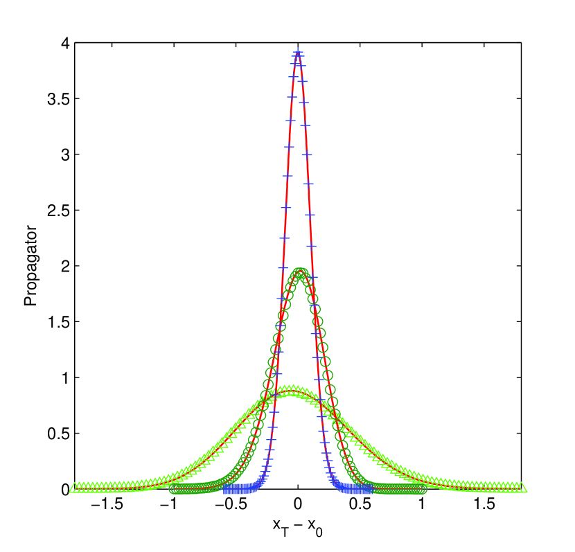
Figure 1: Propagator $\mathcal{P}(x_{T}|x_{0},\zeta_{0})$ as a function of $x_{T}-x_{0}$. The full curves are our analytical results, while the symbols represent Monte Carlo simulations. $T$ = 0.25y, $\rho$ = 0 (crosses). $T$ = 1y, $\rho$ = -0.5 (circles). $T$ = 5y, $\rho$ = 0.5 (triangles). For the other parameters the following values are used for the three figures: $\beta=5,\bar{a}=-1.6,\gamma=0.5,r=0.015$.

The goodness of this approximative propagator needs the support from MC simulations because of the lack of a closed form solution.

Figure 1 shows the propagators as a function of $x_{T}-x_{0}$, i.e., $\ln\frac{S_{T}}{S_{0}}$. The full curves come from expression (29), while the marked ones are MC simulation results, with time to maturity ranging from three months to five years, and correlation coefficients $0$, $-0.5$ and $0.5$ respectively. Here and in the rest of the article we will set $\sigma_{0}$ equal to the long time average of the volatility:

$$\sigma_{0}=\lim\limits_{t\rightarrow\infty}\mathbb{E}\left[\sigma(t)\right]=\exp\left\{\bar{a}+\frac{\gamma^{2}}{4\beta}\right\},$$ (32)

which seems a reasonable choice. For these MC simulations 5,000,000 sample paths are used.

It is seen that our analytical results fit the MC simulations quite well. Actually, using the parameters of Fig. 1, and putting expression (29) for those three cases into the left hand side of the Kolmogorov backward equation:

$$-\frac{\partial\mathcal{P}}{\partial T} + \left[r-\frac{1}{2}\,e^{2(\zeta_{0}+\bar{a})}\right]\frac{\partial\mathcal{P}}{\partial x_{0}}+\frac{1}{2}\,e^{2(\zeta_{0}+\bar{a})}\frac{\partial^{2}\mathcal{P}}{\partial x_{0}^{2}}$$

$$-\beta\zeta_{0}\frac{\partial\mathcal{P}}{\partial\zeta_{0}} + \frac{1}{2}\gamma^{2}\frac{\partial^{2}\mathcal{P}}{\partial\zeta_{0}^{2}}+\rho\,e^{\zeta_{0}+\bar{a}}\gamma\frac{\partial^{2}\mathcal{P}}{\partial x_{0}\zeta_{0}}=0,$$ (33)

we find that, for different $x_{T}$ values, the absolute values are all in the order of $10^{-7}$ or even smaller. In section IV.2 we come back to the discussion concerning the goodness of our approximation.

According to the discussion of Section II, an extension of this model to the one with price jumps is straightforward: the new marginal probability distribution would be:

$$\mathcal{P}_{LNJ}(x_{T}|0,\zeta_{0})$$ (34)

$$= \int_{-\infty}^{+\infty}\frac{dp}{2\pi}e^{ip\left[x_{T}-x_{0}-rT\right]+B\left(e^{\zeta_{0}}-1\right)}$$

$$\times e^{\frac{\beta\zeta_{0}^{2}-\omega\left(\zeta_{0}+\frac{\gamma^{2}M}{\omega^{2}}\right)^{2}}{2\gamma^{2}}+\left[\frac{\beta-\omega-A+B\gamma^{2}}{2}+\frac{\gamma^{2}M^{2}}{2\omega^{2}}\right]T}$$

$$\times\frac{e^{\frac{\Xi}{\gamma^{2}\left[2\omega+\left(\beta-\omega+B\gamma^{2}\right)(1-e^{-2\omega T})\right]}}}{\sqrt{1+\frac{1-e^{-2\omega T}}{2\omega}\left[\beta-\omega+B\gamma^{2}\right]}}$$

$$\times e^{\lambda T\int_{-\infty}^{+\infty}\left[e^{-ipJ}-1+ip\left(e^{J}-1\right)\right]\varpi(J)dJ},$$

where the same notations as in Eq.(29) are used.

IV European Vanilla Option Pricing

IV.1 General Pricing Formulas

If we denote the general marginal propagator by

$$\mathcal{P}(x_{T}|x_{0},\sigma_{0})=\int_{-\infty}^{+\infty}\frac{dp}{2\pi}\,e^{ip(x_{T}-x_{0}-rT)}F(p,T)\,e^{U(p,T)},$$ (35)

then the option pricing formula of a vanilla call option $\mathcal{C}$ with expiration date $T$ and strike price $K$ is given by the discounted expectation value of the payoff:

$$\mathcal{C} = e^{-rT}\int_{-\infty}^{+\infty}\left(e^{x_{T}}-K\right)_{+}\mathcal{P}(x_{T}|x_{0},\sigma_{0})dx_{T}$$ (36)

$$= \frac{\mathcal{G}(0)}{2}+i\int_{-\infty}^{+\infty}\frac{dp}{2\pi}\frac{e^{ip\left(\ln\frac{K}{S_{0}}-rT\right)}\mathcal{G}(p)}{p},$$

where

$$\mathcal{G}(p) = S_{0}F(p+i,T)\,e^{U(p+i,T)}$$ (37)

$$-K\,e^{-rT}F(p,T)\,e^{U(p,T)},\$$

and $\left(x\right)_{+}=\max\left(x,0\right)$.

Here we have followed the derivation outlined in Ref. Kleinert2 . In particular for the LN model $F(p,T)$ equals:

$$F(p,T) = e^{\frac{\beta\zeta_{0}^{2}-\omega\left(\zeta_{0}+\frac{\gamma^{2}M}{\omega^{2}}\right)^{2}}{2\gamma^{2}}+\left[\frac{\beta-\omega-A+B\gamma^{2}}{2}+\frac{\gamma^{2}M^{2}}{2\omega^{2}}\right]T}$$ (38)

$$\times\frac{e^{B(e^{\zeta_{0}}-1)+\frac{\Xi}{\gamma^{2}\left[2\omega+\left(\beta-\omega+B\gamma^{2}\right)(1-e^{-2\omega T})\right]}}}{\sqrt{1+\frac{1-e^{-2\omega T}}{2\omega}\left[\beta-\omega+B\gamma^{2}\right]}}.$$

At this stage one needs to specify the PDF for the jump sizes. Merton Merton and Kou Kou proposed a normal distributed jump size, denoted by $\varpi_{M}(J)$, and a asymmetric double exponential distributed one, denoted by $\varpi_{K}(J)$, respectively:

$$\varpi_{M}(J) = \frac{1}{\sqrt{2\pi\delta^{2}}}\,e^{-\frac{(J-\nu)^{2}}{2\delta^{2}}},$$ (39)

$$\varpi_{K}(J) = p_{+}\frac{1}{\eta_{+}}\,e^{-\frac{1}{\eta_{+}}J}\Theta\left(J\right)$$ (40)

$$+\,p_{-}\frac{1}{\eta_{-}}\,e^{\frac{1}{\eta_{-}}J}\,\Theta\left(-J\right).$$

For the Merton model $\nu$ is the mean jump size and $\delta$ is the standard deviation of the jump size. For Kou’s model $0<\eta_{+}<1$, $\eta_{-}>0$ are means of positive and negative jumps respectively. $p_{+}$ and $p_{-}$ represent the probabilities of positive and negative jumps, $p_{+}>0$, $p_{-}>0$, $p_{+}+$ $p_{-}=1$ and $\Theta$ is the Heaviside function.

According to expression (12), it is easy to derive their corresponding $U(p,T)$’s:

$$U_{M}(p,T) = \lambda T\left[e^{-ip\nu-\frac{1}{2}\delta^{2}p^{2}}-1\right.$$ (41)

$$\quad\quad\left.+ip\left(e^{\nu+\frac{1}{2}\delta^{2}}-1\right)\right],$$

$$U_{K}(p,T) = \lambda T\left[\frac{p_{+}}{1+ip\eta_{+}}+\frac{p_{-}}{1-ip\eta_{-}}-1\right.$$ (42)

$$\quad\quad\left.+ip(\frac{p_{+}}{1-\eta_{+}}+\frac{p_{-}}{1+\eta_{-}}-1)\right].$$

Using expression (38) and results (41), (42) in formulas (36), (37) allows to find the price of the vanilla call option for the exponential Vasicek stochastic volatility with price jumps model.

IV.2 Monte Carlo simulations

To test our analytical pricing formula for the LN model, we focus on the parameters that most strongly influence the approximation. To satisfy the assumption that quadratic fluctuations around the mean reversion level $\bar{a}$ captures the behavior of the volatility well, the mean reversion speed $\beta$ and the volatility $\gamma$ of asset volatility are crucial.

The substitution $\tau=\gamma^{2}t$ transforms expression (18) into

$$dz(\tau)=\frac{\beta}{\gamma^{2}}\left[\bar{a}-z(\tau)\right]d\tau+dB_{2}(\tau),\\$$ (43)

showing that it is actually the parameter $c=\frac{\beta}{\gamma^{2}}$ which determines whether the approximation will be good. For bigger $c$ values the approximation $z\left(t\right)\approx\bar{a}$ will be better.

As the correlation parameter $\rho$ controls the skewness of spot returns, we will also consider the typical negative and positive skewed cases by taking values $-0.5$, $0$ and $0.5$ for this parameter. On the other hand, the constant interest rate $r$ and the mean reversion level $\bar{a}$ do not influence the accuracy of the result a lot, and we just assume them to be constant values: $r=0.015$ and $\bar{a}=-1.6\approx\ln 0.2$. These two parameters seem to be quite reasonable for the present European options.

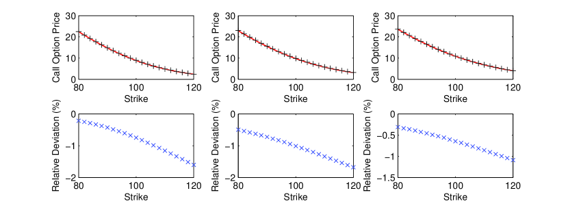
Figure 2: The upper figures show European call option prices in the LN model (left), the LN model with Merton’s jump (middle) and the LN model with Kou’s jump (right). The red curves are our analytical results and the black crosses are the Monte Carlo simulations. The corresponding lower figures give the relative deviations of our analytical results from the MC simulations in the unit of percent. Parameter values $S_{0}=100$, $r=0.015$, $T=1$, $\beta=5$, $\bar{a}=-1.6$, $\gamma=0.5$, $\rho=-0.5$, $\lambda=10$, $\nu=-0.01$, $\delta=0.03$, $p_{+}=0.3$, $p_{-}=0.7$, $\eta_{+}=0.02$, $\eta_{-}=0.04$ are used here.

To get an idea of what is a reasonable range for $c$, and since calibration values for the LN model are not available, we took calibration values from the literature Heston ; Yacine for the Heston model and fitted our model to the volatility distribution of the Heston model with those parameters. For Heston  we obtained $c\approx 7$ and for Yacine $c\approx 18$. Therefore in Table I we used values for $\beta$ and $\gamma$ such that $c$ ranges from $4.08$ up to $25$. We calculated prices for $S_{0}=100$ and $K=90,$ $100$ and $110$.

The comparison of our analytical solution with the MC solution for a European call option in the LN model as shown in Table 1 suggests that for the above mentioned parameter values the relative errors are less than $3\%$ and most of the time even less than $1\%$, which is acceptable when we take the typical bid-ask spread for European options into account. Here each MC simulation runs 20,000,000 times.

For the basic LN model we can conclude that we found an approximation valid up to $3\%$ for parameter values $c>7$ (We only checked values of $c<25$, but for bigger $c$ the approximation will only become better), $-0.5<\rho<0.5$, $T<1$ and $0.9<K/S_{0}<1.1$.

Finally we consider the vanilla call option pricing in LN model combined with Merton’s and Kou’s jumps, respectively. Since the jump process is independent from the approximation we made, we do not investigate the goodness of our approximation as thoroughly as in the basic LN model (assuming that, if it is good there it will be good here). Figure 2 illustrates our analytical results (curves) and the MC simulations (crosses), as well as the relative errors in the unit of percent. Each MC simulation runs 300,000,000 times. These results suggest that the approximation error is typically less than $2\%$. And due to the fact that whenever the degree of moneyness (the ratio of the strike price $K$ to the initial asset price $S_{0}$) is relatively high, the average bid-ask spread tends to be relatively high for call options Pena , our analytical results can serve as an easy way to get a quick estimate that is normally accurate enough for many practical applications.

V Conclusion

We presented a method which makes it possible to extend the propagator for a general SV model to the propagator of that SV model extended with an arbitrary jump process in the asset price evolution. This procedure, applied to the Heston model, leads to similar results as those obtained in Ref. Sepp , which gives us confidence in the present treatment. The stationary volatility distribution of the Heston model, however, does not correspond to the observed lognormal distribution Liu ; Micciche ; Straeten in the market. The exponential Vasicek model does have the lognormal distribution as its stationary distribution. Therefore we used this model for the volatility to illustrate the method presented in section II. For this model no closed form pricing formulas for the propagator or vanilla option prices exist. We first derive approximative formulas for the propagator and vanilla option prices for this model without jumps, using path integral methods. This result was checked with a Monte Carlo simulation, proving a parameter range for which the approximation is valid. We specified a parameter range for which our pricing formulas are accurate to within $3\%$. They become more accurate in the limit $\frac{\beta}{\gamma^{2}}>>1$ where $\beta$ is the mean reversion rate and $\gamma$ is the volatility of the volatility. Finally we extended this result to the case where the asset price evolution contains jumps.

*

Appendix A Derivation of equations (11), (12).

The proof starts by assuming that a solution for $\mathcal{P}_{J}(x_{T},\sigma_{T},T|x_{0},\sigma_{0},0)$ of the form (11) exists. Below we show that this assumption indeed leads to a solution, which in turn justifies the assumption. Since $\int_{-\infty}^{+\infty}\frac{dp}{2\pi}e^{ip(x_{T}-x_{0})}\frac{\partial F(\sigma_{T},\sigma_{0},r,p,T)}{\partial T}$ equals the right hand side of Eq.(4) and the derivative operators $\frac{\partial}{\partial x_{T}}$ and $\frac{\partial}{\partial\sigma_{T}}$ have no effect on $e^{U(p,T)}$, it follows that:

$$\frac{\partial}{\partial x_{T}}\left[-\left(r-\frac{1}{2}\sigma_{T}^{2}\right)\mathcal{P}_{J}\right]$$ (44)

$$+\frac{1}{2}\frac{\partial^{2}}{\partial x_{T}^{2}}\left[\sigma_{T}^{2}\mathcal{P}_{J}\right]+\frac{\partial}{\partial\sigma_{T}}\left[-A(T,\sigma_{T})\mathcal{P}_{J}\right]$$

$$+\frac{1}{2}\frac{\partial^{2}}{\partial\sigma_{T}^{2}}\left[B^{2}(T,\sigma_{T})\mathcal{P}_{J}\right]$$

$$+\rho\frac{\partial^{2}}{\partial x_{T}\,\partial\sigma_{T}}\left[\sigma_{T}B(T,\sigma_{T})\mathcal{P}_{J}\right]$$

$$= \int_{-\infty}^{+\infty}\frac{dp}{2\pi}e^{ip(x_{T}-x_{0})}\frac{\partial F(\sigma_{T},\sigma_{0},r,p,T)}{\partial T}\,e^{U(p,T)}.$$

Adding the term $\lambda m^{j}\frac{\partial}{\partial x_{T}}\mathcal{P}_{J}$, which is given by

$$\lambda\int_{-\infty}^{+\infty}\frac{dp}{2\pi}ip\,e^{ip(x_{T}-x_{0})}F(\sigma_{T},\sigma_{0},r,p,T)\,e^{U(p,T)}$$

$$\times\int_{-\infty}^{+\infty}(e^{J}-1)\varpi(J)dJ,$$ (45)

as well as the term $\lambda\int_{-\infty}^{+\infty}\left[\mathcal{P}_{J}(x_{T}-J)-\mathcal{P}_{J}(x_{T})\right]\varpi(J)dJ$, which is given by

$$\lambda\int_{-\infty}^{+\infty}\frac{dp}{2\pi}e^{ip(x_{T}-x_{0})}F(\sigma_{T},\sigma_{0},r,p,T)\,e^{U(p,T)}$$

$$\times\int_{-\infty}^{+\infty}\left(e^{-ipJ}-1\right)\varpi(J)dJ,$$ (46)

the right hand side of Eq.(9) is expressed as

$$\int_{-\infty}^{+\infty}\frac{dp}{2\pi}e^{ip(x_{T}-x_{0})}\frac{\partial F(\sigma_{T},\sigma_{0},r,p,T)}{\partial T}\,e^{U(p,T)}$$ (47)

$$+ \int_{-\infty}^{+\infty}\frac{dp}{2\pi}e^{ip(x_{T}-x_{0})}F(\sigma_{T},\sigma_{0},r,p,T)\,e^{U(p,T)}$$

$$\times\lambda\int_{-\infty}^{+\infty}\left[e^{-ipJ}-1+ip(e^{J}-1)\right]\varpi(J)dJ.$$

This, of course should equal the left hand side of Eq.(9), which is given by

$$\int_{-\infty}^{+\infty}\frac{dp}{2\pi}e^{ip(x_{T}-x_{0})}\frac{\partial F(\sigma_{T},\sigma_{0},r,p,T)}{\partial T}\,e^{U(p,T)}$$ (48)

$$+ \int_{-\infty}^{+\infty}\frac{dp}{2\pi}e^{ip(x_{T}-x_{0})}F(\sigma_{T},\sigma_{0},r,p,T)\frac{\partial e^{U(p,T)}}{\partial T}.$$

Expression (47) equals (48) when

$$\frac{\partial U(p,T)}{\partial T}=\lambda\int_{-\infty}^{+\infty}\left[e^{-ipJ}-1+ip\left(e^{J}-1\right)\right]\varpi(J)dJ,$$ (49)

from which the result (12) for $U(p,T)$ follows.

Table 1: Comparison of our approximative analytic pricing result and the MC simulation value for the LN model.

Parameter values
						Relative error
$K$	$\rho$	$\gamma$	$\beta$	MC value(a)	Approx.(b)	(b - a)/a (%)
90	-0.5	1.2	7	15.3947	15.2533	-0.9185
			8	15.2979	15.1731	-0.8166
			10	15.1630	15.0588	-0.6869
		0.8	5	15.1079	14.9995	-0.7180
			6	15.0307	14.9337	-0.6475
			7	14.9776	14.8855	-0.6151
	0	0.7	2	15.2486	15.1982	-0.3307
			3	15.0259	15.0024	-0.1564
			4	14.9190	14.8992	-0.1328
		0.5	1	15.2061	15.1576	-0.3187
			2	14.9030	14.8882	-0.0996
			3	14.7951	14.7865	-0.0577
	0.5	0.3	1	14.6051	14.5035	-0.6953
			1.5	14.5524	14.4815	-0.4872
			2	14.5354	14.4775	-0.3986
		0.2	0.5	14.6015	14.5398	-0.4192
			0.75	14.5609	14.5098	-0.3519
			1	14.5332	14.4981	-0.2418
100	-0.5	1.2	7	9.4541	9.2862	-1.7762
			8	9.3720	9.2197	-1.6253
			10	9.2599	9.1274	-1.4310
		0.8	5	9.1537	9.0346	-1.3006
			6	9.0950	8.9869	-1.1886
			7	9.0557	8.9534	-1.1291
	0	0.7	2	9.5394	9.4975	-0.4395
			3	9.2906	9.2704	-0.2174
			4	9.1682	9.1513	-0.1840
		0.5	1	9.4915	9.4493	-0.4480
			2	9.1445	9.1328	-0.1285
			3	9.0235	9.0155	-0.0887
	0.5	0.3	1	9.0168	8.9081	-1.2051
			1.5	8.9302	8.8522	-0.8737
			2	8.8886	8.8246	-0.7195
		0.2	0.5	8.9655	8.9023	-0.7048
			0.75	8.9039	8.8509	-0.5955
			1	8.8628	8.8247	-0.4295
110	-0.5	1.2	7	5.2749	5.1365	-2.6237
			8	5.2209	5.0916	-2.4758
			10	5.1507	5.0335	-2.2756
		0.8	5	5.0170	4.9219	-1.8947
			6	4.9877	4.8986	-1.7862
			7	4.9709	4.8849	-1.7307
	0	0.7	2	5.6480	5.5989	-0.8694
			3	5.3942	5.3705	-0.4394
			4	5.2684	5.2503	-0.3429
		0.5	1	5.5967	5.5510	-0.8173
			2	5.2475	5.2343	-0.2519
			3	5.1253	5.1160	-0.1821
	0.5	0.3	1	5.3151	5.2095	-1.9860
			1.5	5.2048	5.1289	-1.4589
			2	5.1427	5.0812	-1.1966
		0.2	0.5	5.2170	5.1576	-1.1380
			0.75	5.1449	5.0954	-0.9620
			1	5.0960	5.0595	-0.7163

Other parameter values $S_{0}=100$, $r=0.015$, $\bar{a}=-1.6$ and $T=1$ are used here.

References

• (1) F. Black and M. Scholes, Journal of Political Economy, 81, 637 (1973).
• (2) R. C. Merton, Bell Journal of Economics, 4, 141 (1973).
• (3) E. Derman and I. Kani, RISK, 7, 32 (1994).
• (4) S. Heston, Review of Financial Studies, 6, 327 (1993).
• (5) A. White and J. Hull, Journal of Finance, 42, 281 (1987).
• (6) E. Stein and J. Stein, Review of Financial Studies, 4, 727 (1991).
• (7) K. Amin and V. Ng, Journal of Finance, 48, 881 (1993).
• (8) G. Bakshi and Z. Chen, Journal of Fianancial Economics, 44, 123 (1997).
• (9) D. Lemmens, M. Wouters, J. Tempere and S. Foulon, Physical Review E, 78, 016101 (2008).
• (10) L. O. Scott, Mathematical Finance, 7, 413 (1997).
• (11) D. Duffie, J. Pan and K. Singleton, Econometrica, 68, 1343 (2000).
• (12) S. G. Kou, Management Science, 48, 1086 (2002).
• (13) R. C. Merton, Journal of Financial Economics, 3, 125 (1976).
• (14) P. Carr, H. Geman, D. B. Madan and M. Yor, Mathematical Finance 13, 345 (2003).
• (15) R. Cont and P. Tankov, Financial Modelling With Jump Processes (Chapman & Hall/CRC, 2004).
• (16) H. Geman, D. B. Madan and M. Yor, Mathematical Finance, 11, 79 (2001).
• (17) A. E. Kyprianou and W. Schoutens, P. Wilmott, Exotic Option Pricing and Advanced Levy Models (Wiley, England, 2005).
• (18) W. Schoutens, Levy processes in Finance: Pricing Financial Derivatives (Wiley, New York, 2003).
• (19) T. G. Andersen, L. Benzoni and J. Lund, Journal of Finance, 57, 1239 (2002).
• (20) D. Bates, Review of Financial Studies, 9, 69 (1996).
• (21) C. Cao, G. Bakshi and Z. Chen, Journal of Finance, 52, 2003 (1997).
• (22) M. Chernov, A. R. Gallant, E. Ghysels and G. Tauchen, Journal of Econometrics, 116, 225 (2003).
• (23) B. Eraker, M. Johannes and N. Polson, Journal of Finance, 58, 1269 (2003).
• (24) J. Pan, Journal of Financial Econometrics, 63, 3 (2002).
• (25) A. Sepp, Journal of Computational Finance, 11, 33-70 (2008).
• (26) J. Gatheral, The Volatility Surface: A Practitioner’s Guide (Wiley, 2006).
• (27) G. Yan and F. B. Hanson, Option Pricing for a Stochastic-Volatility Jump-Diffusion Model with Log-Uniform Jump-Amplitudes, Proceedings of the 2006 American Control Conference.
• (28) Y. Liu, P. Gopikrishnan, P. Cizeau, M. Meyer, C. Peng and H. E. Stanley, Physical Review E, 60, 1390 (1999).
• (29) S. Micciche, G. Bonanno, F. Lillo and R. N. Mantegna, Physica A, 314, 756 (2002).
• (30) B. E. Baaquie, Quantum finance: Path Integrals and Hamiltonians for Options and Interest Rates (Cambridge University Press, Cambridge, 2004).
• (31) H. Kleinert, Path Integrals in Quantum Mechanics, Statistics, Polymer Physics, and financial Markets (Word Scientific, Singapore, 2009).
• (32) J. W. Dash, Quantitative Finance and Risk Management: A Physicist’s Approach (World Scientific, Singapore, 2004).
• (33) E. Van der Straeten and C. Beck, Physical Review E, 80, 036108 (2009).
• (34) J. Voit, The Statistical Mechanics of Financial Markets (Springer, 2005).
• (35) C. W. Gardiner, Handbook of Stochastic Methods (Springer, 2004).
• (36) M. Chesney and L. Scott, Journal of Financial and Quantitative Analysis, 24, 267 (1989).
• (37) P. Nozieres and S. Schmitt-Rink, J. Low Temp. Phys. 59, 195 (1985).
• (38) C. A. R. Sa de Melo, M. Randeria, and J. R. Engelbrecht, Phys. Rev. Lett. 71, 3202 (1993).
• (39) H. Kleinert, Physica A, 338, 151 (2004).
• (40) Y. Aït-Sahalia and R. Kimmel, Journal of Financial Economics, 83, 413 (2007).
• (41) I. Pena, G. Rubio and G. Serna, European Financial Management, 7, 351 (2001).