Interacting Multiple Try Algorithms with Different Proposal Distributions

Abstract

We propose a new class of interacting Markov chain Monte Carlo (MCMC) algorithms designed for increasing the efficiency of a modified multiple-try Metropolis (MTM) algorithm. The extension with respect to the existing MCMC literature is twofold. The sampler proposed extends the basic MTM algorithm by allowing different proposal distributions in the multiple-try generation step. We exploit the structure of the MTM algorithm with different proposal distributions to naturally introduce an interacting MTM mechanism (IMTM) that expands the class of population Monte Carlo methods. We show the validity of the algorithm and discuss the choice of the selection weights and of the different proposals. We provide numerical studies which show that the new algorithm can perform better than the basic MTM algorithm and that the interaction mechanism allows the IMTM to efficiently explore the state space.

1 Introduction

Markov chain Monte Carlo (MCMC) algorithms are now essential for the analysis of complex statistical models. In the MCMC universe, one of the most widely used class of algorithms is defined by the Metropolis-Hastings (MH) (Metropolis et al., 1953; Hastings, 1970) and its variants. An important generalization of the standard MH formulation is represented by the multiple-try Metropolis (MTM) (Liu et al., 2000). While in the MH formulation one accepts or rejects a single proposed move, the MTM is designed so that the next state of the chain is selected among multiple proposals. The multiple-proposal setup can be used effectively to explore the sample space of the target distribution and subsequent developments made use of this added flexibility. For instance, Craiu and Lemieux (2007) propose to use antithetic and quasi-Monte Carlo samples to generate the proposals and to improve the efficiency of the algorithm while Pandolfi et al. (2010b) and Pandolfi et al. (2010a) apply the multiple-proposal idea to a trans-dimensional setup and combine Reversible Jump MCMC with MTM.

This work further generalizes the MTM algorithm presented in Liu et al. (2000) in two directions. First, we show that the original MTM transition kernel can be modified to allow for different proposal distributions in the multiple-try generation step while preserving the ergodicity of the chain. The use of different proposal distributions gives more freedom in designing MTM algorithms for target distributions that require different proposals across the sample space. An important challenge remains the choice of the distributions used to generate the proposals and we propose to address it by expanding upon methods used within the population Monte Carlo class of algorithms.

The class of population Monte Carlo procedures (Cappé et al., 2004; Del Moral and Miclo, 2000; Del Moral, 2004; Jasra et al., 2007) has been designed to address the inefficiency of classical MCMC samplers in complex applications involving multimodal and high dimensional target distributions (Pritchard et al., 2000; Heard et al., 2006). Its formulation relies on a number of MCMC processes that are run in parallel while learning from one another about the geography of the target distribution.

A second contribution of the paper is finding reliable generic methods for constructing the proposal distributions for the MTM algorithm.We propose an interacting MCMC sampling design for the MTM that preserves the Markovian property. More specifically, in the proposed interacting MTM (IMTM) algorithm, we allow the distinct proposal distributions to use information produced by a population of auxiliary chains. We infer that the resulting performance of the MTM is tightly connected to the performance of the chains’ population. In order to maximize the latter, we propose a number of strategies that can be used to tune the auxiliary chains. We also adapt previous extensions of the MTM and link the use of stochastic overrelaxation, random-ray Monte Carlo method (see Liu et al., 2000) and simulated annealing to IMTM.

In the next section we discuss the IMTM algorithm, propose a number of alternative implementations and prove their ergodicity. In Section 3 we focus on some special cases of the IMTM algorithm and in Section 4 the performance of the methods proposed is demonstrated with simulations and real examples. We end the paper with a discussion of future directions for research.

2 Interacting Monte Carlo Chains for MTM

We begin by describing the MTM and its extension for using different proposal distributions.

2.1 Multiple-Try Metropolis With Different Proposal Distributions

Suppose that of interest is sampling from a distribution $\pi$ that has support in $\mathcal{Y}\subset{\mathbf{R}}^{d}$ and is known up to a normalizing constant. Assuming that the current state of the chain is $x$, the update defined by the MTM algorithm of Liu et al. (2000) is described in Algorithm 1.

 

Algorithm 1.

Multiple-try Metropolis Algorithm (MTM)

 

1. Draw $M$ trial proposals $y_{1},\ldots,y_{M}$ from the proposal distribution $T(\cdot|x)$. Compute $w(y_{j},x)$ for each $j\in\{1,\ldots,M\}$, where $w(y,x)=\pi(y)T(x|y)\lambda(y,x),$ and $\lambda(y,x)$ is a symmetric function of $x,y$.

2. Select $y$ among the $M$ proposals with probability proportional to $w(y_{j},x),j=1,\ldots,M$.

3. Draw $x_{1}^{*},\ldots,x_{M-1}^{*}$ variates from the distribution $T(\cdot|y)$ and let $x_{M}^{*}=x$.

4. Accept $y$ with generalized acceptance probability

   $$\rho=\min\left\{1,\frac{w(y_{1},x)+\ldots+w(y_{M},x)}{w(x_{1}^{*},y)+\ldots+w(x_{M}^{*},y)}\right\}.$$

 

Note that while the MTM uses the same distribution to generate all the proposals, it is possible to extend this formulation to different proposal distributions without altering the ergodicity of the associated Markov chain.

Let $T_{j}(x,\cdot)$, with $j=1,\ldots,M$, be a set of proposal distributions for which $T_{j}(x,y)>0$ if and only if $T_{j}(y,x)>0$. Define

$$w_{j}(x,y)=\pi(x)T_{j}(x,y)\lambda_{j}(x,y)\qquad j=1,\ldots,M$$

where $\lambda_{j}(x,y)$ is a nonnegative symmetric function in $x$ and $y$ that can be chosen by the user. The only requirement is that $\lambda_{j}(x,y)>0$ whenever $T(x,y)>0$. Then the MTM algorithm with different proposal distributions is given in Algorithm 2.

 

Algorithm 2.

MTM with Different Proposal Distributions

 

1. Draw independently $M$ proposals $y_{1},\ldots,y_{M}$ such that $y_{j}\sim T_{j}(x,\cdot)$. Compute $w_{j}(y_{j},x)$ for $j=1,\ldots,M$.

2. Select $Y=y$ among the trial set $\{y_{1},\ldots,y_{M}\}$ with probability proportional to $w_{j}(y_{j},x)$, $j=1,\ldots,M$. Let $J$ be the index of the selected proposal. Then draw $x_{j}^{*}\sim T_{j}(y,\cdot)$, $j\neq J$, $j=1,\ldots,M$ and let $x_{J}^{*}=x$.

3. Accept y with probability

   $$\rho=\min\left\{1,\frac{w_{1}(y_{1},x)+\cdots+w_{M}(y_{M},x)}{w_{1}(x_{1}^{*},y)+\cdots+w_{M}(x_{M}^{*},y)}\right\}$$

   and reject with probability $1-\rho$.

 

It should be noted that Algorithm 2 is a special case of the interacting MTM presented in the next section and that the proof of ergodicity for the associated chain follows closely the proof given in Appendix A for the interacting MTM and is not given here.

In Section 4 we will show, through simulation experiments, that this algorithm is more efficient then a MTM algorithm with a single proposal distribution.

2.2 General Construction

Undoubtedly, Algorithm 2 offers additional flexibility in organizing the MTM sampler. This section introduces generic methods for using a population of MCMC chains to define the proposal distributions.

 

Algorithm 3.

Interacting Multiple Try Algorithm (IMTM)

 

• For $i=1,\ldots,N$

  1. Let $x=x_{n}^{(i)}$, for $j=1,\ldots,M_{i}$ draw $y_{j}\sim T_{j}^{(i)}(\cdot|x_{n}^{(1:i-1)},x,x_{n}^{(i+1:N)})$ independently and compute

     $$w_{j}^{(i)}(y_{j},x)=\pi(y_{j})T_{j}^{(i)}(y_{j}|x_{n}^{(1:i-1)},x,x_{n}^{(i+1:N)})\lambda_{j}^{(i)}(y_{j},x).$$

  2. Select $J\in\{1,\ldots,M_{i}\}$ with probability proportional to $w_{j}^{(i)}(y_{j},x)$, $j=1,\ldots,M_{i}$ and set $y=y_{J}$.

  3. For $j=1,\ldots,M_{i}$ and $j\neq J$ draw $x_{j}^{*}\sim T_{j}^{(i)}(\cdot|x_{n}^{(1:i-1)},y,x_{n}^{(i+1:N)})$, let $x_{J}^{*}=x_{n}^{(i)}$ and compute

     $$w_{j}^{(i)}(x_{j}^{*},y)=\pi(x_{j}^{*})T_{j}^{(i)}(x_{j}^{*}|x_{n}^{(1:i-1)},y,x_{n}^{(i+1:N)})\lambda_{j}^{(i)}(x_{j}^{*},y).$$

  4. Set $x_{n+1}^{(i)}=y$ with probability

     $$\rho_{i}=\min\left\{1,\frac{w_{1}^{(i)}(y_{1},x)+\ldots+w_{M_{i}}^{(i)}(y_{M_{i}},x)}{w_{1}^{(i)}(x_{1}^{*},y)+\ldots+w_{M_{i}}^{(i)}(x_{M_{i}}^{*},y)}\right\}$$

     and $x_{n+1}^{(i)}=x_{n}^{(i)}$ with probability $1-\rho_{i}$.

 

Consider a population of $N$ chains, $X^{(i)}=\{x_{n}^{(i)}\}_{n\in\mathbb{N}}$ and $i=1,\ldots,N$. For full generality we assume that the $i$th chain has MTM transition kernel with $M_{i}$ different proposals $\{T_{j}^{(i)}\}_{1\leq j\leq M_{i}}$ (if we set $M_{i}=1$ we imply that the chain has a MH transition kernel). The interacting mechanism allows each proposal distribution to possibly depend on the values of the chains at the previous step. Formally, if $\Xi_{n}=\{x_{n}^{(i)}\}_{i=1}^{N}$ is the vector of values taken at iteration $n\in\mathbb{N}$ by the population of chains, then we allow each proposal distribution used in updating the population at iteration $n+1$ to depend on $\Xi_{n}$. The mathematical formalization is used in the description of Algorithm 3. One expects that the chains in the population are spread throughout the sample space and thus the proposals generated are a good representation of the sample space ${\cal{Y}}$ ultimately resulting in better mixing for the chain of interest.

In order to give a representation of the IMTM transition density let us introduce the following notation. Let $T_{j}^{(i)}(x,y)=T_{j}^{(i)}(y|x_{n}^{(1:i-1)},x,x_{n}^{(i+1:N)})$, $T^{(i)}(x,y_{1:M_{i}})=\prod_{k=1}^{M_{i}}T_{k}^{(i)}(x,y_{k})$ and $T_{-j}^{(i)}(x,y_{1:M_{i}})=\prod_{k\neq j}^{M_{i}}T_{k}^{(i)}(x,y_{k})$ and define $dy_{1:M_{i}}=\prod_{k=1}^{M_{i}}dy_{k}$ and $dy_{-j}=\prod_{k\neq j}^{M_{i}}dy_{k}$.

The transition density associated to the population of chains is then

$$K(\Xi_{n},\Xi_{n+1})=\prod_{i=1}^{N}K_{i}(x_{n}^{(i)},x_{n+1}^{(i)})$$ (1)

where

$$K_{i}(x,y)=\sum_{j=1}^{M_{i}}A_{j}^{(i)}(x,y)T_{j}^{(i)}(x,y)+\left(1-\sum_{j=1}^{M_{i}}B_{j}^{(i)}(x)\right)\delta_{x}(y)$$ (2)

is the transition kernel associated to the $i$-th chain of algorithm with

$$A_{j}^{(i)}(x,y)=\int_{\mathcal{Y}^{2(M_{i}-1)}}\tilde{w}_{j}^{(i)}(y,x)\rho_{j}^{(i)}(x,y)T_{-j}^{(i)}(y,x^{*}_{1:M_{i}})T_{-j}^{(i)}(x,y_{1:M_{i}})dx^{*}_{-j}dy_{-j}$$

and

$$B^{(i)}_{j}(x)=\int_{\mathcal{Y}^{2(M_{i}-1)+1}}\rho_{j}^{(i)}(x,y)T_{-j}^{(i)}(y,dx^{*}_{1:M_{i}})T^{(i)}(x,dy_{1:M_{i}})dx^{*}_{-j}dy_{1:M_{i}}.$$

In the above equations $\tilde{w}_{j}^{(i)}(y_{j},x)=w_{j}^{(i)}(y_{j},x)/(w_{j}^{(i)}(y,x)+\bar{w}_{-k}^{(i)}(y_{1:M_{i}}|x))$, with $j=1,\ldots,M_{i}$ and $\bar{w}_{-j}^{(i)}(y_{1:M_{i}}|x)=$ $\sum_{k\neq j}^{M_{i}}w_{k}^{(i)}(y_{k},x)$, are the normalized weights used in the selection step of the IMTM algorithm and

$$\rho_{j}^{(i)}(x,y)=\min\left\{1,\frac{w_{j}^{(i)}(y,x)+\bar{w}_{-j}^{(i)}(y_{1:M_{i}}|x)}{w_{j}^{(i)}(x,y)+\bar{w}_{-j}^{(i)}(x_{1:M_{i}}^{*}|y)}\right\}$$

is the generalized MH ratio associated to a MTM algorithm.

The validity of Algorithm 3 relies upon the detailed balance condition.

Theorem 1.

The transition density $K_{i}(x_{n}^{(i)},x_{n+1}^{(i)})$ associated to the $i$-th chain of the IMTM algorithm satisfies the conditional detailed balanced condition.

Proof

See Appendix A.

Since the transition $K_{i}(x_{n}^{(i)},x_{n+1}^{(i)})$, $i=1,\ldots,N$ has $\pi(x)$ as stationary distribution and satisfies the conditional detailed balance condition then the joint transition $K(\Xi_{n},\Xi_{n+1})$ has $\pi(x)^{N}$ as a stationary distribution.

An important issue directly connected to the practical implementation of the IMTM is the choice of proposal distributions and the choice of $\lambda_{j}^{(i)}(x,y)$. First it should be noted that at each iteration of the interacting chains the computational complexity of the algorithm is $\mathcal{O}(N\sum_{i=1}^{N}M_{i})$. When considering the number of chains and the number of proposals, there are two possible strategies in designing the interaction mechanism.

The first strategy is to use a small number of chains, say $2\leq N\leq 5$, in order to improve the mixing of each chain and to allow for large jumps between different regions of the state space. When applying this strategy to our IMTM algorithms it is possible to set the number of proposals to be equal to the number of chains, i.e. $M_{i}=N$, for all $1\leq i\leq N$. In this way all the chains can interact at each iteration of the algorithm and many search directions can be included among the proposals.

A second strategy is to use a higher number of chains, e.g. $N=100$, in order to possibly have, at each iteration, a good approximation of the target or a much higher number of search directions for a good exploration of the sample space. This algorithm design strategy is common in Population Monte Carlo or Interacting MCMC methods. Clearly when a high number of chains is used within IMTM, it is necessary to set $M_{i}<N$. In the next section we discuss a few strategies to built the $M_{i}$ proposals.

2.3 Parsing the Population of Auxiliary Chains

One of the strategies that revealed to be successful in our applications consists in the random selection of a certain number of chains of the population in order to build the proposals. More specifically, we let $M_{i}=M$, for all $i$, and when updating the $i$-th chain of the population we sample $I_{1},\ldots,I_{M}$ random indexes from the uniform distribution $\mathcal{U}_{\{1,\ldots,N\}}$, with $N>M$, and then set the proposals: $T_{j}^{(i)}(y,x)=T_{j}^{(i)}(\cdot|x,x_{n}^{(I_{1})},\ldots,x_{n}^{(I_{M})})$, for all $j=1,\ldots,M$. On the basis of our simulation experiments we found that the following choice $T_{j}^{(i)}(\cdots|x_{n}^{(I_{1})},\ldots,x_{n}^{(I_{M})})=T_{j}(\cdot|x_{n}^{(I_{j})})$ is works well in improving the mixing of the chains.

Previously suggested forms for the function $\lambda_{j}^{(i)}(x,y)$ (Liu et al., 2000) are:

1. $\lambda_{j}^{(i)}(x,y)=1$

2. $\lambda_{j}^{(i)}(x,y)=2\{T_{j}^{(i)}(x,y)+T_{j}^{(i)}(y,x)\}^{-1}$

3. $\lambda_{j}^{(i)}(x,y)=\{T_{j}^{(i)}(x,y)T_{j}^{(i)}(y,x)\}^{-\alpha}$, $\alpha>0$.

Here we propose to include in the choice of $\lambda$ the information provided by the population of chains. Therefore we suggest to modify the above functions as follows

1. $\lambda_{j}^{(i)}(x,y)=\nu_{j}$

2. $\lambda_{j}^{(i)}(x,y)=2\nu_{j}\,\{T_{j}^{(i)}(x,y)+T_{j}^{(i)}(y,x)\}^{-1}$

3. $\lambda_{j}^{(i)}(x,y)=\nu_{j}\,\{T_{j}^{(i)}(x,y)T_{j}^{(i)}(y,x)\}^{-\alpha}$, $\alpha>0$

where the factor $\nu_{j}$ captures the behaviour of the auxiliary chains at the previous iteration

$$\nu_{j}=\frac{1}{N}\sum_{i=1}^{N}\mathbb{I}_{\{j\}}(J_{n-1}^{(i)}),\quad j=1,\ldots,M$$

where $J_{n-1}^{(i)}$ is the random index of the selection step at the iteration $n-1$ for the $i$-th chain. The modifications proposed for $\lambda(\cdot,\cdot)$ would increase the use of those proposal distributions favoured by the population of chains at previous iteration. Since $\nu_{j}$ depends only on samples generated at the previous step by the population of chains, the ergodicity of the IMTM chain is preserved. An alternative strategy is to sample the random indexes $I_{1},\ldots,I_{M}$ with probabilities proportional to $\nu_{j}$.

2.4 Annealed IMTM

Our belief in IMTM’s improved performance is underpinned by the assumption that the population of Monte Carlo chains is spread throughout the sample space. This can be partly achieved by initializing the chains using draws from a distribution overdispersed with respect to $\pi$ (see also Jennison, 1993; Gelman and Rubin, 1992) and partly by modifying the stationary distribution for some of the chains in the population. Specifically, we consider the sequence of annealed distributions $\pi_{t}=\pi^{t}$ with $t\in\{\xi_{1},\xi_{2},\ldots,\xi_{N}\}$, where $1=\xi_{1}>\xi_{2}>\ldots>\xi_{n}$, for instance $\xi_{t}=1/t$. When $t,s$ are close temperatures, $\pi_{t}$ is similar to $\pi_{s}$, but $\pi=\pi_{1}$ may be much harder to sample from than $\pi_{\xi_{N}}$ as has been long recognized in the simulated annealing and simulated tempering literature (see Marinari and Parisi, 1992; Geyer and Thompson, 1994; Neal, 1994). Therefore, it is likely that some of the chains designed to sample from $\pi_{1},\ldots,\pi_{N}$ have good mixing properties, making them good candidates for the population of MCMC samplers needed for the IMTM.

We thus consider the Monte Carlo population made of the $N-1$ chains having $\{\pi_{2},\ldots,\pi_{N}\}$ as stationary distributions. An example of annealed interacting MTM is given in Algorithm 4. Note that we let the $i$-th chain to interact only with the $N-i+1$ chains at higher temperature by sampling $I_{1},\ldots,I_{M}$ from $\mathcal{U}_{\{1,\ldots,N-i+1\}}$.

An astute reader may have noticed that the use of MTM for each auxiliary chain may be redundant since for smaller $\xi_{i}$’s the distribution $\pi_{i}$ is easy to sample from. In Algorithm 5 we present an alternative implementation of the annealed IMTM in which each auxiliary chain is MH with target $\pi_{i}$, $1\leq i\leq N-1$.

 

Algorithm 4.

Annealed IMTM Algorithm (AIMTM1)

 

• For $i=1,\ldots,N$

  1. Let $x=x_{n}^{(i)}$ and sample $I_{1},\ldots,I_{M}$ from $\mathcal{U}_{\{1,\ldots,N-i+1\}}$.

  2. For $j=1,\ldots,M$ draw $y_{j}\sim T_{j}^{(i)}(\cdot|x_{n}^{(I_{j})})$ independently and compute

     $$w_{j}^{(i)}(y_{j},x)=\pi(y_{j})T_{j}^{(i)}(y_{j}|x_{n}^{(I_{j})})\lambda_{j}^{(i)}(y_{j},x).$$

  3. Select $J\in\{1,\ldots,M\}$ with probability proportional to $w_{j}^{(i)}(y_{j},x)$, $j=1,\ldots,M$ and set $y=y_{J}$.

  4. For $j=1,\ldots,M$ and $j\neq J$ draw $x_{j}^{*}\sim T_{j}^{(i)}(\cdot|x_{n}^{(1:i-1)},y,x_{n}^{(i+1:N)})$, let $x_{J}^{*}=x_{n}^{(i)}$ and compute

     $$w_{j}^{(i)}(x_{j}^{*},y)=\pi(x_{j}^{*})T_{j}^{(i)}(x_{j}^{*}|y)\lambda_{j}^{(i)}(x_{j}^{*},y).$$

  5. Set $x_{n+1}^{(i)}=y$ with probability $\rho_{i}$, where $\rho_{i}$ is the generalized M.H. ratio of the IMT algorithm and $x_{n+1}^{(i)}=x_{n}^{(i)}$ with probability $1-\rho_{i}$.

 

 

Algorithm 5.

Annealed IMTM Algorithm (AIMTM2)

 

• For $i=1$

  1. Let $x=x_{n}^{(i)}$ and sample $I_{1},\ldots,I_{M}$ from $\mathcal{U}_{\{1,\ldots,N\}}$.

  2. For $j=1,\ldots,M$ draw $y_{j}\sim T_{j}^{(i)}(\cdot|x_{n}^{(I_{j})})$ independently and compute

     $$w_{j}^{(i)}(y_{j},x)=\pi(y_{j})T_{j}^{(i)}(y_{j}|x_{n}^{(I_{j})})\lambda_{j}^{(i)}(y_{j},x).$$

  3. Select $J\in\{1,\ldots,M\}$ with probability proportional to $w_{j}^{(i)}(y_{j},x)$, $j=1,\ldots,M$ and set $y=y_{J}$.

  4. For $j=1,\ldots,M$ and $j\neq J$ draw $x_{j}^{*}\sim T_{j}^{(i)}(\cdot|x_{n}^{(1:i-1)},y,x_{n}^{(i+1:N)})$, let $x_{J}^{*}=x_{n}^{(i)}$ and compute

     $$w_{j}^{(i)}(x_{j}^{*},y)=\pi(x_{j}^{*})T_{j}^{(i)}(x_{j}^{*}|y)\lambda_{j}^{(i)}(x_{j}^{*},y).$$

  5. Set $x_{n+1}^{(i)}=y$ with probability $\rho_{i}$, where $\rho_{i}$ is the generalized M.H. ratio of the IMT algorithm and $x_{n+1}^{(i)}=x_{n}^{(i)}$ with probability $1-\rho_{i}$.

• For $i=2,\ldots,N$

  1. Let $x=x_{n}^{(i)}$ and update the proposal function $T^{(i)}(\cdot|x)$.

  2. Draw $y\sim T^{(i)}(\cdot|x)$ and compute

     $$\rho_{i}=\min\left\{1,\frac{\pi(y)^{\xi_{i}}T^{(i)}(x|y)}{\pi(x)^{\xi_{i}}T^{(i)}(y|x)}\right\}.$$

  3. Set $x_{n+1}^{(i)}=y$ with probability $\rho_{i}$ and $x_{n+1}^{(i)}=x_{n}^{(i)}$ with probability $1-\rho_{i}$.

 

The chain of interest, corresponding to $\xi=1$, has an MTM transition kernel with $M=N-1$ proposal distributions. At time $n$ the $j$th proposal distribution used for the chain ergodic to $\pi$ is $T_{j}^{(1)}=T^{(j)}$, is the same as the proposal used by the $j$th auxiliary chain, for all $2\leq j\leq N$.

An additional gain could be obtained if the auxiliary chains’ transition kernels are modified using adaptive MCMC strategies (see also Chauveau and Vandekerkhove, 2002, for another example of adaption for interacting chains). However, it should be noted that letting the auxiliary chains adapt indefinitely results in complex theoretical justifications for the IMTM which go beyond the scope of this paper and will be presented elsewhere. Our current recommendation is to use finite adaptation for the auxiliary chains prior to the start of the IMTM. One could take advantage of multi-processor computing units and use parallel programming to increase the computational efficiency of this approach.

The adaptation of $\lambda^{(i)}_{j}(\cdot,\cdot)$, through the weights $\nu_{j}$ defined in the previous section, should be used cautiously in this case. The aim of the annealing procedure is to allow the higher temperatures chains to explore widely the sample space and to improve the mixing of the MTM chain. Using $\nu_{j}$ the context of annealed IMTM could arbitrarily penalize some of the higher temperature proposals and reduce the effectiveness of the annealing strategy.

It is possible to have a Monte Carlo approximation of a quantity of interest by using the output produced by all the chains in the population. For example let

$$\mathcal{I}=\int_{\mathcal{Y}}h(x)\pi(x)dx$$

be the quantity of interest where $h$ is a test function. It is possible to approximate this quantity as follows

$$\mathcal{I}_{NT}=\frac{1}{T}\sum_{n=1}^{T}\frac{1}{\bar{\zeta}}\sum_{j=1}^{N}h(x_{n}^{(j)})\zeta_{j}(x_{n}^{(j)})$$

where $x_{n}^{(i)}$, with $n=1,\ldots,T$ and $i=1,\ldots,N$ is the output of a IMTM chains with target $\pi^{\xi_{i}}$ and $\zeta_{j}(x)=\pi(x)/\pi^{\xi_{j}}(x)$ is a set of importance weights with normalizing constant $\bar{\zeta}=\sum_{j=1}^{N}\zeta_{j}(x_{n}^{(j)})$.

2.5 Gibbs within IMTM update

It should be noticed that in the proposed algorithm at the $n$-th iteration the $N$ chains are updated simultaneously. In the interacting MCMC literature a sequential updating scheme (Gibbs-like updating) has been proposed for example in Mengersen and Robert (2003) and Campillo et al. (2009). In the following we show that the Gibbs-like updating also apply to our IMTM context. In the Gibbs-like interacting MTM (GIMTM) algorithm given in Algorithm 6 the different proposals functions of the $i$-th chain, with $i=1,\ldots,N$, may depend on the current values of the updated chains $x_{n+1}^{(j)}$, with $j=1,\ldots,(i-1)$ and on the last values $x_{n}^{(j)}$, with $j=(i+1),\ldots,N$, of the chains which have not yet been updated.

 

Algorithm 6.

Gibbs-like IMTM Algorithm (GIMTM)

 

• For $i=1,\ldots,N$

  1. For $j=1,\ldots,M_{i}$ draw $y_{j}\sim T_{j}^{(i)}(\cdot|x_{n+1}^{(1:i-1)},x_{n}^{(i)},x_{n}^{(i+1:N)})$ independently and compute

     $$w_{j}^{(i)}(y_{j},x)=\pi(y_{j})T_{j}^{(i)}(y_{j}|x_{n+1}^{(1:i-1)},x_{n}^{(i)},x_{n}^{(i+1:N)})\lambda_{j}^{(i)}(y_{j},x_{n}^{(i)}).$$

  2. Select $J\in\{1,\ldots,M_{i}\}$ with probability proportional to $w_{j}^{(i)}(y_{j},x)$, $j=1,\ldots,M_{i}$ and set $y=y_{J}$.

  3. For $j=1,\ldots,M_{i}$ and $j\neq J$ draw $x_{j}^{*}\sim T_{j}^{(i)}(\cdot|x_{n+1}^{(1:i-1)},y,x_{n}^{(i+1:N)})$, let $x_{J}^{*}=x_{n}^{(i)}$ and compute

     $$w_{j}^{(i)}(x_{j}^{*},y)=\pi(x_{j}^{*})T_{j}^{(i)}(x_{j}^{*}|x_{n+1}^{(1:i-1)},y,x_{n}^{(i+1:N)})\lambda_{j}^{(i)}(x_{j}^{*},y).$$

  4. Set $x_{n+1}^{(i)}=y$ with probability

     $$\rho_{i}=\min\left\{1,\frac{w_{1}^{(i)}(y_{1},x)+\ldots+w_{M_{i}}^{(i)}(y_{M_{i}},x)}{w_{1}^{(i)}(x_{1}^{*},y)+\ldots+w_{M_{i}}^{(i)}(x_{M_{i}}^{*},y)}\right\}$$

     and $x_{n+1}^{(i)}=x_{n}^{(i)}$ with probability $1-\rho_{i}$.

 

In the GIMTM algorithm the iteration mechanism between the chains is not the same as in the IMTM algorithm. The chains are no longer independent since the proposals may depend on the current values for some of the chains in the population. The transition kernel for the whole population is

$$K(\Xi_{n},\Xi_{n+1})=\prod_{i=1}^{N}K_{i}(x_{n}^{(i)},x_{n+1}^{(i)}|x_{n+1}^{(1:i-1)},x_{n}^{(i+1:N)})$$

and in this case the validity of the algorithm still relies upon the conditional detail balance condition given for the IMTM algorithm.

Finally we remark that the GIMTM algorithm allows us to introduce further possible choices for the $\lambda_{j}^{(i)}(x,y)$ functions. In particular a repulsive factor (see Mengersen and Robert (2003)) can be introduced in the selection weights in order to induce negative dependence between the chains. We let the study of the GIMTM algorithm and the use of repulsive factors for future research and focus instead on the properties of the IMTM algorithm.

3 Some generalizations

In the following we will discuss some possible generalization of the IMTM algorithm. First we show how to use the stochastic overrelaxation method to possibly have a further gain in the efficiency. Secondly we suggest two possible strategies to built the different proposal functions of the IMTM. The first strategy consists in proposing values along different search directions and represents an extension of the random-ray Monte Carlo algorithm presented in Liu et al. (2000). The second strategy relies upon a suitable combination of target tempering and adaptive MCMC chains.

3.1 Stochastic Overrelaxation

Stochastic overrelaxation (SOR) is a Markov chain Monte Carlo technique developed by Adler (1981) for normal densities and subsequently extended by Green and Han (1992) for non-normal targets. The idea behind this approach is to induce negative correlation between consecutive draws of a single MCMC process.

Within the MTM algorithm we can implement SOR by inducing negative correlation between the proposals and between the proposals and the current state of the chain, $x$. A natural and easy to implement procedure may be based on the assumption that $(y_{1},\ldots,y_{M-1},x)^{T}\sim N_{d\times M}(\mathbf{0},V)$ where $V$’s structure is dictated by the desired negative dependence between the proposals $y_{1},\ldots,y_{n}$’s and $x$, specifically

$$V=\left(\begin{array}[]{cccc}\Sigma_{1}&\Psi_{12}&\ldots&\Psi_{1M}\\ \Psi_{12}&\Sigma_{2}&\ldots&\Psi_{2M}\\ \ldots&\ldots&\ldots&\ldots\\ \Psi_{1M}&\Psi_{2M}&\ldots&\Sigma_{M}\\ \end{array}\right).$$

For instance, we can set $\Psi_{ij}=0$ whenever $i,j\neq M$ and $\Psi_{iM}=\Sigma_{i}^{1/2}R_{iM}\Sigma_{M}^{1/2}$ where $R_{iM}$ is a correlation matrix which corresponds to extreme negative correlation (see Craiu and Meng, 2005, for a discussion of extreme dependence) between any two components (with same index) of $y_{i}$ and $x$, for any $1\leq i\leq M-1$. The general construction falls within the context of dependent proposals as discussed by Craiu and Lemieux (2007) with the additional bonus of ”pulling” the proposals away from the current state due to the imposed negative correlation. This essentially ensures that no proposals are exceedingly close to the current location of the chain. Also note that the construction is general enough and can be applied for Algorithms 2 and 3 as long as the proposal distributions are Gaussian.

3.2 Multiple Random-ray Monte Carlo

We show here that the use of different proposals for the MTM algorithm allows also to extend the random-ray Monte Carlo method given in Liu et al. (2000). In particular the proposed algorithm allows to deal with multiple search directions at each iteration of the chains. At the $n$-th iteration of the chain, in order to update the set of chains $\Xi_{n}$, the algorithm performs for each chain $x_{n}^{(r)}\in\Xi_{n}$, with $r=1,\ldots,N$, the following steps:

1. Evaluate the gradient $\log\pi(x)$ at $x_{n}^{(r)}$ and find the mode $a_{n}$ along $x_{n}^{(r)}+ru_{n}$ where $u_{n}=x_{n}^{(r)}-x_{n-1}^{(r)}$.

2. Sample $I_{1},\ldots,I_{M}$ from the uniform $\mathcal{U}_{\{1,\ldots,r-1,r+1,\ldots,N\}}$.

3. Let $e_{n,j}=(a_{n}-x_{n}^{(I_{j})})/||a_{n}-x_{n}^{(I_{j})}||$ and sample $r_{j}$ from $\mathcal{N}(0,\sigma^{2})$.

and then use the set of proposals $T_{j}$ which depends on $e_{n,j}$ to perform a MTM transition with different proposals as in the IMTM algorithm (see Alg. 1).

4 Simulation Results

4.1 Single-chain results

In this section we carry out, through some examples, a comparison between the single-chain multiple try algorithms MTM-DP with different proposals and the algorithm in Liu et al. (2000). In the MTM-DP algorithm we consider four Gaussian random-walk proposals $\mathbf{y}_{j}\sim\mathcal{N}_{n}(\mathbf{x},\Lambda_{j})$ with $\Lambda_{1}=0.1Id_{n}$, $\Lambda_{2}=5Id_{n}$, $\Lambda_{3}=50Id_{n}$ and $\Lambda_{4}=100Id_{n}$, where $Id_{n}$ denotes the $n$-order identity matrix. In the MTM selection weights we set $\lambda_{j}(\mathbf{x},\mathbf{y})=2\alpha_{j}/(T_{j}(\mathbf{x},\mathbf{y})+T_{j}(\mathbf{y},\mathbf{x}))$, where $\alpha_{j}=0.25$, for $j=1,\ldots,4$.

In order to compare the MTM algorithm with different proposals and the Multiple Try algorithm of Liu et al. (2000) we consider 20,000 iterations and use four trials $\mathbf{y}_{j}$ generated by the following proposal

$$T_{j}(\mathbf{x},\mathbf{y}_{j})=\sum_{j=1}^{4}\alpha_{j}\mathcal{N}_{n}(\mathbf{x},\Lambda_{j})$$ (3)

where $\Lambda_{j}$, $j=1,\ldots,4$, have been defined above. In the weighs of the selection step we set $\lambda(\mathbf{x},\mathbf{y})=2/(T_{j}(\mathbf{x},\mathbf{y})+T_{j}(\mathbf{y},\mathbf{x}))$.

4.1.1 Bivariate Mixture with two components

We consider the following bivariate mixture of two normals

$$\frac{1}{3}\mathcal{N}_{2}(\boldsymbol{\mu}_{1},\Sigma_{1})+\frac{2}{3}\mathcal{N}_{2}(\boldsymbol{\mu}_{2},\Sigma_{2})$$ (4)

with $\boldsymbol{\mu}_{1}=(0,0)^{\prime}$, $\boldsymbol{\mu}_{2}=(10,10)^{\prime}$, $\Sigma_{1}=\hbox{diag}(0.1,0.5)$ and $\Sigma_{2}=\hbox{diag}(0.5,0.1)$.

In Fig. 1 the ACF with 30 lags for the first component of the bivariate MH chain. The autocorrelation is lower for the MTM algorithm with different proposals.

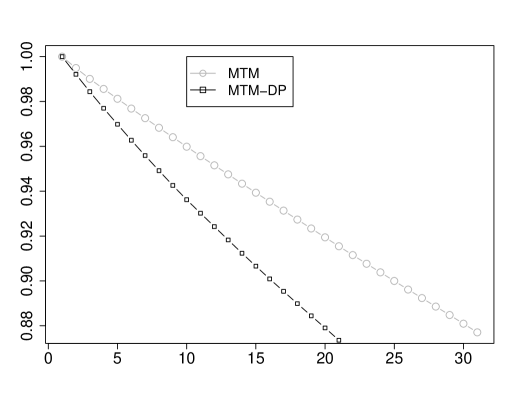
Figure 1: Autocorrelation function of the Liu’s MTM (gray line) and MTM with different proposals (black line).

Figure 2: Autocorrelation function (ACF) of the 20 components of the multivariate MH chain for the Liu’s MTM (gray lines) and MTM with different proposals (black lines).

4.1.2 Multivariate Normal Mixture

We compare the algorithms for high-dimensional targets. We consider the following multivariate mixture of two normals with a sparse variance-covariance structure

$$\frac{1}{3}\mathcal{N}_{20}(\boldsymbol{\mu}_{1},\Sigma_{1})+\frac{2}{3}\mathcal{N}_{20}(\boldsymbol{\mu}_{2},\Sigma_{2})$$ (5)

with $\boldsymbol{\mu}_{1}=(3,\ldots,3)^{\prime}$, $\boldsymbol{\mu}_{2}=(10,\ldots,10)^{\prime}$ and $\Sigma_{j}$, with $j=1,2$, generated independently from a Wishart distribution $\Sigma_{j}\sim\mathcal{W}_{20}(\nu,Id_{20})$ where $\nu$ is the degrees of freedom parameter of the Wishart. In the experiments we set $\nu=21$.

The autocorrelation function of the chain for one of the experiment is given in Fig. 2. The ACF has been evaluated for each components of the $20$-dimensional chain. The values of the ACF of the MTM-DP (black lines in Fig. 2) are less than those of the original MTM (gray lines of the same figure) in all the directions of the support space. We conclude that the MTM algorithm with different proposals (Algorithm 3) outperforms the Liu et al. (2000) MTM algorithm.

4.2 Multiple-chains results

In this section we show real and simulated data results of the general interacting multiple try algorithm in Alg. 1.

4.2.1 Bivariate Mixture with two components

The target distribution is the following bivariate mixture of two normals

$$\frac{1}{3}\mathcal{N}_{2}(\boldsymbol{\mu}_{1},\Sigma_{1})+\frac{2}{3}\mathcal{N}_{2}(\boldsymbol{\mu}_{2},\Sigma_{2})$$ (6)

with $\boldsymbol{\mu}_{1}=(0,0)^{\prime}$, $\boldsymbol{\mu}_{2}=(10,10)^{\prime}$, $\Sigma_{1}=\hbox{diag}(0.1,0.5)$ and $\Sigma_{2}=\hbox{diag}(0.5,0.1)$.

We consider a population of $N=50$ chains with $M=50$ proposals and 1,000 iterations of the IMTM algorithm. For each chain we consider the case $T_{j}^{(i)}(\mathbf{y}|\mathbf{x}_{n+1}^{(1:i-1)},\mathbf{x}_{n}^{(i)},\mathbf{x}_{n}^{(i+1:N)})=T^{(j)}(\mathbf{y},\mathbf{x}_{n}^{(j)})$ and draw

$$\mathbf{y}_{j}\sim\mathcal{N}_{2}(\mathbf{x}_{n}^{(j)},\Lambda_{j})$$ (7)

where $\Lambda_{j}=(0.1+5j)Id_{2}$. In this specification of the IMTM algorithm each chain has $M$ independent proposals with conditional mean given by the previous values of the chains in the population.

In this experiment we consider two kind of weights. First we set $\lambda_{j}^{(i)}(x,y)=(T_{j}^{(i)}(x,y)T_{j}^{(i)}(y,x))^{-1}$, that corresponds to use importance sampling selection weights, secondly we consider $\lambda_{j}^{(i)}(x,y)=2(T_{j}^{(i)}(x,y)+T_{j}^{(i)}(y,x))^{-1}$, which implies a symmetric MTM algorithm. We denote with IMTM-IS and IMTM-TA respectively the resulting algorithms.

Fig. 3 show the results of the IMTM-IS and IMTM-TA algorithms at the last iteration of the population of chains (black dots). In both of the algorithms the population is visiting the two modes of the distribution in the right proportion. Moreover each chain is able to jump from one mode to the other. (the light-gray line represents the sample path of one of the chain).

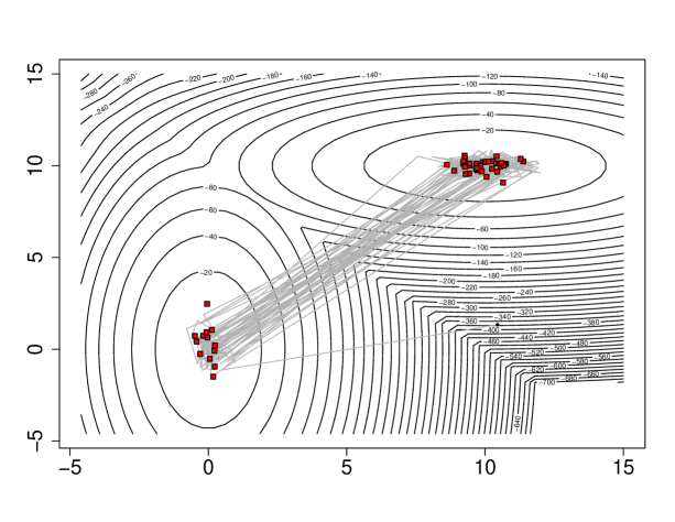
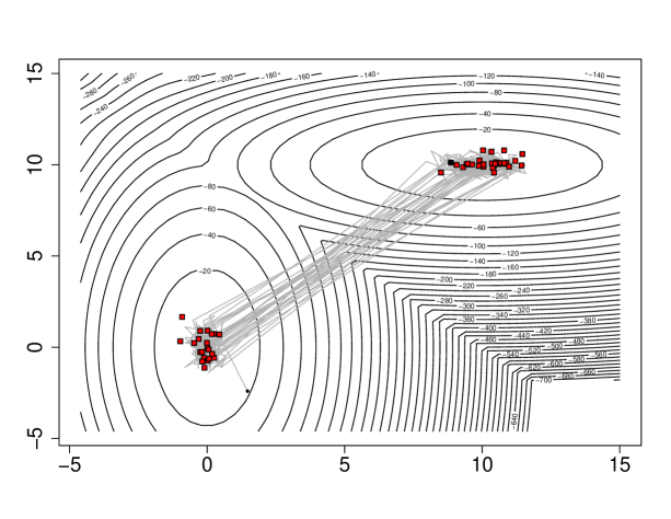
Figure 3: Log-target level sets (solid lines), the MH chains (red dots) at the last iteration of the IMTM algorithms and the path of one of the chain of the set (gray line). Up: output of the IMTM-IS with importance sampling selection weights. Bottom: ouput of the IMTM-TA with symmetric lambda as in (c).

4.2.2 Beta-Binomial Model

We consider here the problem of the genetic instability of esophageal cancers. During a neoplastic progression the cancer cells undergo a number of genetic changes and possibly lose entire chromosome sections. The loss of a chromosome section containing one allele by abnormal cells is called Loss of Heterozygosity (LOH). The LOH can be detected using laboratory assays on patients with two different alleles for a particular gene. Chromosome regions containing genes which regulate cell behavior, are hypothesized to have a high rates of LOH. Consequently the loss of these chromosome sections disables important cellular controls.

Chromosome regions with high rates of LOH are hypothesized to contain Tumor Suppressor Genes (TSGs), whose deactivation contributes to the development of esophageal cancer. Moreover the neoplastic progression is thought to produce a high level of background LOH in all chromosome regions.

In order to discriminate between ”background” and TSGs LOH, the Seattle Barrett’s Esophagus research project (Barrett et al. (1996)) has collected LOH rates from esophageal cancers for 40 regions, each on a distinct chromosome arm. The labeling of the two groups is unknown so Desai (2000) suggest to consider a mixture model for the frequency of LOH in both the ”background” and TSG groups.

We consider the hierarchical Beta-Binomial mixture model proposed in Warnes (2001)

$$f(x,n|\eta,\pi_{1},\pi_{2},\gamma)=\eta{n\choose x}\pi_{1}^{x}(1-\pi_{1})^{n-x}+$$ (8)

$$\quad(1-\eta){n\choose x}\frac{\Gamma(1/\omega_{2})}{\Gamma(\pi_{2}/\omega_{2})\Gamma((1-\pi_{2})/\omega_{2})}\frac{\Gamma(x+\pi_{2}/\omega_{2})\Gamma(n-x+(1-\pi_{2})/\omega_{2})}{\Gamma(n+1/\omega_{2})}$$

with $x$ number of LOH sections, $n$ the number of examined sections, $\omega_{2}=\exp\{\gamma\}/(2(1+\exp\{\gamma\}))$. Let $\mathbf{x}=(x_{1},\ldots,x_{m})$ and $\mathbf{n}=(n_{1},\ldots,n_{m})$ be a set of observations from $f(x,n|\eta,\pi_{1},\pi_{2},\gamma)$ and let us assume the following priors

$$\eta\sim\mathcal{U}_{[0,1]},\quad\pi_{1}\sim\mathcal{U}_{[0,1]},\quad\pi_{2}\sim\mathcal{U}_{[0,1]}\quad\hbox{and}\quad\gamma\sim\mathcal{U}_{[-30,30]}$$ (9)

with $\mathcal{U}$ the uniform distribution on $[a,b]$. Then the posterior distribution is

$$\pi(\eta,\pi_{1},\pi_{2},\gamma|\mathbf{x},\mathbf{n})\propto\prod_{j=1}^{m}f(x_{j},n_{j}|\eta,\pi_{1},\pi_{2},\gamma)$$ (10)

The parametric space is of dimension four: $(\eta,\pi_{1},\pi_{2},\gamma)\in[0,1]^{3}\times[-30,30]$ and the posterior distribution has two well-separated modes making it difficult to sample using generic methods.

Figure 4: Values of the population of chains (dots) at the last iteration on the subspace ($\pi_{1}$,$\pi_{2}$). The interaction is given by $M=4$ proposal functions randomly selected between the population of $N=100$ chains.

We apply the IMTM algorithm with $100$ iterations, $M=4$ proposal functions randomly selected between a population of $N=100$ chains. For each chain we consider importance sampling weights in the selection step, i.e. we set $\lambda_{j}^{(i)}(x,y)=(T_{j}^{(i)}(x,y)T_{j}^{(i)}(y,x))^{-1}$ with $j=1,\ldots,4$ and $i=1,\ldots,100$. The values of the population of chains (dots) at the last iteration on the subspace ($\pi_{1}$,$\pi_{2}$) is given in Fig. 4. The IMTM is able to visit both regions of the parameter space confirming the analysis of Craiu et al. (2009) and Warnes (2001).

4.2.3 Stochastic Volatility

The estimation of the stochastic volatility (SV) model due to Taylor (1994) still represents a challenging issue in both off-line (Celeux et al. (2006)) and sequential (Casarin and Marin (2009)) inference contexts. One of the main difficulties is due to the high dimension of the sampling space which hinders the use of the data-augmentation and prevents a reliable joint estimation of the parameters and the latent variables. As highlighted in Casarin et al. (2009) using multiple chains with a chain interaction mechanism could lead to a substantial improvement in the MCMC method for this kind of model. We consider the SV model given in Celeux et al. (2006)

$$y_{t}|h_{t} \sim \mathcal{N}\left(0,e^{h_{t}}\right)$$

$$h_{t}|h_{t-1},\boldsymbol{\theta} \sim \mathcal{N}\left(\alpha+\phi h_{t-1},\sigma^{2}\right)$$

$$h_{0}|\boldsymbol{\theta} \sim \mathcal{N}\left(0,\sigma^{2}/(1-\phi^{2})\right)$$

with $t=1,\ldots,T$ and $\boldsymbol{\theta}=$ $(\alpha$, $\phi$, $\sigma^{2})$. For the parameters we assume the noninformative prior (see Celeux et al., 2006)

$$\pi(\boldsymbol{\theta})\propto 1/(\sigma\beta)\mathbb{I}_{(-1,1)}(\phi)$$

where $\beta^{2}=\exp(\alpha)$. In order to simulate from the posterior we consider the full conditional distributions and apply a Gibbs algorithm. If we define $\mathbf{y}=(y_{1},\ldots,y_{T})$ and $\mathbf{h}=(h_{0},\ldots,h_{T})$ then the full conditionals for $\beta$ and $\phi$ are the inverse gamma distributions

$$\beta^{2}|\mathbf{h},\mathbf{y}\quad \sim \mathcal{I}\mathcal{G}\left(\sum_{t=1}^{T}y^{2}_{t}\exp(-h_{t})/2,(T-1)/2\right)\,$$

$$\sigma^{2}|\phi,\mathbf{h},\mathbf{y} \sim \mathcal{I}\mathcal{G}\left(\sum_{t=2}^{T}(h_{t}-\phi h_{t-1})^{2}/2+h^{2}_{1}(1-\phi^{2}),(T-1)/2\right)$$

and $\phi$ and the latent variables have non-standard full conditionals

$$\!\!\!\!\!\!\!\!\!\pi(\phi|\sigma^{2},\mathbf{h},\mathbf{y})\propto(1-\phi^{2})^{1/2}\exp\left(-\frac{\phi^{2}}{2\sigma^{2}}\sum_{t=2}^{T-1}h^{2}_{t}-\frac{\phi}{\sigma^{2}}\sum_{t=2}^{T}h_{t}h_{t-1}\right)\mathbb{I}_{(-1,+1)}(\phi)\,$$

$$\!\!\!\!\!\!\!\!\!\pi(h_{t}|\alpha,\phi,\sigma^{2},\mathbf{h},\mathbf{y})\propto\exp\left(-\frac{1}{2\sigma^{2}}\left((h_{t}-\alpha-\phi h_{t-1})^{2}-\right.\right.$$

$$\quad\quad\quad\quad\quad\quad\quad\quad\quad\quad\left.\left.(h_{t+1}-\alpha-\phi h_{t})^{2}\right)-\frac{1}{2}\left(h_{t}+y^{2}_{t}\exp(-h_{t})\right)\right).$$

In order to sample from the posterior we use an IMTM within Gibbs algorithm. A detailed description of the proposal distributions for $\phi$ and $h_{t}$ can be found in Celeux et al. (2006).

We consider the two parameter settings $(\alpha$, $\phi$,$\,\sigma^{2})=$ $(0,0.99,0.01)$ and $(\alpha$,$\,\phi$,$\,\sigma^{2})=$ $(0,0.9,0.1)$ which correspond, in a financial stock market context, to daily and weekly frequency data respectively. Note that as reported in Casarin and Marin (2009) inference in the daily example is more difficult. We compare the performance of MH within Gibbs and IMTM within Gibbs algorithms in terms of Mean Square Error (MSE) for the parameters and of cumulative RMSE for the latent variables. We carry out the comparison in statistical terms and estimate the MSE and RMSE by running the algorithms on 20 independent simulated datasets of 200 observations. In the comparison we take into account the computational cost and for the IMTM within Gibbs we use $N=20$ interacting chains, 1,000 iterations and $M=5$ proposal functions. This setting corresponds to 100,000 random draws and is equivalent to the 100,000 iterations of the MH within Gibbs algorithm used in the comparison. Note that the proposal step of the IMTM selects at random the proposal functions between the other chains and the selection step uses $\lambda_{j}^{(i)}(x,y)=(T_{j}^{(i)}(x,y)T_{j}^{(i)}(y,x))^{-1}$, with $h=1,\ldots,5$ and $i=1,\ldots,20$.

The results for the parameter estimation when applying IMTM are presented in Table 1 and show an effective improvement in the estimates, both for weekly and daily data, when compared to the results of a MH algorithm with an equivalent computational load.

	Daily Data				Weekly Data
$\theta$	Value	MSE		$\theta$	Value	MSE
		IMTM	MH			IMTM	MH
$\alpha$	0	0.04698	0.09517	$\alpha$	0	0.00146	0.00849
		(0.00612)	(0.00194)			(0.00139)	(0.00105)
$\phi$	0.99	0.20109	0.34825	$\phi$	0.9	0.01328	0.10746
		(0.02414)	(0.05187)			(0.04014)	(0.03629)
$\sigma^{2}$	0.01	0.00718	0.02380	$\sigma^{2}$	0.1	0.00136	0.09175
		(0.00173)	(0.00202)			(0.00141)	(0.00358)

Table 1: Mean square error (MSE) and its standard deviation (in parenthesis) for the parameter estimation with IMTM and MH within Gibbs algorithms. Left panel: daily datasets. Right panel: weekly dataset.

A typical output of the IMTM for some chains of the population and for the latent variables $\mathbf{h}$ is given in Fig. 5. Each chart shows for a given chain the estimated latent variables (dotted black line), the posterior quantiles (gray lines) and the true value of $\mathbf{h}$ (solid black line).

Figures 6 and 6 exhibit the HPD region at the 90% (gray areas) and the mean (black lines) of the cumulative RMSE of each algorithm for the weekly and daily data, respectively. The statistics have been estimated from 20 independent experiments. The average RMSE shows that, in both parameter settings considered here, the IMTM (dashed black line) is more efficient than the standard MH algorithm (solid black line).

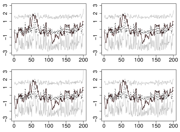
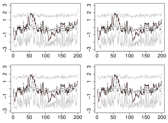
Figure 5: Typical output of the population of chains for a weekly dataset. For each chain the estimated latent variable (dotted black line), the 2.5% and 97.5% quantiles (gray lines) and the true value of $\mathbf{h}$ (solid black line).

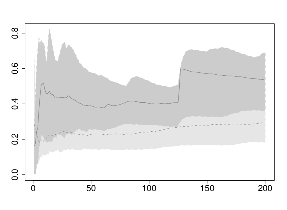
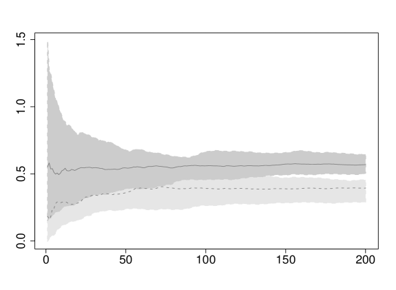
Figure 6: Cumulative RMSE for the IMTM (dashed line) and MH (solid line) and the 90% HPD regions for the IMTM (light gray) and MH (dark gray) estimated on 20 independent experiments for both the daily (up) and weekly (bottom) datasets.

5 Conclusions

In this paper we propose a new class of interacting Metropolis algorithm, with Multiple Try transition. These algorithms extend the existing literature in two directions. First we show a natural and not straightforward way to include the chains interaction in a multiple try transition. Secondly the multiple try transition has been extended in order to account for the use of different proposal functions. We give a proof of validity of the algorithm and show on real and simulated examples the effective improvement in the mixing property and exploration ability of the resulting interacting chains.

Appendix A

Proof

Without loss of generality, we drop the chain index $i$ and the iteration index $n$, set $M_{i}=N$, $\forall i$ and $x_{n}^{(i)}=x$ and denote with $T_{j}(y,x)=$ $T_{j}(y|x_{n+1}^{(1:i-1)},x_{n}^{(i)},x_{n}^{(i+1:N)})$ $\lambda_{j}^{(i)}(y_{j},x_{n}^{(i)})$ the $j$ proposal of the $i$-th chain at the iteration $n$ conditional on the past and current values, $x_{n+1}^{(1:i-1)}$ and $x_{n}^{(i+1:N)}$ respectively, of the other chains.

Let us define the following quantities

$$\bar{w}(y_{1:N}|x)=\sum_{j=1}^{N}w_{j}(y_{j},x),\quad\bar{w}_{-k}(y_{1:N}|x)=\sum_{j\neq k}^{N}w_{j}(y_{j},x)$$

and

$$S_{N}(J)=\frac{1}{\bar{w}(y_{1:N}|x)}\sum_{j=1}^{N}\delta_{j}(J)w_{j}(y_{j},x)$$

with $J\in\mathcal{J}=\{1,\ldots,N\}$ the empirical measure generated by different proposals and by the normalized selection weights.

Let $T(x,dy_{1:N})=\bigotimes_{j=1}^{N}T_{j}(x,dy_{j}):(\mathcal{Y}\times\mathcal{B}(\mathcal{Y}^{N}))\mapsto[0,1]$ the joint proposal for the multiple try and define $T_{-k}(x,dy_{1:N})=\bigotimes_{j\neq k}^{N}T_{j}(x,dy_{j})$. Let $A(x,y)$ be the actual transition probability for moving from x to y in the IMT2 algorithm. Suppose that $x\neq y$, then the transition is a results two steps. The first step is a selection step which can be written as $y=y_{J}$ and $x_{J}^{*}=x$ with the random index $J$ sampled from the empirical measure $S_{N}(J)$. The second step is a accept/reject step based on the generalized MH ratio which involves the generation of the auxiliary values $x_{j}^{*}$ for $j\neq J$. Then

$$\pi(x)A(x,y)=$$

$$=\pi(x)\int_{\mathcal{Y}^{N}}T(x,dy_{1:N})\int_{\mathcal{J}}S_{N}(dJ)\int_{\mathcal{Y}^{N-1}\times\mathcal{Y}^{2}}T_{-J}(y,dx^{*}_{1:N})\times$$

$$\quad\times\delta_{x}(dx^{*}_{J})\delta_{y_{J}}(dy)\min\left\{1,\frac{\bar{w}(y_{1:N}|x)}{\bar{w}(x_{1:N}^{*}|y)}\right\}$$

$$=\pi(x)\sum_{j=1}^{N}\int_{\mathcal{Y}^{N-1}}T_{-j}(x,dy_{1:N})T_{j}(x,y)\int_{\mathcal{Y}^{N-1}}T_{-j}(y,dx^{*}_{1:N})\times$$

$$\quad\times\frac{w_{j}(y,x)}{w_{j}(y,x)+\bar{w}_{-j}(y_{1:N}|x)}\min\left\{1,\frac{w_{j}(y,x)+\bar{w}_{-j}(y_{1:N}|x)}{w_{j}(x,y)+\bar{w}_{-j}(x_{1:N}^{*}|y)}\right\}$$

$$=\sum_{j=1}^{N}\frac{w_{j}(x,y)w_{j}(y,x)}{\lambda_{j}(y,x)}\int_{\mathcal{Y}^{2(N-1)}}T_{-j}(x,dy_{1:N})\times$$

$$\quad\times T_{-j}(y,dx^{*}_{1:N})\min\left\{\frac{1}{w_{j}(y,x)+\bar{w}_{-j}(y_{1:N}|x)},\frac{1}{w_{j}(x,y)+\bar{w}_{-j}(x_{1:N}^{*}|y)}\right\}$$

which is symmetric in x and y.

References

- Barrett et al. (1996) Barrett, M., Galipeau, P., Sanchez, C., Emond, M. and Reid, B. (1996). Determination of the frequency of loss of heterozygosity in esophageal adeno-carcinoma nu cell sorting, whole genome amplification and microsatellite polymorphisms. Oncogene 12.
- Campillo et al. (2009) Campillo, F., Rakotozafy, R. and Rossi, V. (2009). Parallel and interacting Markov chain Monte Carlo algorithm. Mathematics and Computers in Simulation 79 3424–3433.
- Cappé et al. (2004) Cappé, O., Gullin, A., Marin, J. and Robert, C. P. (2004). Population Monte Carlo. J. Comput. Graph. Statist. 13 907–927.
- Casarin and Marin (2009) Casarin, R. and Marin, J.-M. (2009). Online data processing: Comparison of Bayesian regularized particle filters. Electronic Journal of Statistics 3 239–258.
- Casarin et al. (2009) Casarin, R., Marin, J.-M. and Robert, C. (2009). A discussion on: Approximate Bayesian inference for latent Gaussian models by using integrated nested Laplace approximations by Rue, H. Martino, S. and Chopin, N. Journal of the Royal Statistical Society Ser. B 71 360–362.
- Celeux et al. (2006) Celeux, G., Marin, J.-M. and Robert, C. (2006). Iterated importance sampling in missing data problems. Computational Statistics and Data Analysis 50 3386–3404.
- Chauveau and Vandekerkhove (2002) Chauveau, D. and Vandekerkhove, P. (2002). Improving convergence of the hastings-metropolis algorithm with an adaptive proposal. Scandinavian Journal of Statistics 29 13.
- Craiu and Lemieux (2007) Craiu, R. V. and Lemieux, C. (2007). Acceleration of the multiple-try Metropolis algorithm using antithetic and stratified sampling. Statistics and Computing 17 109–120.
- Craiu and Meng (2005) Craiu, R. V. and Meng, X. L. (2005). Multi-process parallel antithetic coupling for forward and backward MCMC. Ann. Statist. 33 661–697.
- Craiu et al. (2009) Craiu, R. V., Rosenthal, J. S. and Yang, C. (2009). Learn from thy neighbor: Parallel-chain adaptive and regional MCMC. Journal of the American Statistical Association 104 1454–1466.
- Del Moral (2004) Del Moral, P. (2004). Feynman-Kac Formulae. Genealogical and Interacting Particle Systems with Applications. Springer.
- Del Moral and Miclo (2000) Del Moral, P. and Miclo, L. (2000). Branching and interacting particle systems approximations of feynmanc-kac formulae with applications to non linear filtering. In Séminaire de Probabilités XXXIV. Lecture Notes in Mathematics, No. 1729. Springer, 1–145.
- Desai (2000) Desai, M. (2000). Mixture Models for Genetic changes in cancer cells. Ph.D. thesis, University of Washington.
- Gelman and Rubin (1992) Gelman, A. and Rubin, D. B. (1992). Inference from iterative simulation using multiple sequences (with discussion). Statist. Sci. 457–511.
- Geyer and Thompson (1994) Geyer, C. J. and Thompson, E. A. (1994). Annealing Markov chain Monte Carlo with applications to ancestral inference. Tech. Rep. 589, University of Minnesota.
- Hastings (1970) Hastings, W. K. (1970). Monte Carlo sampling methods using Markov chains and their applications. Biometrika 57 97–109.
- Heard et al. (2006) Heard, N. A., Holmes, C. and Stephens, D. (2006). A quantitative study of gene regulation involved in the immune response od anophelinemosquitoes: an application of Bayesian hierarchical clustering of curves. J. Amer. Statist. Assoc. 101 18–29.
- Jasra et al. (2007) Jasra, A., Stephens, D. and Holmes, C. (2007). On population-based simulation for static inference. Statist. Comput. 17 263–279.
- Jennison (1993) Jennison, C. (1993). Discussion of ”Bayesian computation via the Gibbs sampler and related Markov chain Monte Carlo methods,” by A.F.M. Smith and G.O. Roberts. J. Roy. Statist. Soc. Ser. B 55 54–56.
- Liu et al. (2000) Liu, J., Liang, F. and Wong, W. (2000). The multiple-try method and local optimization in Metropolis sampling. Journal of the American Statistical Association 95 121–134.
- Marinari and Parisi (1992) Marinari, E. and Parisi, G. (1992). Simulated tempering: A new Monte Carlo scheme. Europhysics Letters 19 451–458.
- Mengersen and Robert (2003) Mengersen, K. and Robert, C. (2003). The pinball sampler. In Bayesian Statistics 7 (J. Bernardo, A. Dawid, J. Berger and M. West, eds.). Springer-Verlag.
- Metropolis et al. (1953) Metropolis, N., Rosenbluth, A., Rosenbluth, M., Teller, A. and Teller, E. (1953). Equations of state calculations by fast computing machines. J. Chem. Ph. 21 1087–1092.
- Neal (1994) Neal, R. M. (1994). Sampling from multimodal distributions using tempered transitions. Tech. Rep. 9421, University of Toronto.
- Pandolfi et al. (2010a) Pandolfi, S., Bartolucci, F. and Friel, N. (2010a). A generalization of the multiple-try metropolis algorithm for bayesian estimation and model selection. In 13th International Conference on Artificial Intelligence and Statistics (AIS-TATS), Chia Laguna Resort, Sardinia, Italy. ???
- Pandolfi et al. (2010b) Pandolfi, S., Bartolucci, F. and Friel, N. (2010b). A generalized Multiple-try Metropolis version of the Reversible Jump algorithm. Tech. rep., http://arxiv.org/pdf/1006.0621.
- Pritchard et al. (2000) Pritchard, J. K., Stephens, M. and Donnelly, P. (2000). Inference of population structure using multilocus genotype data. Genetics 155 945–959.
- Roberts and Rosenthal (2007) Roberts, G. O. and Rosenthal, J. S. (2007). Coupling and ergodicity of adaptive Markov chain Monte Carlo algorithms. J. Appl. Probab. 44 458–475.
- Taylor (1994) Taylor, S. (1994). Modelling stochastic volatility. Mathematical Finance 4 183–204.
- Warnes (2001) Warnes, G. (2001). The Normal kernel coupler: An adaptive Markov chain Monte Carlo method for efficiently sampling from multi-modal distributions. Technical report, George Washington University.