Santa Claus Schedules Jobs on Unrelated Machines

Abstract

One of the classic results in scheduling theory is the $2$-approximation algorithm by Lenstra, Shmoys, and Tardos for the problem of scheduling jobs to minimize makespan on unrelated machines, i.e., job $j$ requires time $p_{ij}$ if processed on machine $i$. More than two decades after its introduction it is still the algorithm of choice even in the restricted model where processing times are of the form $p_{ij}\in\{p_{j},\infty\}$. This problem, also known as the restricted assignment problem, is NP-hard to approximate within a factor less than $1.5$ which is also the best known lower bound for the general version.

Our main result is a polynomial time algorithm that estimates the optimal makespan of the restricted assignment problem within a factor $33/17+\epsilon\approx 1.9412+\epsilon$, where $\epsilon>0$ is an arbitrarily small constant. The result is obtained by upper bounding the integrality gap of a certain strong linear program, known as configuration LP, that was previously successfully used for the related Santa Claus problem. Similar to the strongest analysis for that problem our proof is based on a local search algorithm that will eventually find a schedule of the mentioned approximation guarantee, but is not known to converge in polynomial time.

1 Introduction

Scheduling on unrelated machines is the model where we are given a set $\mathcal{J}$ of jobs to be processed without interruption on a set $\mathcal{M}$ of unrelated machines, where the time a machine $i\in\mathcal{M}$ needs to process a job $j\in\mathcal{J}$ is specified by a machine and job dependent processing time $p_{ij}\geq 0$. When considering a scheduling problem the most common and perhaps most natural objective function is makespan minimization. This is the problem of finding a schedule, also called an assignment, $\sigma:\mathcal{J}\mapsto\mathcal{M}$ so as to minimize the time $\max_{i\in\mathcal{M}}\sum_{j\in\sigma^{-1}(i)}p_{ij}$ required to process all the jobs.

A classic result in scheduling theory is Lenstra, Shmoys, and Tardos’ $2$-approximation algorithm for this basic problem [13]. Their approach is based on several nice structural properties of the extreme point solutions of a natural linear program and has become a text book example of such techniques (see, e. g., [18]). Complementing their positive result they also proved that the problem is NP-hard to approximate within a factor less than $1.5$ even in the restricted case when $p_{ij}\in\{p_{j},\infty\}$ (i. e., when job $j$ has processing time $p_{j}$ or $\infty$ for each machine). This problem is also known as the restricted assignment problem and, although it looks easier than the general version, the algorithm of choice has been the same $2$-approximation algorithm as for the general version.

Despite being a prominent open problem in scheduling theory, there has been very little progress on either the upper or lower bound since the publication of [13] over two decades ago. One of the biggest hurdles for improving the approximation guarantee has been to obtain a good lower bound on the optimal makespan. Indeed, the considered linear program has been useful for generalizations such as introducing job and machine dependent costs [16, 17] but is known to have an integrality gap of $2-1/|\mathcal{M}|$ even in the restricted case. We note that Shchepin and Vakhania [15] presented a rounding achieving this gap slightly improving upon the approximation ratio of $2$.

In a relatively recent paper, Ebenlendr et al. [6] overcame this issue in the special case of the restricted assignment problem where a job can be assigned to at most two machines. Their strategy was to add more constraints to the studied linear program, which allowed them to prove a $1.75$-approximation algorithm for this special case that they named Graph Balancing. The name arises naturally when interpreting the restricted assignment problem as a hypergraph with a vertex for each machine and a hyperedge $\Gamma(j)=\{i\in\mathcal{M}:p_{ij}=p_{j}\}$ for each job $j\in\mathcal{J}$ that is incident to the machines it can be assigned to. As pointed out by the authors of [6] it seems difficult to extend their techniques to hold for more general cases. In particular, it can be seen that the considered linear program has an integrality gap of $2$ when we allow jobs that can be assigned to $3$ machines.

In this paper we overcome this obstacle by considering a certain strong linear program, often referred to as configuration LP. In particular, we obtain the first asymptotic improvement on the approximation factor of $2$.

Theorem 1.1

There is a polynomial time algorithm that estimates the optimal makespan of the restricted assignment problem within a factor of $33/17+\epsilon\approx 1.9412+\epsilon$, where $\epsilon>0$ is an arbitrarily small constant.

We note that our proof gives a local search algorithm to also find a schedule with performance guarantee $\frac{33}{17}$ but it is not known to converge in polynomial time.

Our techniques are based on the recent development on the related Santa Claus problem. In the Santa Claus problem we are given the same input as in the considered scheduling problem but instead of wanting to minimize the maximum we wish to maximize the minimum, i. e., to find an assignment $\sigma$ so as to maximize $\min_{i\in\mathcal{M}}\sum_{j\in\sigma^{-1}(i)}p_{ij}$. The playful name now follows from associating the machines with kids and jobs with presents. Santa Claus’ problem then becomes to distribute the presents so as to make the least happy kid as happy as possible.

The problem was first considered under this name by Bansal and Sviridenko [3]. They formulated and used the configuration LP to obtain an $O(\log\log\log|\mathcal{M}|/\log\log|\mathcal{M}|)$-approximation algorithm for the restricted Santa Claus problem, where $p_{ij}\in\{p_{j},0\}$. They also proved several structural properties that were later used by Feige [7] to prove that the integrality gap of the configuration LP is in fact constant in the restricted case. The proof is based on repeated use of Lovász local lemma and was only recently turned into a polynomial time algorithm [9].

The approximation guarantee obtained by combining [7] and [9] is a large constant and the techniques do not seem applicable to the considered problem. This is because the methods rely on structural properties that are obtained by rounding the input and such a rounding applied to the scheduling problem would rapidly eliminate any advantage obtained over the current approximation ratio of $2$. Instead, our techniques are mainly inspired by a paper of Asadpour et al. [1] who gave a tighter analysis of the configuration LP for the restricted Santa Claus problem. More specifically, they proved that the integrality gap is lower bounded by $1/4$ by designing a local search algorithm that eventually finds a solution with the mentioned approximation guarantee, but is not known to converge in polynomial time.

Similar to their approach, we formulate the configuration LP and show that its integrality gap is upper bounded by $33/17$ by designing a local search algorithm. As the configuration LP can be solved in polynomial time up to any desired accuracy [3], this implies Theorem 1.1. Although we cannot prove that the local search converges in polynomial time, our results imply that the configuration LP gives a polynomial time computable lower bound on the optimal makespan that is strictly better than two. We emphasize that all the results related to hardness of approximation remain valid even for estimating the optimal makespan.

Before proceeding, let us mention that unlike the restricted assignment problem, the special case of uniform machines and that of a fixed number of machines are both significantly easier to approximate and are known to admit polynomial time approximation schemes [10, 11, 12]. Also scheduling jobs on unrelated machines to minimize weighted completion time instead of makespan has a better approximation algorithm with performance guarantee $1.5$ [14]. The Santa Claus problem has also been studied under the name Max-Min Fair Allocation and there have been several recent results for the general version of the problem (see e.g. [2, 4, 5]).

Compared to [1], our analysis is more complex and relies on the special structure of the dual of the linear program. To illustrate the main techniques, we have therefore chosen to first present the analysis for the case of only two job sizes (Section 3) followed by the general case in Section 4.

2 Preliminaries

As we consider the restricted case with $p_{ij}\in\{p_{j},\infty\}$, without ambiguity, we refer to $p_{j}$ as the size of job $j$. For a subset $\mathcal{J}^{\prime}\subseteq\mathcal{J}$ we let $p\left(\mathcal{J}^{\prime}\right)=\sum_{j\in\mathcal{J}^{\prime}}p_{j}$ and often write $p(j)$ for $p(\{j\})$, which of course equals $p_{j}$.

We now give the definition of the configuration LP for the restricted assignment problem. Its intuition is that a solution to the scheduling problem with makespan $T$ assigns a set of jobs, referred to as a configuration, to each machine of total processing time at most $T$. Formally, we say that a subset $C\subseteq\mathcal{J}$ of jobs is a configuration for a machine $i\in\mathcal{M}$ if it can be assigned without violating a given target makespan $T$, i.e., $C\subseteq\{j:i\in\Gamma(j)\}$ and $p(C)\leq T$. Let $\mathcal{C}(i,T)$ be the set of configurations for machine $i\in\mathcal{M}$ with respect to the target makespan $T$. The configuration LP has a variable $x_{i,C}$ for each configuration $C$ for machine $i$ and two sets of constraints:

$$\text{$\mbox{[C-LP]}$}\qquad\begin{aligned} \sum_{C\in\mathcal{C}(i,T)}x_{i,C}&\leq 1&i\in\mathcal{M}\\ \sum_{C\ni j}\sum_{i}x_{i,C}&\geq 1&j\in\mathcal{J}\\[-5.69054pt] x&\geq 0&\end{aligned}\qquad\qquad$$

The first set of constraints ensures that each machine is assigned at most one configuration and the second set of constraints says that each job should be assigned (at least) once.

Note that if [C-LP] is feasible with respect to some target makespan $T_{0}$ then it is also feasible with respect to all $T\geq T_{0}$. Let $OPT_{LP}$ denote the minimum over all such values of $T$. Since an optimal schedule of makespan $OPT$ defines a feasible solution to [C-LP] with $T=OPT$, we have $OPT_{LP}\leq OPT$. To simplify notation we will assume throughout the paper that $OPT_{LP}=1$ and denote $\mathcal{C}(i,1)$ by $\mathcal{C}(i)$. This is without loss of generality since it can be obtained by scaling processing times.

Although [C-LP] might have exponentially many variables, it can be solved (and $OPT_{LP}$ can be found by binary search) in polynomial time up to any desired accuracy $\epsilon>0$ [3]. The strategy of [3] is to design a polynomial time separation oracle for the dual and then solve it using the ellipsoid method. To obtain the dual, we associate a dual variable $y_{i}$ with $i\in\mathcal{M}$ for each constraint from the first set of constraints and a dual variable $z_{j}$ with $j\in\mathcal{J}$ for each constraint from the second set of constraints. Assuming that the objective of [C-LP] is to maximize an objective function with zero coefficients then gives the dual:

$$\text{Dual of $\mbox{[C-LP]}$}\qquad\begin{aligned} \min&\sum_{i\in\mathcal{M}}y_{i}-\sum_{j\in\mathcal{J}}z_{j}&\\ y_{i}&\geq\sum_{j\in C}z_{j}&i\in\mathcal{M},C\in\mathcal{C}(i)\\ y,z&\geq 0\end{aligned}$$

Let us remark that, given a candidate solution $(y^{*},z^{*})$, the separation oracle has to find a violated constraint if any in polynomial time and this is just $m$ knapsack problems: for each $i\in\mathcal{M}$ solve the knapsack problem with capacity $1$ and an item with weight $p_{j}$ and profit $z_{j}$ for each $j\in\mathcal{J}$ with $i\in\Gamma(j)$. By rounding job sizes as explained in [3], we can thus solve [C-LP] in polynomial time up to any desired accuracy.

3 Overview of Techniques: Jobs of Two Sizes

We give an overview of the main techniques used by considering the simpler case when we have jobs of two sizes: small jobs of size $\epsilon$ and big jobs of size $1$. Already for this case all previously considered linear programs have an integrality gap of $2$. In contrast we show the following for [C-LP].

Theorem 3.1

If an instance of the scheduling problem only has jobs of sizes $\epsilon\geq 0$ and $1$ then [C-LP] has integrality gap at most $5/3+\epsilon$.

Throughout this section we let $R=2/3+\epsilon$. The proof strategy is to design a local search algorithm that returns a solution with makespan at most $1+R$, assuming the [C-LP] is feasible. The algorithm starts with a partial schedule $\sigma$ with no jobs assigned to any machine. It will then repeatedly call a procedure, summarized in Algorithm 1, that extends the schedule by assigning a new job until all jobs are assigned. When assigning a new job we need to ensure that $\sigma$ will still have a makespan of at most $1+R$. This might require us to also update the schedule $\sigma$ by moving already assigned jobs. For an example, consider Figure 1 where we have a partial schedule and wish to assign a new big job $j_{new}$. In the first step we try to assign $j_{new}$ to $M_{1}$ but discover that $M_{1}$ has too high load, i.e., the set of jobs assigned to $M_{1}$ have total processing time such that assigning $j_{new}$ to $M_{1}$ would violate the target makespan $1+R$. Therefore, in the second step we try to move jobs from $M_{1}$ to $M_{2}$ but $M_{2}$ has also too high load. Instead, we try to move $j_{new}$ to $M_{3}$. As $M_{3}$ already has a big job assigned we need to first reassign it. We try to reassign it to $M_{4}$ in the fourth step. In the fifth step we manage to move small jobs from $M_{4}$ to $M_{3}$, which makes it possible to also move the big job assigned to $M_{3}$ to $M_{4}$ and finally assign $j_{new}$ to $M_{3}$.

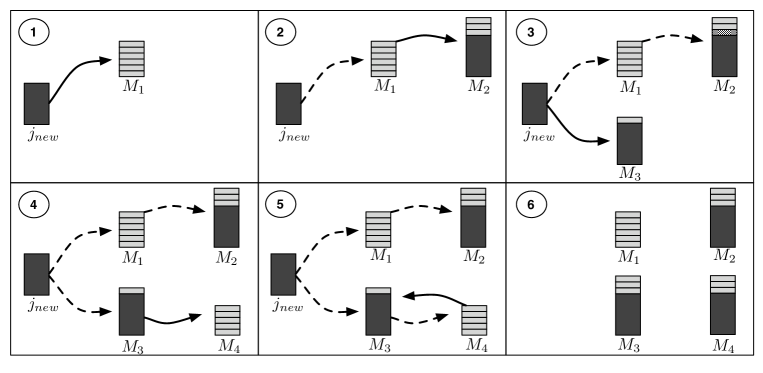
Figure 1: Possible steps when moving jobs to assign a new job $j_{new}$. Big and small jobs depicted in dark and light grey, respectively.

Valid schedule and move.

As alluded to above, the algorithm always maintains a valid partial schedule by moving already assigned jobs. Let us formally define these concepts.

Definition 3.2

A partial schedule is an assignment $\sigma:\mathcal{J}\mapsto\mathcal{M}\cup\{TBD\}$ with the meaning that a job $j$ with $\sigma(j)=TBD$ is not assigned. A partial schedule is valid if each machine $i\in\mathcal{M}$ is assigned at most one big job and $p(\sigma^{-1}(i))\leq 1+R$.

That $i$ is assigned at most one big job is implied here by $p(\sigma^{-1}(i))\leq 1+R$ but will be used for the general case in Section 4. Note also that with this notation a normal schedule is just a partial schedule $\sigma$ with $\sigma^{-1}(TBD)=\emptyset$.

Definition 3.3

A move is a tuple $(j,i)$ of a job $j\in\mathcal{J}$ and a machine $i\in\Gamma_{\sigma}(j)$, where $\Gamma_{\sigma}(j)=\Gamma(j)\setminus\{\sigma(j)\}$ denotes the machines to which $j$ can be assigned apart from $\sigma(j)$.

The main steps of the algorithm are the following. At the start it will try to choose a valid assignment of $j_{new}$ to a machine, i.e., that can be made without violating the target makespan. If no such assignment exists then the algorithm adds the set of jobs that blocked the assignment of $j_{new}$ to the set of jobs we wish to move. It then repeatedly chooses a move of a job $j$ from the set of jobs that is blocking the assignment of $j_{new}$. If the move of $j$ is valid then this will intuitively make more space for $j_{new}$. Otherwise the set of jobs blocking the move of $j$ is added to the list of jobs we wish to move and the procedure will in the next iteration continue to move jobs recursively.

To ensure that we will be able to eventually assign a new job $j_{new}$ it is important which moves we choose. The algorithm will choose between certain moves that we call potential moves, defined so as to guarantee (i) that the procedure terminates and that (ii) if no potential move exists then we shall be able to prove that the dual of [C-LP] is unbounded, contradicting the feasibility of the primal. For this reason, we need to remember to which machines we have already tried to move jobs and which jobs we wish to move. We next describe how the algorithm keeps track of its history and how this affects which move we choose. We then describe the types of potential moves that the algorithm will choose between.

Tree of blockers.

To remember its history, Algorithm 1 has a dynamic tree $\mathcal{T}$ of so-called blockers that “block” moves we wish to do. Blockers of $\mathcal{T}$ have both tree and linear structure. The linear structure is simply the order in time the blockers were added to $\mathcal{T}$. To distinguish between the two we will use child and parent to refer to the tree structure; and after and before to refer to the linear structure. We also use the convention that the blockers $B_{0},B_{1},\dots,B_{t}$ of $\mathcal{T}$ are indexed according to the linear order.

Definition 3.4

A blocker $B$ is a tuple that contains a subset $\mathcal{J}(B)\subseteq\mathcal{J}$ of jobs and a machine $\mathcal{M}(B)$ that takes value $\bot$ if no machine is assigned to the blocker.

To simplify notation, we refer to the machines and jobs in $\mathcal{T}$ by $\mathcal{M}(\mathcal{T})$ and $\mathcal{J}(\mathcal{T})$, respectively. We will conceptually distinguish between small and big blockers and use $\mathcal{M}_{{S}}(\mathcal{T})$ and $\mathcal{M}_{{B}}(\mathcal{T})$ to refer to the subsets of $\mathcal{M}(\mathcal{T})$ containing the machines in small and big blockers, respectively. To be precise, this convention will add a bit to the description of a blocker so as to keep track of whether a blocker is small or big.

The algorithm starts by initializing the tree $\mathcal{T}$ with a special small blocker $B$ as root. Blocker $B$ is special in the sense that it is the only blocker with no machine assigned, i.e., $\mathcal{M}(B)=\bot$. Its job set $\mathcal{J}(B)$ includes the job $j_{new}$ we wish to assign. The next step of the procedure is to repeatedly try to move jobs, until we can eventually assign $j_{new}$. During its execution, the procedure also updates $\mathcal{T}$ based on which move that is chosen so that

1. $\mathcal{M}_{{S}}(\mathcal{T})$ contains those machines to which the algorithm will not try to move any jobs;

2. $\mathcal{M}_{{B}}(\mathcal{T})$ contains those machines to which the algorithm will not try to move any big jobs;

3. $\mathcal{J}(\mathcal{T})$ contains those jobs that the algorithm wishes to move.

Potential moves.

For a move $(j,i)$ to be useful it should be of some job $j\in\mathcal{J}(\mathcal{T})$ as this set contains those jobs we wish to move to make space for the unassigned job $j_{new}$. In addition, the move $(j,i)$ should have a potential of succeeding and be to a machine $i$ where $j$ is allowed to be moved according to $\mathcal{T}$. We refer to such moves as potential moves and a subset of them as valid moves. The difference is that for a potential move to succeed it might be necessary to recursively move other jobs whereas a valid move can be done immediately. With this intuition, let us now define these concepts formally.

Definition 3.5

A move $(j,i)$ of a job $j\in\mathcal{J}(\mathcal{T})$ is a potential

small move:

if $j$ is small and $i\not\in\mathcal{M}_{{S}}(\mathcal{T})$;

big-to-small move:

if $j$ is big, $i\not\in\mathcal{M}(\mathcal{T}),p(S_{i})\leq R,$ and no big job is assigned to $i$;

big-to-big move:

if $j$ is big, $i\not\in\mathcal{M}(\mathcal{T}),p(S_{i})\leq R,$ and a big job is assigned to $i$;

where $S_{i}=\{j\in\sigma^{-1}(i):j\mbox{ is small with $\Gamma_{\sigma}(j)\subseteq\mathcal{M}_{{S}}(\mathcal{T})$}\}$. A potential move $(j,i)$ is valid if the update $\sigma(j)\leftarrow i$ results in a valid schedule.

Note that $S_{i}$ refers to those small jobs assigned to $i$ with no potential moves with respect to the current tree. The condition $p(S_{i})\leq R$ for big moves enforces that we do not try to move big jobs to machines where the load cannot decrease to at most $R$ without removing a blocker already present in $\mathcal{T}$. The algorithm’s behavior depends on the type of the chosen potential move, say $(j,i)$ of a job $j\in\mathcal{J}(B)$ for some blocker $B$:

• If $(j,i)$ is a valid move then the schedule is updated by $\sigma(j)\leftarrow i$. Moreover, $\mathcal{T}$ is updated by removing $B$ and all blockers added after $B$. This will allow us to prove that the procedure terminates with the intuition being that $B$ blocked some move $(j^{\prime},i^{\prime})$ that is more likely to succeed now after $j$ was reassigned.

• If $(j,i)$ is a potential small or big-to-small move that is not valid then the algorithm adds a small blocker $B_{S}$ as a child to $B$ that consists of the machine $i$ and contains all jobs assigned to $i$ that are not already in $\mathcal{T}$. Note that after this, since $B_{S}$ is a small blocker no other jobs will be tried to be moved to $i$. The intuition of this being that assigning more jobs to $i$ would make it less likely to be able to assign $j$ to $i$ in the future.

• If $(j,i)$ is a potential big-to-big move then the algorithm adds a big blocker $B_{B}$ as child to $B$ that consists of the machine $i$ and the big job that is assigned to $i$. Since $B_{B}$ is a big blocker this prevents us from trying to assign more big jobs to $i$ but at the same time allow us to try to assign small jobs. The intuition being that this will not prevent us from assigning $j$ to $i$ if the big job currently assigned to $i$ is reassigned.

We remark that the rules on how to update $\mathcal{T}$ are so that a job can be in at most one blocker whereas a machine can be in at most two blockers (this happens if it is first added in a big blocker and then in a small blocker).

Returning to the example in Figure 1, we can see that after Step $4$, $\mathcal{T}$ consists of the special root blocker with two children, which in turn have a child each. Machines $M_{1},M_{2}$ and $M_{4}$ belong to small blockers whereas $M_{3}$ belongs to a big blocker. Moreover, the moves chosen in the first, second, and the third step are big-to-small, small, and big-to-big, respectively, and from Step $5$ to $6$ a sequence of valid moves is chosen.

Values of moves.

In a specific iteration there might be several potential moves available. For the analysis it is important that they are chosen in a specific order. Therefore, we assign a vector in $\mathbb{R}^{2}$ to each move and Algorithm 1 will then choose the move with minimum lexicographic value.

Definition 3.6

If we let $L_{i}=\sigma^{-1}(i)$ then a potential move $(j,i)$ has value

$$\textnormal{Val}(j,i)=\left\{\begin{array}[]{ll}(0,0)&\mbox{if valid,}\\ (1,p(L_{i}))&\mbox{if small move,}\\ (2,p(L_{i}))&\mbox{if big-to-small,}\\ (3,0)&\mbox{if big-to-big,}\end{array}\right.$$

Note that as the algorithm chooses moves of minimum lexicographic value, it always chooses a valid move if available and a potential small move before a potential move of a big job.

The algorithm.

Algorithm 1 summarizes the algorithm discussed above in a concise definition. Given a valid partial schedule $\sigma$ and an unscheduled job $j_{new}$, we prove that the algorithm preserves a valid schedule by moving jobs until it can assign $j_{new}$. Repeating the procedure by choosing a unassigned job in each iteration until all jobs are assigned then yields Theorem 3.1.

Algorithm 1 SimpleExtendSchedule($\sigma,j_{new}$)

1:  Initialize $\mathcal{T}$ with the root $\mathcal{J}(B)=\{j_{new}\}$ and $\mathcal{M}(B)=\bot$ 

2:  while $\sigma(j_{new})$ is TBD do

3:     Choose a potential move $(j,i)$ with $j\in\mathcal{J}(\mathcal{T})$ of minimum lexicographic value 

4:     Let $B$ be the blocker in $\mathcal{T}$ such that $j\in\mathcal{J}(B)$ 

5:     if $(j,i)$ is valid then

6:        Update the schedule by $\sigma(j)\leftarrow i$ 

7:        Update $\mathcal{T}$ by removing $B$ and all blockers added after $B$ 

8:     else if $(j,i)$ is either a potential small move or a potential big-to-small move then

9:        Add a small blocker $B_{S}$ as child to $B$ with $\mathcal{M}(B_{S})=i$ and $\mathcal{J}(B_{S})=\sigma^{-1}(i)\setminus\mathcal{J}(\mathcal{T})$ 

10:     else {$(j,i)$ is a big-to-big move}

11:        Let $j_{B}$ be the big job such that $\sigma(j_{B})=i$ 

12:        Add a big blocker $B_{B}$ as a child to $B$ with $\mathcal{J}(B_{B})=\{j_{B}\}$ and $\mathcal{M}(B_{B})=i$ 

13:     end if

14:  end while

15:  return  $\sigma$ 

3.1 Analysis

Since the algorithm only updates $\sigma$ if a valid move was chosen we have that the schedule stays valid throughout the execution. It remains to verify that the algorithm terminates and that there always is a potential move to choose.

Before proceeding with the proofs, we need to introduce some notation. When arguing about $\mathcal{T}$ we will let

• $\mathcal{T}_{t}$ be the subtree of $\mathcal{T}$ induced by the blockers $B_{0},B_{1},\dots,B_{t}$;

• $S(\mathcal{T}_{t})=\{j\in\mathcal{J}:\mbox{$j$ is small with $\Gamma_{\sigma}(j)\subseteq\mathcal{M}_{{S}}(\mathcal{T}_{t})$}\}$ and often refer to $S(\mathcal{T})$ by simply $S$; and

• $S_{i}(\mathcal{T}_{t})=\sigma^{-1}(i)\cap S(\mathcal{T}_{t})$ (often refer to $S_{i}(\mathcal{T})$ by $S_{i}$).

The set $S(\mathcal{T}_{t})$ contains the set of small jobs with no potential moves with respect to $\mathcal{T}_{t}$. Therefore no job in $S(\mathcal{T}_{t})$ has been reassigned since $\mathcal{T}_{t}$ became a subtree of $\mathcal{T}$, i.e., since $B_{t}$ was added. We can thus omit the dependence on $\sigma$ when referring to $S(\mathcal{T}_{t})$ and $S_{i}(\mathcal{T}_{t})$ without ambiguity. A related observation that will be useful throughout the analysis is the following. No job in a blocker $B$ of $\mathcal{T}$ has been reassigned after $B$ was added since that would have caused the algorithm to remove $B$ (and all blockers added after $B$).

We now continue by first proving that there always is a potential move to choose if [C-LP] is feasible followed by the proof that the procedure terminates in Section 3.1.2.

3.1.1 Existence of potential moves

We prove that the algorithm never gets stuck if the [C-LP] is feasible.

Lemma 3.7

If [C-LP] is feasible then Algorithm 1 can always choose a potential move.

• Suppose that the algorithm has reached an iteration where no potential move is available. We will show that this implies that the dual of [C-LP] is unbounded and we can thus deduce as required that the primal is infeasible in the case of no potential moves.

  As each solution $(y,z)$ of the dual can be scaled by a scalar $\alpha$ to obtain a new solution $(\alpha y,\alpha z)$, any solution such that $\sum_{i\in\mathcal{M}}y_{i}<\sum_{j\in\mathcal{J}}z_{j}$ implies unboundedness. We proceed by defining such a solution $(y^{*},z^{*})$:

  $$z_{j}^{*}=\begin{cases}2/3&\mbox{if $j\in\mathcal{J}(\mathcal{T})$ is big,}\\ p_{j}=\epsilon&\mbox{if $j\in\mathcal{J}(\mathcal{T})\cup S$ is small,}\\ 0&\mbox{otherwise,}\end{cases}$$

  and

  $$y^{*}_{i}=\begin{cases}1&\mbox{if }i\in\mathcal{M}_{{S}}(\mathcal{T}),\\ \sum_{j\in\sigma^{-1}(i)}z_{j}^{*}&\mbox{otherwise.}\par\end{cases}$$

  Let us first verify that $(y^{*},z^{*})$ is indeed a feasible solution.

  Claim 3.8

  Assuming no potential moves are available, $(y^{*},z^{*})$ is a feasible solution.

  • We need to verify that $y_{i}^{*}\geq\sum_{j\in C}z_{j}^{*}$ for each $i\in\mathcal{M}$ and each $C\in\mathcal{C}(i)$. Recall that the total processing time of the jobs in a configuration is at most $1$. Also observe that $z_{j}^{*}=0$ for jobs not in $\mathcal{J}(\mathcal{T})\cup S$ and we can thus omit such jobs when verifying the constraints.

    Since $z_{j}^{*}\leq p_{j}$ for all $j\in\mathcal{J}$, we have that no constraint involving the variable $y_{i}^{*}$ for $i\in\mathcal{M}_{{S}}(\mathcal{T})$ is violated. Indeed for such a machine $i$ we have $y_{i}^{*}=1$ and $\sum_{j\in\mathcal{C}(i)}z_{j}^{*}\leq\sum_{j\in\mathcal{C}(i)}p_{j}\leq 1$ for any $C\in\mathcal{C}(i)$.

    As a small job $j\in\mathcal{J}(\mathcal{T})$ with a move $(j,i)$ is a potential move if $i\not\in\mathcal{M}_{{S}}(\mathcal{T})$ and no such moves exist by assumption, no small jobs in $\mathcal{J}(\mathcal{T})$ can be moved to machines in $\mathcal{M}\setminus\mathcal{M}_{{S}}(\mathcal{T})$. Also, by definition, no small jobs in $S$ can be moved to a machine $i\not\in\mathcal{M}_{{S}}$. This together with the fact that a big job $j_{B}$ has processing time $1$ and is thus alone in a configuration gives us that a constraint involving $y_{i}^{*}$ for $i\not\in\mathcal{M}_{{S}}(\mathcal{T})$ can only be violated if $y_{i}^{*}<z_{j_{B}}^{*}=2/3$.

    As a machine $i\in\mathcal{M}_{{B}}(\mathcal{T})$ has a big job assigned, we have that for those $y_{i}^{*}\geq 2/3$. Now consider the final case when $i\not\in\mathcal{M}(\mathcal{T})$. If a big job in $\mathcal{J}(\mathcal{T})$ has a move to $i$ then since it is not a potential move $p(S_{i})>R\geq 2/3$. As $z^{*}_{j}=p_{j}=\epsilon$ for small jobs, we have then $y_{i}^{*}=\sum_{j\in\sigma^{-1}(i)}z_{j}^{*}\geq p(S_{i})\geq 2/3$, as required.

    We can thus conclude that no constraint is violated and $(y^{*},z^{*})$ is a feasible solution. $\square$

  Having proved that $(y^{*},z^{*})$ is a feasible solution, the proof of Lemma 3.7 is now completed by showing that the value of the solution is negative.

  Claim 3.9

  We have that $\sum_{i\in\mathcal{M}}y^{*}_{i}<\sum_{j\in\mathcal{J}}z^{*}_{j}$.

  • By the definition of $y^{*}$,

    $$\sum_{i\in\mathcal{M}}y^{*}_{i}=\sum_{i\in\mathcal{M}_{{S}}(\mathcal{T})}1+\sum_{i\not\in\mathcal{M}_{{S}}(\mathcal{T})}\sum_{j\in\sigma^{-1}(i)}z_{j}^{*}$$ (1)

    We proceed by bounding $\sum_{i\in\mathcal{M}_{{S}}(\mathcal{T})}1$ from above by

    $$\sum_{i\in\mathcal{M}_{{S}}(\mathcal{T})}\sum_{j\in\sigma^{-1}(i)}z_{j}^{*}.$$

    Let $B_{0},B_{1},\dots,B_{\ell}$ be the blockers of $\mathcal{T}$ and consider a small blocker $B_{t}$ for some $t=1,\dots,\ell$. By the definition of Algorithm 1, $B_{t}$ was added in an iteration when either a potential small or big-to-small move $(j_{0},i_{t})$ was chosen with $\mathcal{M}(B_{t})=i_{t}$. Suppose first that $(j_{0},i_{t})$ was a potential small move. Then as it was not valid, $p(j_{0})+p(\sigma^{-1}(i_{t}))>1+R.$ This inequality together with the fact that $i_{t}$ is assigned at most one big job $j_{B}$ gives us that if $(j_{0},i_{t})$ is a small move then

    $$\sum_{j\in\sigma^{-1}(i_{t})}z_{j}^{*}=p(\sigma^{-1}(i_{t}))-\left(p(j_{B})-z_{j_{B}}^{*}\right)\geq 1+R-p(j_{0})-\frac{1}{3}=\frac{4}{3}.$$ (2)

    On the other hand, if $(j_{0},i_{t})$ is a potential big-to-small move then as it was not valid

    $$\frac{2}{3}<R<p(\sigma^{-1}(i_{t}))=\sum_{j\in\sigma^{-1}(i_{t})}z_{j}^{*},$$ (3)

    where the equality follows from that $i_{t}$ is only assigned small jobs (since we assumed $(j_{0},i_{t})$ was a big-to-small move).

    From (2) and (3) we can see that $\sum_{i\in\mathcal{M}_{{S}}(\mathcal{T})}1$ is bounded from above by $\sum_{i\in\mathcal{M}_{{S}}(\mathcal{T})}\sum_{j\in\sigma^{-1}(i)}z_{j}^{*}$ if the number of small blockers added because of small moves is greater than the number of small blockers added because of big-to-small moves.

    We proceed by proving this by showing that if $B_{t}$ is a small blocker added because of a potential big-to-small move then $B_{t+1}$ must be a small blocker added because of a small move. Indeed, the definition of a potential big-to-small move $(j_{0},i_{t})$ and the fact that it was not valid imply that

    $$p\left(S_{i_{t}}(\mathcal{T}_{t})\right)\leq R\qquad\mbox{and}\qquad p\left(\sigma^{-1}(i_{t})\right)>R.$$

    As there are no big jobs assigned to $i_{t}$ (using that $(j_{0},i_{t})$ was a big-to-small move), the above inequalities give us that there is always a potential small move of a small job assigned to $i_{t}$ with respect to $\mathcal{T}_{t}$. In other words, we have that $B_{t}$ was not the last blocker added to $\mathcal{T}$ and as small potential moves have the smallest lexicographic value (apart from valid moves), $B_{t+1}$ must be a small blocker added because of a small move. We can thus “amortize” the load of $B_{t+1}$ to increase the load of $B_{t}$. Indeed, if we let $\mathcal{M}(B_{t+1})=i_{t+1}$ then (2) and (3) yield $\sum_{j\in\sigma^{-1}(i_{t})}z_{j}^{*}+\sum_{j\in\sigma^{-1}(i_{t+1})}z_{j}^{*}\geq 2.$

    Pairing each small blocker $B_{t}$ added because of a big-to-small moves with the small blocker $B_{t+1}$ added because of a small move as above allows us to deduce that $|\mathcal{M}_{{S}}(\mathcal{T})|\leq\sum_{i\in\mathcal{M}_{{S}}(\mathcal{T})}\sum_{j\in\sigma^{-1}(i)}z_{j}^{*}$. Combining this inequality with (1) yields

    $$\sum_{i\in\mathcal{M}}y^{*}_{i}\leq\sum_{i\in\mathcal{M}}\sum_{j\in\sigma^{-1}(i)}z_{j}^{*}=\sum_{j\in\mathcal{J}}z_{j}^{*}-z_{j_{new}}^{*}<\sum_{j\in\mathcal{J}}z_{j}^{*},$$

    as required. $\square$

  We have proved that there is a solution $(y^{*},z^{*})$ to the dual that is feasible (Claim 3.8) and has negative value (Claim 3.9) assuming there are no potential moves. In other words, the [C-LP] cannot be feasible if no potential moves can be chosen which completes the proof of the lemma.

  $\square$

3.1.2 Termination

We continue by proving that Algorithm 1 terminates. As the algorithm only terminates when a new job is assigned, Theorem 3.1 follows from Lemma 3.10 together with Lemma 3.7 since then we can, as already explained, repeat the procedure until all jobs are assigned.

The intuition that the procedure terminates, assuming there always is a potential move, is the following. As every time the algorithm chooses a potential move that is not valid a new blocker is added to the tree and as each machine can be in at most 2$|\mathcal{M}|$ blockers, we have that the algorithm must choose a valid move after at most $2|\mathcal{M}|$ steps. Such a move will perhaps trigger more valid moves and each valid move makes a potential move previously blocked more “likely”. We can now guarantee progress by measuring the “likeliness” in terms of the lexicographic value of the move.

Lemma 3.10

Assuming there is always a potential move to choose, Algorithm 1 terminates.

• To prove that the procedure terminates we associate a vector, for each iteration, with the dynamic tree $\mathcal{T}$. We will then show that the lexicographic order of these vectors decreases.

  The vector associated to $\mathcal{T}$ is defined as follows. Let $B_{0},B_{1},\dots,B_{\ell}$ be the blockers of $\mathcal{T}$. With blocker $B_{i}$ we will associate the value vector, denoted by $\textnormal{Val}(B_{i})$, of the move that was chosen in the iteration when $B_{i}$ was added. The vector associated with $\mathcal{T}$ is then simply

  $$(\textnormal{Val}(B_{0}),\textnormal{Val}(B_{1}),\dots,\textnormal{Val}(B_{\ell}),\infty).$$

  If the algorithm adds a new blocker then the lexicographic order clearly decreases as the vector ends with $\infty$. It remains to verify what happens when blockers are removed from $\mathcal{T}$. In that case let the algorithm run until it chooses a potential move that is not valid or terminates. As blockers will be removed in each iteration until it either terminates or chooses a potential move that is not valid we will eventually reach one of these cases. If the algorithm terminates we are obviously done.

  Instead, suppose that starting with $\sigma$ and $\mathcal{T}$ the algorithm does a sequence of steps where blockers are removed until we are left with an updated schedule $\sigma_{k}$, a tree of blockers $\mathcal{T}_{k}$ with $k+1<\ell$ blockers, and a potential move $(j^{\prime},i^{\prime})$ that is not valid is chosen. As a blocker $B$ is removed if a blocker added earlier is removed, we have that $\mathcal{T}_{k}$ equals the subtree of $\mathcal{T}$ induced by $B_{0},B_{1},\dots,B_{k}$.

  We will thus concentrate on comparing the lexicographic value of $(j^{\prime},i^{\prime})$ with that of $B_{k+1}$. Recall that $\textnormal{Val}(B_{k+1})$ equals the value of the move that was chosen when $B_{k+1}$ was added, say $(j_{t},i_{k+1})$ for $j_{t}\in\mathcal{J}(B_{t})$ with $1\leq t\leq k$ and $\mathcal{M}(B_{k+1})=i_{k+1}$.

  A key observation is that since blocker $B_{k+1}$ was removed but not $B_{k}$, the most recent move was of a job $j_{k+1}\in\mathcal{J}(B_{k+1})$ and we have $\sigma(j_{k+1})=i_{k+1}$ and $\sigma_{k}(j_{k+1})\neq i_{k+1}$. Moreover, as $(j_{t},i_{k+1})$ was a potential move when $B_{k+1}$ was added, it is a potential move with respect to $\mathcal{T}_{k}$ (using that $S_{i_{k+1}}\left(\mathcal{T}_{k}\right)$ has not changed). Using these observations we now show that the lexicographic value of $(j_{t},i_{k+1})$ has decreased. As the algorithm always chooses the move of minimum lexicographic value, this will imply $\textnormal{Val}(j^{\prime},i^{\prime})<\textnormal{Val}(B_{k+1})$ as required.

  If $(j_{t},i_{k+1})$ was a small or big-to-small move then $B_{k+1}$ was a small blocker. As no jobs were moved to $i_{k+1}$ after $B_{k+1}$ was added, $p(\sigma_{k}^{-1}(i_{k+1}))<p(\sigma^{-1}(i_{k+1}))$ and we have that the lexicographic value of $(j_{t},i_{k+1})$ has decreased.

  Otherwise if $(j_{t},i_{k+1})$ was a big-to-big move then $j_{k+1}$ must be a big job. As we only have jobs of two sizes, the move of the big job $j_{k+1}$ implies that $(j_{t},i_{k+1})$ now is a valid move which contradicts the assumption that the algorithm has chosen a potential but not valid move $(j^{\prime},i^{\prime})$.

We have thus proved that the vector associated to $\mathcal{T}$ always decreases. As there are at most $2|\mathcal{M}|$ blockers in $\mathcal{T}$ (one small and one big blocker for each machine) and a vector associated to a blocker can take a finite set of values, we conclude that the algorithm terminates. $\square$

4 Proof of Main Result

In this section we extend the techniques presented in Section 3 to prove our main result, i.e., that there is a polynomial time algorithm that estimates the optimal makespan of the restricted assignment problem within a factor of $\frac{33}{17}+\epsilon\approx 1.9412+\epsilon$, where $\epsilon>0$ is an arbitrarily small constant. More specifically, we shall show the following theorem which clearly implies Theorem 1.1. The small loss of $\epsilon$ is as mentioned because the known polynomial time algorithms only solve [C-LP] up to any desired accuracy.

Theorem 4.1

The [C-LP] has integrality gap at most $\frac{33}{17}$.

Throughout this section we let $R=\frac{16}{17}$. The proof follows closely the proof of Theorem 3.1, i.e., we design a local search algorithm that returns a solution with makespan at most $1+R$, assuming the [C-LP] is feasible. The strategy is again to repeatedly call a procedure, now summarized in Algorithm 2, that extends a given partial schedule by assigning a new job while maintaining a valid schedule. Recall that a partial schedule is valid if each machine $i\in\mathcal{M}$ is assigned at most one big job and $p(\sigma^{-1}(i))\leq 1+R$, where now $R=\frac{16}{17}$. We note that a machine is only assigned at most one big job will be a restriction here.

Since we allow jobs of any sizes we need to define what big and small jobs are. In addition, we have medium jobs and partition the big jobs into large and huge jobs.

Definition 4.2

A job $j$ is called big if $p_{j}\geq{11}/{17}$, medium if $11/17>p_{j}>9/17$, and small if $p_{j}\leq 9/17$. Let the sets $\mathcal{J}_{B},\mathcal{J}_{M},\mathcal{J}_{S}$ contain the big, medium, and small jobs, respectively. We will also call a big job $j$ huge if $p_{j}\geq 14/17$ and otherwise large.

The job sizes are chosen so as to optimize the achieved approximation ratio with respect to the analysis and were obtained by solving a linear program.

We shall also need to extend and change some of the concepts used in Section 3. The final goal is still that the procedure shall choose potential moves so as to guarantee (i) that the procedure terminates and that (ii) if no potential move exists then we shall be able to prove that the dual of [C-LP] is unbounded.

The main difficulty compared to the case in Section 3 of two job sizes is the following. A key step of the analysis in the case with only small and big jobs was that if small jobs blocked the move of a big job then we guaranteed that one of the small jobs on the blocking machine had a potential small move. This was to allow us to amortize the load when analyzing the dual. In the general case, this might not be possible when a medium job is blocking the move of a huge job. Therefore, we need to introduce a new conceptual type of blockers called medium blockers that will play a similar role as big blockers but instead of containing a single big job they contain at least one medium job that blocks the move of a huge job. Rather unintuitively, we allow for technical reasons large but not medium or huge jobs to be moved to machines in medium blockers.

Let us now point out the modifications needed starting with the tree $\mathcal{T}$ of blockers.

Tree of blockers.

Similar to Section 3, Algorithm 2 remembers its history by using the dynamic tree $\mathcal{T}$ of blockers. As already mentioned, it will now also have medium blockers that play a similar role as big blockers but instead of containing a single big job they contain a set of medium jobs. We use $\mathcal{M}_{M}(\mathcal{T})$ to refer to the subset of $\mathcal{M}(\mathcal{T})$ containing the machines in medium blockers.

As in the case of two job sizes, Algorithm 2 initializes tree $\mathcal{T}$ with the special small blocker as root that consists of the job $j_{new}$. The next step of the procedure is to repeatedly choose valid and potential moves until we can eventually assign $j_{new}$. During its execution, the procedure now updates $\mathcal{T}$ based on which move that is chosen so that

1. $\mathcal{M}_{{S}}(\mathcal{T})$ contains those machines to which the algorithm will not try to move any jobs;

2. $\mathcal{M}_{{B}}(\mathcal{T})$ contains those machines to which the algorithm will not try to move any huge, large, or medium jobs;

3. $\mathcal{M}_{M}(\mathcal{T})$ contains those machines to which the algorithm will not try to move any huge or medium jobs;

4. $\mathcal{J}(\mathcal{T})$ contains those jobs that the algorithm wishes to move.

We can see that small jobs are treated as in Section 3, i.e., they can be moved to all machines apart from those in $\mathcal{M}_{{S}}(\mathcal{T})$. Similar to big jobs in that section, huge and medium jobs can only be moved to a machine not in $\mathcal{M}(\mathcal{T})$. The difference lies in how large jobs are treated: they are allowed to be moved to machines not in $\mathcal{M}(\mathcal{T})$ but also to those machines only in $\mathcal{M}_{M}(\mathcal{T})$.

Potential moves.

As before a potential move $(j,i)$ will be called valid if the update $\sigma(j)\leftarrow i$ results in a valid schedule, but the definition of potential moves needs to be extended to include the different job sizes. The definition for small jobs remains unchanged: a move $(j,i)$ of a small job $j\in\mathcal{J}(\mathcal{T})$ is a potential small move if $i\not\in\mathcal{M}_{{S}}(\mathcal{T})$. A subset of the potential moves of medium and large jobs will also be called potential small moves.

Definition 4.3

A move $(j,i)$ of a medium or large job $j\in\mathcal{J}(\mathcal{T})$ satisfying $i\not\in\mathcal{M}(\mathcal{T})$ if $j$ is medium and $i\not\in\mathcal{M}_{{B}}(\mathcal{T})\cup\mathcal{M}_{{S}}(\mathcal{T})$ if $j$ is large is a potential

small move:

if $i$ is not assigned a big job.

medium/large-to-big:

if $i$ is assigned a big job.

Note that the definition takes into account the convention that large jobs are allowed to be assigned to machines not in $\mathcal{M}_{{B}}(\mathcal{T})\cup\mathcal{M}_{{S}}(\mathcal{T})$ whereas medium jobs are only allowed to be assigned to machines not in $\mathcal{M}(\mathcal{T})$. The reason for distinguishing between whether $i$ is assigned a big (huge or large) job will become apparent in the analysis. The idea is that if a machine $i$ is not assigned a big job then if it blocks a move of a medium or large job then the dual variables $z^{*}$ will satisfy $\sum_{j\in\sigma^{-1}(i)}z_{j}^{*}\geq 1$, which we cannot guarantee if $i$ is assigned a big job since when setting the dual variables we will round down the sizes of big jobs which might decrease the sum by as much as $6/17$.

It remains to define the potential moves of huge jobs.

Definition 4.4

A move $(j,i)$ of a huge job $j\in\mathcal{J}(\mathcal{T})$ to a machine $i\not\in\mathcal{M}(\mathcal{T})$ is a potential

huge-to-small move:

if no big job is assigned to $i$ and $p(j)+p(S_{i}\cup M_{i})\leq 1+R$;

huge-to-big move:

if a big job is assigned to $i$ and $p(j)+p(S_{i}\cup M_{i})\leq 1+R$;

huge-to-medium move:

if $p(j)+p(S_{i})\leq 1+R$ and $p(j)+p(S_{i}\cup M_{i})>1+R$;

where $S_{i}=\{j\in\sigma^{-1}(i):j\mbox{ is small with }\Gamma_{\sigma}(j)\subseteq\mathcal{M}_{{S}}(\mathcal{T})\}$ and $M_{i}=\mathcal{J}_{M}\cap\sigma^{-1}(i)$.

Again $S_{i}$ denotes the set of small jobs assigned to $i$ with no potential moves with respect to the current tree. The set $M_{i}$ contains the medium jobs currently assigned to $i$. Moves huge-to-small and huge-to-big correspond to the moves big-to-small and big-to-big in Section 3, respectively. The constraint $p(j)+p(S_{i}\cup M_{i})\leq 1+R$ says that such a move should only be chosen if it can become valid by not moving any medium jobs assigned to $i$. The additional move called huge-to-medium covers the case when moving the medium jobs assigned to $i$ is necessary for the move to become valid.

Similar to before, the behavior of the algorithm depends on the type of the chosen potential move. The treatment compared to that in Section 3 of valid moves and potential small moves is unchanged; the huge-to-small move is treated as the big-to-small move; and the medium/large-to-big and huge-to-big moves are both treated as the big-to-big move were in Section 3. It remains to specify what Algorithm 2 does in the case when a potential huge-to-medium move (that is not valid) is chosen, say $(j,i)$ of a job $j\in\mathcal{J}(B)$ for some blocker $B$. In that case the algorithm adds a medium blocker $B_{M}$ as child to $B$ that consists of the machine $i$ and the medium jobs assigned to $i$. This prevents other huge or medium jobs to be assigned to $i$. Also note that constraints $p(j)+p(S_{i})\leq 1+R$ and $p(j)+p(S_{i}\cup M_{i})>1+R$ imply that there is at least one medium job assigned to $i$.

We remark that the rules on how to update $\mathcal{T}$ is again so that a job can be in at most one blocker whereas a machine can now be in at most three blockers (this can happen if it is first added in a medium blocker, then in a big blocker, and finally in a small blocker).

Values of moves.

As in Section 3, it is important in which order the moves are chosen, Therefore, we assign a value vector to each potential move and Algorithm 2 chooses then, in each iteration, the move with smallest lexicographic value.

Definition 4.5

If we let $L_{i}=\sigma^{-1}(i)$ then a potential move $(j,i)$ has value

$$\textnormal{Val}(j,i)=\left\{\begin{array}[]{ll}(0,0)&\mbox{ if valid,}\\ (p(j),p(L_{i}))&\mbox{ if small move,}\\ (2,0)&\mbox{ if medium/large-to-big,}\\ (3,p(L_{i}))&\mbox{ if huge-to-small,}\\ (4,0)&\mbox{ if huge-to-big,}\\ (5,|L_{i}\cap\mathcal{J}_{M}|)&\mbox{ if huge-to-medium.}\end{array}\right.$$

Note that as before, the algorithm chooses a valid move if available and a potential small move before any other potential move. Moreover, it chooses the potential small move of the smallest job available.

The algorithm.

Algorithm 2 summarizes the algorithm concisely using the concepts described previously. Given a valid partial schedule $\sigma$ and an unscheduled job $j_{new}$, we shall prove that it preserves a valid schedule by moving jobs until it can assign $j_{new}$. Repeating the procedure until all jobs are assigned then yields Theorem 4.1.

Algorithm 2 ExtendSchedule($\sigma,j_{new}$):

1:  Initialize $\mathcal{T}$ with the root $\mathcal{J}(B)=\{j_{new}\}$ and $\mathcal{M}(B)=\bot$ 

2:  while $\sigma(j_{new})$ is TBD do

3:     Choose a potential move $(j,i)$ with $j\in\mathcal{J}(\mathcal{T})$ of minimum lexicographic value 

4:     Let $B$ be the blocker in $\mathcal{T}$ such that $j\in\mathcal{J}(B)$ 

5:     if $(j,i)$ is valid then

6:        Update the schedule by $\sigma(j)\leftarrow i$ 

7:        Update $\mathcal{T}$ by removing $B$ and all blockers added after $B$ 

8:     else if $(j,i)$ is either a potential small or huge-to-small move then

9:        Add a small blocker $B_{S}$ as child to $B$ with $\mathcal{M}(B_{S})=i$ and $\mathcal{J}(B_{S})=\sigma^{-1}(i)\setminus\mathcal{J}(\mathcal{T})$;

10:     else if $(j,i)$ is either a potential large/medium-to-big or huge-to-big move then

11:        Let $j_{B}$ be the big job such that $\sigma(j_{B})=i$ 

12:        Add a big blocker $B_{B}$ as a child to $B$ in $\mathcal{T}$ with $\mathcal{J}(B_{B})=\{j_{B}\}$ and $\mathcal{M}(B_{B})=i$ 

13:     else {$(j,i)$ is a potential huge-to-medium move}

14:        Add a medium blocker $B_{M}$ as child to $B$ with $\mathcal{M}(B_{M})=i$ and $\mathcal{J}(B_{M})=\sigma^{-1}(i)\cap\mathcal{J}_{M}$ 

15:     end if

16:  end while

17:  return  $\sigma$ 

4.1 Analysis

As Algorithm 1 for the case of two job sizes, Algorithm 2 only updates the schedule if a valid move is chosen so it follows that the schedule stays valid throughout the execution. It remains to verify that the algorithm terminates and that the there always is a potential move to choose.

The analysis is similar to that of the simpler case but involves more case distinctions. When arguing about $\mathcal{T}$ we again let

• $\mathcal{T}_{t}$ be the subtree of $\mathcal{T}$ induced by the blockers $B_{0},B_{1},\dots,B_{t}$;

• $S(\mathcal{T}_{t})=\{j\in\mathcal{J}:\mbox{$j$ is small with $\Gamma_{\sigma}(j)\subseteq\mathcal{M}_{{S}}(\mathcal{T}_{t})$}\}$ and often refer to $S(\mathcal{T})$ by simply $S$; and

• $S_{i}(\mathcal{T}_{t})=\sigma^{-1}(i)\cap S(\mathcal{T}_{t})$ (often refer to $S_{i}(\mathcal{T})$ by $S_{i}$).

As in the case of two job sizes, the set $S(\mathcal{T}_{t})$ contains the set of small jobs with no potential moves with respect to $\mathcal{T}_{t}$. Therefore no job in $S(\mathcal{T}_{t})$ has been reassigned since $\mathcal{T}_{t}$ became a subtree of $\mathcal{T}$, i.e., since $B_{t}$ was added. We can thus again omit without ambiguity the dependence on $\sigma$ when referring to $S(\mathcal{T}_{t})$ and $S_{i}(\mathcal{T}_{t})$. The following observation will again be used throughout the analysis. No job in a blocker $B$ of $\mathcal{T}$ has been reassigned after $B$ was added since that would have caused the algorithm to remove $B$ (and all blockers added after $B$).

In Section 4.1.1 we start by presenting the proof that the algorithm always can choose a potential move if [C-LP] is feasible. We then present the proof that the algorithm always terminates in Section 4.1.2. As already noted, by repeatedly calling Algorithm 2 until all jobs are assigned we will, assuming [C-LP] feasible, obtain a schedule of the jobs with makespan at most $1+R$ which completes the proof of Theorem 4.1.

4.1.1 Existence of potential moves

We prove that the algorithm never gets stuck if the [C-LP] is feasible.

Lemma 4.6

If [C-LP] is feasible then Algorithm 2 can always pick a potential move.

• Suppose that the algorithm has reached an iteration where no potential move is available. Similar to the proof of Lemma 3.7 we will show that this implies that the dual is unbounded and hence the primal is not feasible. We will do so by defining a solution $(y^{*},z^{*})$ to the dual with $\sum_{i\in\mathcal{M}}y^{*}_{i}<\sum_{j\in\mathcal{J}}z^{*}_{j}$. Define $z^{*}$ and $y^{*}$ by

  $$z^{*}_{j}=\begin{cases}11/17,&\mbox{if $j\in\mathcal{J}(\mathcal{T})$ is big},\\ 9/17,&\mbox{if $j\in\mathcal{J}(\mathcal{T})$ is medium},\\ p_{j},&\mbox{if $j\in\mathcal{J}(\mathcal{T})\cup S$ is small},\\ 0,&\mbox{otherwise,}\end{cases}$$

  and

  $$y^{*}_{i}=\begin{cases}1&\text{if $i\in\mathcal{M}_{{S}}(\mathcal{T})$},\\ \sum_{j\in\sigma^{-1}(i)}z_{j}^{*}&\text{otherwise.}\end{cases}$$

  A natural interpretation of $z^{*}$ is that we have rounded down processing times where big jobs with processing times in $[11/17,1]$ are rounded down to $11/17$; medium jobs with processing times in $[9/17,11/17]$ are rounded down to $9/17$; and small jobs are left unchanged.

  The proof of the lemma is now completed by showing that $(y^{*},z^{*})$ is a feasible solution (Claim 4.7) and that the objective value is negative (Claim 4.8).

  Claim 4.7

  Assuming no potential moves are available, $(y^{*},z^{*})$ is a feasible solution.

  • We need to verify that $y_{i}^{*}\geq\sum_{j\in C}z_{j}^{*}$ for each $i\in\mathcal{M}$ and each $C\in\mathcal{C}(i)$. Recall that the total processing time of the jobs in a configuration is at most $1$. Also observe as in the simpler case that $z_{j}^{*}=0$ for jobs not in $\mathcal{J}(\mathcal{T})\cup S$ and we can thus omit them when verifying the constraints.

    As in the previous case, no constraint involving the variable $y_{i}^{*}$ for $i\in\mathcal{M}_{{S}}(\mathcal{T})$ is violated. Indeed, for such a machine $i$ we have $y_{i}^{*}=1$ and $\sum_{j\in\mathcal{C}(i)}z_{j}^{*}\leq\sum_{j\in\mathcal{C}(i)}p_{j}\leq 1$ for any configuration $C\in\mathcal{C}(i)$.

  We continue by distinguishing between the remaining cases when $i\not\in\mathcal{M}(\mathcal{T}),i\in\mathcal{M}_{{B}}(\mathcal{T})\setminus\mathcal{M}_{{S}}(\mathcal{T})$, and $i\in\mathcal{M}_{M}(\mathcal{T})\setminus(\mathcal{M}_{{S}}(\mathcal{T})\cup\mathcal{M}_{{B}}(\mathcal{T}))$.

$i\not\in\mathcal{M}(\mathcal{T})$:

A move $(j,i)$ to machine $i\not\in\mathcal{M}(\mathcal{T})$ is a potential move if $j\in\mathcal{J}(\mathcal{T})$ is a small, medium, or large job. By assumption we have thus that no such jobs in $\mathcal{J}(\mathcal{T})$ have any moves to $i$. We also have, by definition, that no job in $S$ has a move to $i\not\in\mathcal{M}_{{S}}(\mathcal{T})$.

Now consider the final case when a huge job $j_{H}\in\mathcal{J}(\mathcal{T})$ has a move $(j_{H},i)$. Then since it is not a potential huge-to-small, huge-to-medium, or huge-to-big move

$$p(j_{H})+p(S_{i})>1+R\qquad\mbox{and hence}\qquad p(S_{i})>R.$$

Since $p(j_{H})\geq{14}/{17}$ but $z_{j_{H}}^{*}=11/17$ a configuration $C\in\mathcal{C}(i)$ with $j_{H}\in C$ satisfy

$$\sum_{j\in C}z_{j}^{*}\leq z_{j_{H}}^{*}+(1-p(j_{H}))\leq\frac{11}{17}+\left(1-\frac{14}{17}\right)=\frac{14}{17},$$ (4)

which is less than $\frac{16}{17}=R<p(S_{i})\leq\sum_{j\in\sigma^{-1}(i)}z_{j}^{*}\leq y^{*}_{i}$ where we used that $S_{i}$ only contains small jobs for the second inequality.

$i\in\mathcal{M}_{{B}}(\mathcal{T})\setminus\mathcal{M}_{{S}}(\mathcal{T})$:

A move to machine $i\not\in\mathcal{M}_{{S}}(\mathcal{T})$ is a potential move if $j\in\mathcal{J}(\mathcal{T})$ is a small job. By the assumption that there are no potential moves and by the definition of $S$, we have thus that there is no small job in $\mathcal{J}(\mathcal{T})\cup S$ with a move to $i$. In other words, all small jobs with $z_{j}^{*}>0$ that can be moved to $i$ are already assigned to $i$. Now let $j_{B}$ be the big job such that $\sigma(j_{B})=i$ which must exist since machine $i$ is contained in a big blocker. As both medium and big (large and huge) jobs have processing time strictly greater than $1/2$, a configuration $C\in\mathcal{C}(i)$ can contain at most one such job $j_{0}$. Since $z_{j_{0}}^{*}\leq 11/17$ and $z_{j_{B}}^{*}=11/17$ we have that a configuration $C\in\mathcal{C}(i)$ with $j_{0}\in C$ cannot violate feasibility. Indeed,

$$\sum_{j\in C}z_{j}^{*}\leq z_{j_{0}}^{*}+\sum_{j\in\sigma^{-1}(i)\setminus j_{B}}z_{j}^{*}\leq z_{j_{B}}^{*}+\sum_{j\in\sigma^{-1}(i)\setminus j_{B}}z_{j}^{*}=y^{*}_{i}.$$ (5)

$i\in\mathcal{M}_{M}(\mathcal{T})\setminus(\mathcal{M}_{{S}}(\mathcal{T})\cup\mathcal{M}_{{B}}(\mathcal{T})):$

By the definition of $S$ and the assumption that there are no potential moves, no small or large jobs in $\mathcal{J}(\mathcal{T})\cup S$ have any moves to $i$. As $i$ is contained in a medium blocker, there is a medium job $j_{M}$ such that $\sigma(j_{M})=i$. As both medium and huge jobs have processing time strictly greater than $1/2$, a configuration $C\in\mathcal{C}(i)$ can contain at most one such job $j_{0}$.

If $j_{0}$ is medium then $z_{j_{0}}^{*}\leq z_{j_{M}}^{*}$ and we have by Inequality (5) (substituting $j_{B}$ with $j_{M}$) that the constraint is not violated. Otherwise if $j_{0}$ is huge then from (4) (substituting $j_{H}$ with $j_{0}$) we have that $\sum_{j\in C}z_{j}^{*}\leq\frac{14}{17}$ for any configuration $C\in\mathcal{C}(i)$ with $j_{0}\in C$.

We shall now show that $y_{i}^{*}\geq\frac{14}{17}$ which completes this case. If $i$ is assigned more than one medium job then $y_{i}^{*}\geq 1$. Instead suppose that the only medium job assigned to $i$ is $j_{M}$. Since the medium blocker $B_{M}$, with $\mathcal{M}(B_{M})=i$ and $\mathcal{J}(B_{M})=\{j_{M}\}$, was added to $\mathcal{T}$ because the algorithm chose a potential huge-to-medium move we have

$$p(S_{i}(\mathcal{T}^{\prime}))+p(j_{M})>R.$$

where $\mathcal{T}^{\prime}$ refer to the tree of blockers at the time when $B_{M}$ was added.

As each blocker in $\mathcal{T}^{\prime}$ is also in $\mathcal{T}$, $p(S_{i})\geq p(S_{i}(\mathcal{T}^{\prime}))$ and the above inequality yields,

$$y_{i}^{*}\geq p(S_{i})+p(j_{M})-(p(j_{M})-z_{j_{M}}^{*})\geq R-\left(\frac{11}{17}-\frac{9}{17}\right)\geq\frac{14}{17},$$

as required.

We have thus verified all the cases which completes the proof of the claim. $\square$

Having verified that $(y^{*},z^{*})$ is a feasible solution, the proof is now completed by showing that the value of the solution is negative.

Claim 4.8

We have that $\sum_{i\in\mathcal{M}}y^{*}_{i}<\sum_{j\in\mathcal{J}}z_{j}^{*}$.

• By the definition of $y^{*}$,

  $$\sum_{i\in\mathcal{M}}y^{*}_{i}=\sum_{i\in\mathcal{M}_{{S}}(\mathcal{T})}1+\sum_{i\not\in\mathcal{M}_{{S}}(\mathcal{T})}\sum_{j\in\sigma^{-1}(i)}z_{j}^{*}.$$ (6)

  Similar to the case with two job sizes in Section 3, we proceed by bounding $\sum_{i\in\mathcal{M}_{{S}}(\mathcal{T})}1$ from above by $\sum_{i\in\mathcal{M}_{{S}}(\mathcal{T})}\sum_{j\in\sigma^{-1}(i)}z_{j}^{*}$. Let $B_{0},B_{1},\dots,B_{\ell}$ be the blockers of $\mathcal{T}$ and consider a small blocker $B_{t}$ for some $t=1,\dots,\ell$ with $\mathcal{M}(B_{t})=i_{t}$.

  By the definition of the procedure, small blocker $B_{t}$ has been added in an iteration when either a potential small or huge-to-small move $(j_{0},i_{t})$ was chosen. Let us distinguish between the three cases when $(j_{0},i_{t})$ was a small move of a small job, $(j_{0},i_{t})$ was a small move of a medium or large job, and $(j_{0},i_{t})$ was a huge-to-small move.

$(j_{0},i_{t})$ was a small move of a small job:

Since the move was not valid,

$$p(j_{0})+p(\sigma^{-1}(i_{t}))>1+R.$$

As a big job with processing time in $[11/17,1]$ is rounded down to $11/17$ and a medium job with processing time in $[9/17,11/17]$ is rounded down to $9/17$, the sum $\sum_{j\in\sigma^{-1}(i_{t})}z_{j}^{*}$ will depend of the number of big and medium jobs assigned to $i_{t}$. Indeed, if we let $L_{i_{t}}=\sigma^{-1}(i_{t})\cap\mathcal{J}_{B}$ and $M_{i_{t}}=\sigma^{-1}(i_{t})\cap\mathcal{J}_{M}$ be the big and medium jobs assigned to $i_{t}$, respectively. Then on the one hand,

$$\sum_{j\in\sigma^{-1}(i_{t})}z_{j}^{*}\geq 1+R-p(j_{0})-\left(1-\frac{11}{17}\right)|L_{i_{t}}|-\left(\frac{11}{17}-\frac{9}{17}\right)|M_{i_{t}}|,$$

which equals

$$\frac{33}{17}-\frac{6}{17}\left(|L_{i_{t}}|+\frac{|M_{i_{t}}|}{3}\right)-p(j_{0}).$$

On the other hand, if (i) $|L_{i_{t}}|\geq 2$, (ii) $|L_{i_{t}}|\geq 1$ and $|M_{i}|\geq 1$ or (iii) $|M_{i_{t}}|\geq 3$ then clearly

$$\sum_{j\in\sigma^{-1}(i_{t})}z_{j}^{*}\geq\frac{11}{17}+\frac{9}{17}\geq\frac{20}{17}.$$

Combining these two bounds we get (since $j_{0}$ is small and thus $p(j_{0})\leq 9/17$) that

$$\sum_{j\in\sigma^{-1}(i_{t})}z_{j}^{*} \geq\min\left[\frac{27}{17}-p(j_{0}),\frac{20}{17}\right]\geq\frac{18}{17} (j_{0},i_{t})$$ if was a small move of a small job. (7)

$(j_{o},i_{t})$ was a small move of a medium or large job:

Since the move was not valid, we have again

$$p(j_{0})+p(\sigma^{-1}(i_{t}))>1+R.$$

By the definition of potential small moves it must be that there is no big job assigned to $i_{t}$. If there are more than one medium job assigned to $i$ then clearly $\sum_{j\in\sigma^{-1}(i_{t})}z_{j}^{*}\geq 1$.

Otherwise, if there is at most one medium job assigned to $i_{t}$ that might have been rounded down from $11/17$ to $9/17$ we use the inequality $p(j_{0})+p(\sigma^{-1}(i_{t}))>1+R$ to derive

$$\sum_{j\in\sigma^{-1}(i_{t})}z_{j}^{*}\geq 1+R-p(j_{0})-\left(\frac{11}{17}-\frac{9}{17}\right)=\frac{31}{17}-p(j_{0})\geq 1,$$

For the final inequality we used that the processing time of medium and large jobs is at most ${14}/{17}$. Summarizing again, we have

$$\sum_{j\in\sigma^{-1}(i_{t})}z_{j}^{*} \geq 1 (j_{0},i_{t})$$ if was a potential small move of a medium or large job. (8)

$(j_{0},i_{t})$ was a huge-to-small move:

Similar to the case of two job sizes in Section 3 where we considered the big-to-small move, we will show that we can amortize the cost from the blocker $B_{t+1}$. Indeed, since the move $(j_{0},i_{t})$ was not valid and by the definition of a potential huge-to-small move we have

$$p(j_{0})+p(\sigma^{-1}(i_{t}))>1+R\qquad\mbox{and}\qquad p(j_{0})+p\left(S_{i_{t}}(\mathcal{T}_{t})\cup M_{i_{t}}\right)\leq 1+R,$$ (9)

where we let $M_{i_{t}}$ contain the medium jobs assigned to $i_{t}$ at the time when $B_{t}$ was added. Recall that $S_{i_{t}}(\mathcal{T}_{t})$ contains those small jobs that have no potential moves with respect to the tree of blockers $\mathcal{T}_{t}$ after $B_{t}$ was added. As $B_{t}$ has not been removed from $\mathcal{T}$ both these sets have not changed. In particular, since $i_{t}$ is not assigned a big job (using the definition of huge-to-small move) we have that there must be a small job $j^{\prime}\in\sigma^{-1}(i_{t})\setminus(S_{i_{t}}(\mathcal{T}_{t})\cup M_{i_{t}})$ that has a potential small $(j^{\prime},i^{\prime})$ move with respect to $\mathcal{T}_{t}$.

The above discussion implies that $t<\ell$. Moreover, the value of $(j^{\prime},i^{\prime})$ equals $(p(j^{\prime}),p(\sigma^{-1}(i^{\prime})))$. As the procedure always chooses a potential move with minimum lexicographic value we have that $B_{t+1}$ is a small blocker added because a potential small move was chosen of a small job with processing time at most $p(j^{\prime})$.

If we let $\mathcal{M}(B_{t+1})=i_{t+1}$ we have thus by (7)

$$\sum_{j\in\sigma^{-1}(i_{t+1})}z_{j}^{*}\geq\min\left[\frac{27}{17}-p(j^{\prime}),\frac{20}{17}\right]\geq\frac{18}{17}.$$ (10)

We proceed by showing that we can use this fact to again amortize the cost as done in the simpler analysis, i.e., that

$$\sum_{j\in\sigma^{-1}(i_{t})}z_{j}^{*}+\sum_{j\in\sigma^{-1}(i_{t+1})}z_{j}^{*}\geq 2.$$ (11)

For this reason, let us distinguish between three subcases depending on the number of medium jobs assigned to $i_{t}$.

$i_{t}$ is assigned at least two medium jobs:

Since medium jobs have value $9/17$ in the dual this clearly implies that $\sum_{j\in\sigma^{-1}(i_{t})}z_{j}^{*}\geq 18/17$ so no amortizing is needed and (11) holds in this case.

$i_{t}$ is assigned one medium job:

Let $j_{M}$ denote the medium job assigned to $i_{t}$. In addition we have that the small job $j^{\prime}$ is assigned to $i_{t}$. We have thus that $\sum_{j\in\sigma^{-1}(i)}z_{j}^{*}\geq 9/17+p(j^{\prime})$. So if $p(j^{\prime})\geq 7/17$ then we can amortize because $\sum_{j\in\sigma^{-1}(i_{t+1})}z_{j}^{*}$ is at least $18/17$.

Now consider the case when $p(j^{\prime})<7/17$. By the assumption that only one medium job is assigned to $i_{t}$ and since $p(j_{0})+p(\sigma^{-1}(i_{t}))\geq 1+R$ we have

$$\sum_{j\in\sigma^{-1}(i_{t})}z_{j}^{*}\geq R-\left(\frac{11}{17}-\frac{9}{17}\right)=\frac{14}{17}.$$

Moreover, as the case when $p(j^{\prime})<7/17$ is considered, we have from (10) that

$$\sum_{j\in\sigma^{-1}(i_{t+1})}z_{j}^{*}\geq\frac{20}{17},$$

which implies that (11) is valid also in this case.

$i_{t}$ is not assigned any medium jobs:

As $i_{t}$ in this case is not assigned any medium or big jobs and the huge-to-small move $(j_{0},i_{t})$ was not valid,

$$\sum_{j\in\sigma^{-1}(i_{t})}z_{j}^{*}>R\geq\frac{16}{17}.$$

That we can amortize now follows from (10) that we always have $\sum_{j\in\sigma^{-1}(i_{t+1})}z_{j}^{*}\geq\frac{18}{17}.$

We have thus shown that a blocker $B_{t}$ added because of a huge-to-small move can be paired with the following blocker $B_{t+1}$ that was added because of a potential small move of a small job. As seen above this give us that we can amortize the cost exactly as done in the simpler case and we deduce that $|\mathcal{M}_{{S}}(\mathcal{T})|\leq\sum_{i\in\mathcal{M}_{{S}}(\mathcal{T})}\sum_{j\in\sigma^{-1}(i)}z_{j}^{*}$. Combining this inequality with (1) yields

$$\sum_{i\in\mathcal{M}}y^{*}_{i}\leq\sum_{i\in\mathcal{M}}\sum_{j\in\sigma^{-1}(i)}z_{j}^{*}=\sum_{j\in\mathcal{J}}z_{j}^{*}-z_{j_{new}}^{*}<\sum_{j\in\mathcal{J}}z_{j}^{*},$$

as required. $\square$

We have proved that there is a solution $(y^{*},z^{*})$ to the dual that is feasible (Claim 4.7) and has negative value (Claim 4.8) assuming there are no potential moves. In other words, the [C-LP] cannot be feasible if no potential moves can be chosen which completes the proof of the lemma. $\square$

4.1.2 Termination

As the algorithm only terminates when a new job is assigned, Theorem 4.1 follows from the lemma below together with Lemma 4.6 since then we can, as already explained, repeat the procedure until all jobs are assigned.

Lemma 4.9

Assuming there is always a potential move to choose, Algorithm 2 terminates.

• As in the proof of Lemma 3.10, we consider the $i$’th iteration of the algorithm and associate the vector

  $$(\textnormal{Val}(B_{1}),\textnormal{Val}(B_{2}),\dots,\textnormal{Val}(B_{\ell}),\infty).$$

  with $\mathcal{T}$ where the blockers are ordered in the order they were added and $\textnormal{Val}(B_{i})$ equals the value of the move chosen when $B_{i}$ was added. We shall now prove that the value of the vector associated with $\mathcal{T}$ decreases no matter the step chosen in the next iteration.

  If a new blocker is added in the $i+1$’th iteration the lexicographic order clearly decreases as the vector ends with $\infty$. It remains to verify what happens when blockers are removed from $\mathcal{T}$. In that case let the algorithm run until it chooses a potential move that is not valid or terminates. As blockers will be removed in each iteration until it either terminates or chooses a potential move that is not valid we will eventually reach one of these cases. If the algorithm terminates we are obviously done.

  Instead, suppose that starting with $\sigma$ and $\mathcal{T}$ the algorithm does a sequence of steps where blockers are removed until we are left with an updated schedule $\sigma_{k}$, a $\mathcal{T}_{k}$ with $k+1<\ell$ blockers, and a potential move $(j^{\prime},i^{\prime})$ that is not valid is chosen. As a blocker $B$ is removed if a blocker added earlier is removed, we have that $\mathcal{T}_{k}$ equals the subtree of $\mathcal{T}$ induced by $B_{0},B_{1},\dots,B_{k}$.

  We will thus concentrate on comparing the lexicographic value of $(j^{\prime},i^{\prime})$ with that of $B_{k+1}$. The value of $B_{k+1}$ equals of the value of the move chosen when $B_{k+1}$ was added, say $(j_{t},i_{k+1})$ for $j_{t}\in\mathcal{J}(B_{t})$ with $1\leq t\leq k$ and $\mathcal{M}(B_{k+1})=i_{k+1}$.

  A key observation is that since blocker $B_{k+1}$ was removed but not $B_{k}$, the most recent move was of a job $j_{k+1}\in\mathcal{J}(B_{k+1})$ and we have $\sigma(j_{k+1})=i_{k+1}$ and $\sigma_{k}(j_{k+1})\neq i_{k+1}$. Moreover, as $(j_{t},i_{k+1})$ was a potential move when $B_{k+1}$ was added, it is a potential move with respect to $\mathcal{T}_{k}$ (using that $S_{i_{k+1}}\left(\mathcal{T}_{k}\right)$ has not changed). Using these observations we now show that the lexicographic value of $(j_{t},i_{k+1})$ has decreased. As the algorithm always picks the move of minimum lexicographic value, this will imply $\textnormal{Val}(j^{\prime},i^{\prime})<\textnormal{Val}(B_{k+1})$ as required.

  If $(j_{t},i_{k+1})$ was a small or huge-to-small move then $B_{k+1}$ was a small blocker. As no jobs were moved to $i_{k+1}$ after $B_{k+1}$ was added, $p(\sigma_{k}^{-1}(i_{k+1}))<p(\sigma^{-1}(i_{k+1})$ and we have that the lexicographic value of $(j_{t},i_{k+1})$ has decreased.

If $(j_{t},i_{k+1})$ was a medium/large-to-big (or huge-to-big move) then $j_{k+1}$ must be a big job and hence the machine $i_{k+1}$ has no longer a big job assigned. This implies that the move $(j_{t},i_{k+1})$ is now a potential small (or huge-to-small using that no medium jobs are moved to machines in big blockers) with smaller lexicographic value.

Finally, if $(j_{t},i_{k+1})$ was a huge-to-medium move then $j_{k+1}$ must be a medium job and since no medium jobs have potential moves to machines in medium blockers we have that $|\sigma_{k}^{-1}(i)\cap\mathcal{J}_{M}|<|\sigma^{-1}(i)\cap\mathcal{J}_{M}|$ which implies that the lexicographic value of $(j_{t},i_{k+1})$ also decreased in this case.

We have thus proved that the vector associated to $\mathcal{T}$ always decreases. As there are at most $3|\mathcal{M}|$ blockers in $\mathcal{T}$ (one small, medium, and big blocker for each machine) and a vector associated to a blocker can take a finite set of values, we conclude that the algorithm eventually terminates. $\square$

5 Conclusions

We have shown that the configuration LP gives a polynomial time computable lower bound on the optimal makespan that is strictly better than two. Our techniques are mainly inspired by recent developments on the related Santa Claus problem and gives a local search algorithm to also find a schedule of the same performance guarantee, but is not known to converge in polynomial time.

Similar to the Santa Claus problem, this raises the open question whether there is an efficient rounding of the configuration LP that matches the bound on the integrality gap (see also [8] for a comprehensive discussion on open problems related to the difference between estimation and approximation algorithms). Another interesting direction is to improve the upper or lower bound on the integrality gap for the restricted assignment problem: we show that it is no worse than $33/17$ and it is only known to be no better than $1.5$ which follows from the NP-hardness result. One possibility would be to find a more elegant generalization of the techniques, presented in Section 3 for two job sizes, to arbitrary processing times (instead of the exhaustive case distinction presented in this paper).

To obtain a tight analysis, it would be natural to start with the special case of graph balancing for which the $1.75$-approximation algorithm by Ebenlendr et al. [6] remains the best known. We remark that the restriction $p_{ij}\in\{p_{j},\infty\}$ is necessary as the integrality gap of the configuration LP for the general case is known to be $2$ even if a job can be assigned to at most $2$ machines [19].

6 Acknowledgements

I am grateful to Johan Håstad for many useful insights and comments. I also wish to thank Tobias Mömke and Lukáš Poláček for useful comments on the exposition. This research is supported by ERC Advanced investigator grant 226203.

References

- [1] A. Asadpour, U. Feige, and A. Saberi. Santa claus meets hypergraph matchings. In Proceedings of the 11th international workshop and 12th international workshop on Approximation, Randomization and Combinatorial Optimization, 2008. See authors’ homepages for the lower bound of instead of the claimed in the conference version.
- [2] A. Asadpour and A. Saberi. An approximation algorithm for max-min fair allocation of indivisible goods. SIAM Journal on Computing, 39(7):2970–2989, 2010.
- [3] N. Bansal and M. Sviridenko. The santa claus problem. In Proceedings of the thirty-eighth annual ACM symposium on Theory of computing (STOC), pages 31–40, 2006.
- [4] M. Bateni, M. Charikar, and V. Guruswami. Maxmin allocation via degree lower-bounded arborescences. In Proceedings of the 41st annual ACM symposium on Theory of computing (STOC), pages 543–552, 2009.
- [5] D. Chakrabarty, J. Chuzhoy, and S. Khanna. On allocating goods to maximize fairness. In Proceedings of the 2009 50th Annual IEEE Symposium on Foundations of Computer Science (FOCS), pages 107–116, 2009.
- [6] T. Ebenlendr, M. Krčál, and J. Sgall. Graph balancing: a special case of scheduling unrelated parallel machines. In Proceedings of the nineteenth annual ACM-SIAM symposium on Discrete algorithms (SODA), pages 483–490, 2008.
- [7] U. Feige. On allocations that maximize fairness. In Proceedings of the Nineteenth Annual ACM-SIAM Symposium on Discrete Algorithms (SODA), pages 287–293, 2008.
- [8] U. Feige. On estimation algorithms vs approximation algorithms. In IARCS Annual Conference on Foundations of Software Technology and Theoretical Computer Science (FSTTCS), pages 357–363, 2008.
- [9] B. Haeupler, B. Saha, and A. Srinivasan. New constructive aspects of the lovasz local lemma. To appear in Proceedings of the 51st Annual IEEE Symposium on Foundations of Computer Science (FOCS), 2010.
- [10] D. S. Hochbaum and D. B. Shmoys. A polynomial approximation scheme for scheduling on uniform processors: Using the dual approximation approach. SIAM Journal on Computing, pages 539–551, 1988.
- [11] E. Horowitz and S. Sahni. Exact and approximate algorithms for scheduling nonidentical processors. Journal of the ACM, 23(2):317–327, 1976.
- [12] K. Jansen and L. Porkolab. Improved approximation schemes for scheduling unrelated parallel machines. Mathematics of Operations Research, 26:324–338, 2001.
- [13] J. K. Lenstra, D. B. Shmoys, and E. Tardos. Approximation algorithms for scheduling unrelated parallel machines. Mathematical Programmming, 46(3):259–271, 1990.
- [14] A. S. Schulz and M. Skutella. Scheduling unrelated machines by randomized rounding. SIAM Journal on Discrete Mathematics, 15(4):450–469, 2002.
- [15] E. V. Shchepin and N. Vakhania. An optimal rounding gives a better approximation for scheduling unrelated machines. Operations Research Letters, 33(2):127 – 133, 2005.
- [16] D. B. Shmoys and T. É. Scheduling unrelated machines with costs. In Proceedings of the Fourth Annual Symposium on Discrete Algorithms (SODA), pages 448–454, 1993.
- [17] M. Singh. Iterative Rounding and Relaxation. PhD thesis, Carnegie Mellon University, 2008.
- [18] V. V. Vazirani. Approximation Algorithms. Springer, 2001.
- [19] J. Verschae and A. Wiese. On the Configuration-LP for scheduling on unrelated machines. CoRR, abs/1011.4957, 2010.