Hunting the static energy renormalon

Abstract:

We employ Numerical Stochastic Perturbation Theory (NSPT) together with twisted boundary conditions (TBC) to search for the leading renormalon in the perturbative expansion of the static energy. This renormalon is expected to emerge four times faster than the one for the gluon condensate in the plaquette. We extract the static energy from Polyakov loop calculations up to $12~{}$loops and present preliminary results, indicating a significant step towards confirming the theoretical expectation.

1 Motivation

It is known since long that QCD perturbation theory is divergent: at best, the perturbative coefficients form an asymptotic series. The coefficients $k_{n}$ of a generic expansion,

$$K=\sum_{n}k_{n}\alpha^{n}\,,$$ (1)

will diverge at least like $a_{d}^{n}n!$, with a constant $a_{d}$ (see ref. [1] for a comprehensive review). This pattern of factorial growth can be inferred from combinatorial studies of the contributing Feynman diagrams and is related to the position of the first renormalon pole in the complex Borel plane. Successive contributions $k_{n}\alpha^{n}$ decrease for small orders $n$ down to a minimum at $n_{0}\sim 1/(|a_{d}|\alpha)$. Higher-order contributions should be neglected and introduce an ambiguity of the order of this minimum term, $k_{n_{0}}\alpha^{n_{0}}\sim\exp[-1/(|a_{d}|\alpha)]$. Integrating the one-loop QCD $\beta$-function from a momentum scale $q$ down to a cut-off parameter $\Lambda\ll q$ one obtains,

$$\left(\frac{\Lambda}{q}\right)^{d}=\exp\left(-\frac{1}{|a_{d}|\alpha}\right)\,,\quad\mbox{where}\quad|a_{d}|=\frac{2\beta_{0}}{d}\,.$$ (2)

The above similarity of expressions is not accidental. Within the operator product expansion (OPE), observables $R$ can be factorized into short-distance Wilson coefficients $C_{i}(q,\mu)$ and non-perturbative matrix elements $\langle O_{i}(\mu,\Lambda)\rangle$ of dimension $i$:

$$R(q,\Lambda)=C_{0}(q,\mu)\langle O_{0}(\mu,\Lambda)\rangle+C_{d}(q,\mu)\langle O_{d}(\mu,\Lambda)\rangle\left(\frac{\Lambda}{q}\right)^{d}+\cdots\,.$$ (3)

$\mu$ denotes the matching scale, $q$ is a perturbative and $\Lambda$ a low momentum scale so that $q\gg\mu\gg\Lambda$. For the plaquette, $\langle O_{0}\rangle=1$ and the next higher non-vanishing operator is the dimension $d=4$ gluon condensate. In this case, the perturbative expansion of $C_{0}$ cannot be more accurate than $(\Lambda/q)^{4}$ which is exactly of the size of $k_{n_{0}}\alpha^{n_{0}}$, see eq. (2): the so-called leading infrared renormalon of this expansion cancels the ultraviolet ambiguity of the next order non-perturbative matrix element so that the physical observable $R$ is well defined.

Here we investigate the renormalon of the perturbative expansion of the static energy. In this case $d=1$ which means that we expect this expansion to start diverging at an order $n_{0}$ that amounts to about one fourth of that for the plaquette. Moreover, the ratios of two subsequent coefficients should asymptotically be larger by this same factor since the position of the first singularity in the Borel plane is four times closer to the origin ($u=d/2=1/2$ instead of $u=2$). QCD renormalon studies are particularly interesting because more and more diagrammatic three-loop [2] (and even four-loop [3]) calculations become available so that an extrapolation of these existing results to even higher orders may be feasible if the Borel structure is understood.

High-order perturbative expansions in lattice regularisation were made possible by numerical stochastic perturbation theory (NSPT) [4, 5], and the renormalon study of the plaquette was its first application. Below we will describe the basic elements of NSPT, introduce twisted boundary conditions that we employ and present first results on the static energy renormalon.

2 Numerical stochastic perturbation theory

NSPT is based on stochastic quantization [6]. We first explain the concept for a scalar field $\phi(x)$ and an action $S[\phi]$. One introduces an additional, totally fictitious stochastic time $t$. The evolution of the field $\phi$ in stochastic time is dictated by a Langevin equation,

$$\frac{\partial\phi(x,t)}{\partial t}=-\frac{\partial S[\phi]}{\partial\phi}+\eta(x,t)\,,$$ (4)

where $\eta(x,t)$ is a Gaussian noise. In order to calculate a generic observable $R$, stochastic quantization postulates the equivalence of ensemble time averages, in the limit of infinite stochastic time,

$$Z^{-1}\!\!\int[D\phi]\,R[\phi(x)]e^{-S[\phi(x)]}=\lim_{t\rightarrow\infty}\frac{1}{t}\int_{0}^{t}\!{\rm d}t^{\prime}\,\big{\langle}R[\phi(x,t^{\prime})]\big{\rangle}_{\eta}\;.$$ (5)

In lattice QCD, the Langevin equation must be formulated such that the gauge links $U_{\mu}$ evolve within the group. This can be achieved by defining [7],

$$\partial_{t}U_{\mu}(n,t)=-it^{A}\Bigl{(}\nabla_{\!n,~{}\!\mu,~{}\!A}S[U]+\eta_{\mu}^{A}(n,t)\Bigr{)}U_{\mu}(n,t)\;,$$ (6)

where $t^{A}$ are the generators of the $\mathrm{su}(3)$ algebra, $\nabla_{\!n,~{}\!\mu,~{}\!A}$ is a left Lie derivative and $\eta_{\mu}^{A}(n,t)$ constitute the components of the Gaussian noise. Perturbation theory comes into play when rewriting each link $U$ as a series:

$$U=\mathbb{1}+\beta^{-\frac{1}{2}}U^{(1)}+\beta^{-1}U^{(2)}+\dots\,,\qquad\beta^{-1}=\frac{g_{0}^{2}}{6}=\frac{2\pi\,\alpha}{3}\,.$$ (7)

Inserting this series into the Langevin equation eq. (6), one obtains a hierarchical system of differential equations where a given order only depends on the preceeding lower orders. The perturbative series can be truncated at any desired order $m$. NSPT is the numerical implementation of this concept, with a discretized stochastic time $t$ within eq. (6). This necessitates simulations at different time steps $\Delta\,t$, with a subsequent extrapolation towards $\Delta\,t=0$. Here we employ a second-order integrator [8]. We point out that the computer time naively scales like $m^{2}$, which clearly favors NSPT over diagrammatic approaches in the region of large $m$.

3 Twisted boundary conditions

So far in NSPT only periodic boundary conditions (PBC) have been employed. In this case zero modes need to be subtracted, for instance after each Langevin update. However, one can equally well impose twisted boundary conditions (TBC) [9, 10, 11, 12]. We assume a lattice of dimension $L^{4}$. The TBC are defined by constant twist matrices $\Omega_{\nu}\in\mathrm{SU}(3)$:

$$U_{\mu}(x+L\hat{\nu})=\Omega_{\nu}U_{\mu}(x)\Omega_{\nu}^{\dagger}\,.$$ (8)

The twist matrices satisfy the relations,

$$\Omega_{\mu}\Omega_{\nu}=\eta\Omega_{\nu}\Omega_{\mu}\,,\quad\mbox{where}\quad\eta=\exp\left(\frac{2\pi ik}{3}\right)\,,\quad k=1,2\,.$$ (9)

To eliminate zero modes at least two lattice directions need to be “twisted”. In practice, one can either explicitely implement the twist eq. (8) or multiply plaquettes in the corners of twisted planes with suitable phase factors $\eta,\eta^{*}$, otherwise maintaining PBC. We opted for the first method. The effect of TBC is twofold: first, TBC automatically eliminate the undesired zero modes. Second, they drastically reduce finite lattice size effects: for a given number of $L^{4}$ lattice points, TBC restrict the possible gluon momenta $p_{\nu}$ to

$$p_{\nu}=\left\{\begin{array}[]{cl}\frac{2\pi}{3L}n_{\nu},&\nu=\mbox{twisted direction}\,,\\ \\ \frac{2\pi}{L}n_{\nu},&\nu=\mbox{periodic direction}\,.\end{array}\right.$$ (10)

To put it differently, the momenta $p_{\nu}$ are quantized as if they lived on a three times bigger lattice for each twisted direction.

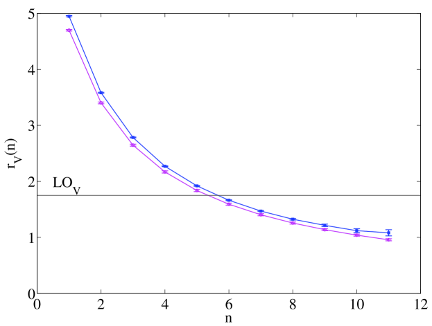
Figure 1: Ratios $r_{\textrm{v}}(n)$ for the static energy on a $8^{4}$ lattice, using TBC in three directions (blue squares) and PBC (magenta circles), respectively.

4 Renormalon observables

So far the only observables that have been checked for a renormalon within NSPT are the plaquette $\langle U_{\square}\rangle$ and small Wilson loops [13, 14, 15, 16, 17]. The factorial growth of the coefficients $w_{n}$ in the expansion,

$$\langle U_{\square}\rangle=\sum_{n=0}^{\infty}w_{n}\alpha^{n+1\,},$$ (11)

translates into the leading-order expectation (see e.g. ref. [1] and eq. (2)),

$$\mathrm{LO_{\mathrm{W}}}=\lim_{n\to\infty}r_{\textrm{w}}(n):=\lim_{n\to\infty}\frac{|w_{n}|}{n|w_{n-1}|}=|a_{4}|=\frac{11}{8\pi}\,.$$ (12)

The static energy $V_{\mathrm{self}}$ which we focus on can be extracted from gauge-invariant Polyakov loop expectation values $\langle P\rangle$ wrapping around the $T$ direction of an $L^{3}\cdot T$ lattice:

$$V_{\mathrm{self}}=\lim_{T\to\infty}\left(-\frac{1}{T}\mathrm{ln}\,\langle P\rangle\right)\,.$$ (13)

The self-energy of a static quark is linearly UV-divergent. Hence, the perturbative coefficients $v_{n}$ of the expansion of $V_{\mathrm{self}}$ are expected to be sensitive to a leading UV renormalon at $u=1/2$: the leading-order expectation reads [18, 19, 20],

$$\mathrm{LO_{\mathrm{V}}}=\lim_{n\to\infty}r_{\textrm{v}}(n)=\lim_{n\to\infty}\frac{|v_{n}|}{n|v_{n-1}|}=\frac{11}{2\pi}=4\,\mathrm{LO_{\mathrm{W}}},$$ (14)

5 Preliminary results

Ref. [21] triggered our interest in combining the static energy calculation with TBC. In this reference the static energy was calculated for various lattice sizes at first and second order. TBC in three spatial directions (TBC3) and even more so TBC in two spatial directions (TBC2) were found to approach the infinite-volume values much faster than PBC. We ran simulations up to $O(\alpha^{12})$ and confirm these findings at higher orders. In fig. 1 we employ both TBC3 and PBC to calculate the static energy on an $8^{4}$ lattice volume, resulting in two sets of ratios $r_{\textrm{v}}(n)$, see eq. (14). For large $n$, the TBC3 ratios lie significantly closer to $\mathrm{LO_{\mathrm{V}}}$ than the PBC ratios.

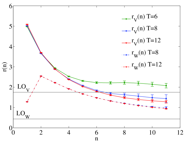
Figure 2: Ratios $r_{\textrm{v}}(n)$ for the static energy from lattice volumes $6^{4}$ (green sqares), $6^{3}\cdot 8$ (blue circles) and $6^{3}\cdot 12$ (red triangles). For the latter two lattice volumes also the plaquette ratios $r_{\textrm{w}}(n)$ are shown (dashed-dotted lines).

We kept the spatial volume fixed to $L^{3}=6^{3}$ to test the viability of eq. (13) at finite $T=6,8,12$. Fig. 2 illustrates that the ratio curve drops significantly when increasing $T$ from $T=6$ to $T=8$. Obviously, $T=6$ does not yet probe the large-$T$ limit. In contrast, the $T=12$ ratios agree within errors with the $T=8$ data, indicating the onset of convergence towards the static energy and its renormalon. Fig. 2 also includes the plaquette ratios for $T=8$ and $T=12$ and these practically coincide. This milder volume dependence for this more localized quantity seems very plausible. We point out the clear separation between plaquette and static energy ratios. Since the renormalon dominance of $V_{\mathrm{self}}$ only starts around the order $n\approx 8$, we would not expect the plaquette ratios to saturate at their asymptotic value for $n<30$.

We also implemented stout smearing for the temporal links (once, with smearing parameter $\rho=1/6$) and calculated eq. (13) in the adjoint representation. The outcome is presented in fig. 3 for the TBC2 simulation on the $6^{3}\cdot 12$ volume. We find that, as far as a potential renormalon is concerned, smearing only affects low ($n=1,2$) perturbative orders, while higher-order ratios collapse onto the unsmeared values. Similarly, the change in representation makes no difference regarding the renormalon position. The adjoint coefficients at large orders are also interesting in view of Casimir scaling violations [2, 22].

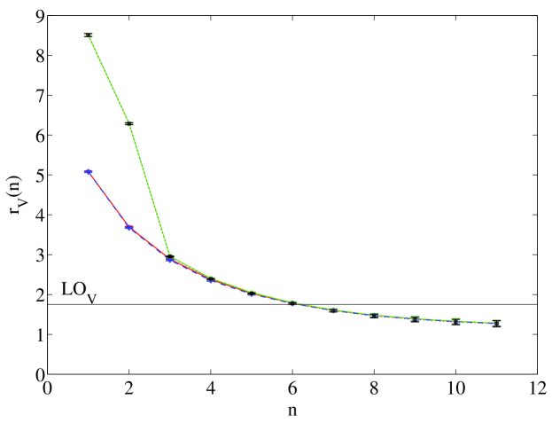
Figure 3: Ratios $r_{\textrm{v}}(n)$ on a $6^{3}\cdot 12$ lattice. Again we plot the static energy, with (green, solid) and without stout smearing (red,solid). In addition, the static energy in the adjoint representation is shown with (black, dotted) and without smearing (blue, dashed).

6 Summary

The perturbative static energy is expected to sense a leading renormalon emerging four times faster than its plaquette counterpart. In an exploratory study we have calculated the static energy from Polyakov loops in NSPT up to $O(\alpha^{12})$ on small lattice volumes, where the use of TBC has proven to drastically reduce finite-size effects. Given the lattice sizes we used and the fact that theoretical predictions are within range, we are confident that our ongoing large-volume simulations will shed more light on the static energy renormalon.

- [1] M. Beneke, Phys. Rept. 317 (1999) 001 [arXiv:hep-ph/9807443].
- [2] C. Anzai, Y. Kiyo and Y. Sumino, Nucl. Phys. B 838 (2010) 28 [arXiv:1004.1562 [hep-ph]].
- [3] T. van Ritbergen, J. A. M. Vermaseren and S. A. Larin, Phys. Lett. B 400 (1997) 379 [arXiv:hep-ph/9701390].
- [4] F. Di Renzo, G. Marchesini, P. Marenzoni and E. Onofri, Nucl. Phys. Proc. Suppl. 34 (1994) 795.
- [5] F. Di Renzo, E. Onofri, G. Marchesini and P. Marenzoni, Nucl. Phys. B 426 (1994) 675 [arXiv:hep-lat/9405019].
- [6] G. Parisi and Y.-S. Wu, Sci. Sin. 24 (1981) 483.
- [7] F. Di Renzo and L. Scorzato, JHEP 0410 (2004) 073 [arXiv:hep-lat/0410010].
- [8] C. Torrero and G. S. Bali, PoS LATTICE2008 215 [arXiv:0812.1680 [hep-lat]].
- [9] G. ’t Hooft, Nucl. Phys. B 153 (1979) 141.
- [10] G. Parisi, in Proceedings of Progress in Gauge Field Theory, Cargese, France, September 1983.
- [11] M. Lüscher and P. Weisz, Nucl. Phys. B 266 (1986) 309.
- [12] A. Gonzalez Arroyo and C. P. Korthals Altes, Nucl. Phys. B 311 (1988) 433.
- [13] F. Di Renzo, E. Onofri and G. Marchesini, Nucl. Phys. B 457 (1995) 202 [arXiv:hep-th/9502095].
- [14] F. Di Renzo and L. Scorzato, JHEP 0110 (2001) 038 [arXiv:hep-lat/0011067].
- [15] P. E. L. Rakow, PoS LAT2005 284 [arXiv:hep-lat/0510046].
- [16] H. Perlt et al., PoS LAT2009 236 [arXiv:0910.2795 [hep-lat]].
- [17] R. Horsley et al., these proceedings [arXiv:1010.4674 [hep-lat]].
- [18] M. Beneke and V. M. Braun, Nucl. Phys. B 426 (1994) 301 [arXiv:hep-ph/9402364].
- [19] M. Beneke, Phys. Lett. B 344 (1995) 341 [arXiv:hep-ph/9408380].
- [20] A. Pineda, JHEP 0106 (2001) 022 [arXiv:hep-ph/0105008].
- [21] M. A. Nobes et al., Nucl. Phys. Proc. Suppl. 106 (2002) 838 [arXiv:hep-lat/0110051].
- [22] G. S. Bali and A. Pineda, Phys. Rev. D 69 (2004) 094001 [arXiv:hep-ph/0310130].