Sorting by Transpositions is Difficult

Introduction

Along with reversals, transpositions are one of the most elementary large-scale operations that can affect a genome. A transposition consists in swapping two consecutive sequences of genes or, equivalently, in moving a sequence of genes from one place to another in the genome. The transposition distance between two genomes is the minimum number of such operations that are needed to transform one genome into the other. Computing this distance is a challenge in comparative genomics, since it gives a maximum parsimony evolution scenario between the two genomes.

The Sorting by Transpositions problem is the problem of computing the transposition distance between genomes represented by permutations. Since its introduction by Bafna and Pevzner [3, 4], the complexity class of this problem has never been established. Hence a number of studies [4, 8, 15, 17, 12, 5, 14] aim at designing approximation algorithms or heuristics, the best known fixed-ratio algorithm being a 1.375-approximation [12]. Other works [16, 8, 13, 19, 12, 5] aim at computing bounds on the transposition distance of a permutation. Studies have also been devoted to variants of this problem, by considering, for example, prefix transpositions [11, 20, 7] (in which one of the blocks is a prefix of the sequence), or distance between strings [9, 10, 23, 22, 18] (where multiple occurences of each element are allowed in the sequences), possibly with weighted or prefix transpositions [21, 6, 1, 2, 7].

In this paper, we address the long-standing issue of determining the complexity class of the Sorting by Transpositions problem, by giving a polynomial time reduction from SAT, thus proving the NP-hardness of this problem. Our reduction is based on the study of transpositions removing three breakpoints. A corollary of our result is the NP-hardness of the following problem, introduced by [8]: given a permutation $\pi$, is it possible to sort $\pi$ using $d_{b}(\pi)/3$ permutations, where $d_{b}(\pi)$ is the number of breakpoints of $\pi$?

1 Preliminaries

1.1 Transpositions and Breakpoints

In this paper, $n$ denotes a positive integer. Let $\left\llbracket a\,;\,b\right\rrbracket={\{x\in\mathbb{N}\mid a\leq x\leq b\}}$, and $Id_{n}$ be the identity permutation over $\left\llbracket 0\,;\,n\right\rrbracket$. We consider only permutations of $\left\llbracket 0\,;\,n\right\rrbracket$ such that $0$ and $n$ are fixed-points. Given a word $u_{1}\ u_{2}\ \ldots\ u_{l}$, a subword is a subsequence $u_{p_{1}}\ u_{p_{2}}\ \ldots\ u_{p_{l^{\prime}}}$, where $1\leq p_{1}<p_{2}<\ldots<p_{l^{\prime}}\leq l$. A factor is a subsequence of contiguous elements, i.e. a subword with $p_{k+1}=p_{k}+1$ for every $k\in\left\llbracket 1\,;\,l^{\prime}-1\right\rrbracket$.

A transposition is an operation that exchanges two consecutive factors of a sequence. As we only work with permutations, it is defined as a permutation $\tau_{i,j,k}$, which, once composed to a permutation $\pi$, realise this operation (see Figure 1). The transposition $\tau_{i,j,k}$ is formally defined as follows.

Definition 1 (Transposition).

Given three integers $i,j,k$ such that $0<i<j<k\leq n$, the transposition $\tau_{i,j,k}$ over $\left\llbracket 0\,;\,n\right\rrbracket$ is the following permutation (we write $q(j)=k+i-j$):

$$\text{For any }0\leq x<i, \tau_{i,j,k}(x)=x$$

$$\text{For any }i\leq x<q(j), \tau_{i,j,k}(x)=x+j-i$$

$$\text{For any }q(j)\leq x<k, \tau_{i,j,k}(x)=x+j-k$$

$$\text{For any }k\leq x\leq n, \tau_{i,j,k}(x)=x$$

Note that the inverse function of $\tau_{i,j,k}$ is also a transposition. More precisely, $\tau_{i,j,k}^{-1}=\tau_{i,q(j),k}$.

$$\begin{array}[]{ccc}\pi&=&(\pi_{0}\pi_{1}\ldots\pi_{i-1}\underline{\pi_{i}\ldots\pi_{j-1}}\ \underline{\pi_{j}\quad\ldots\quad\pi_{k-1}}\pi_{k}\ldots\pi_{n})\\ \pi\circ\tau_{i,j,k}&=&(\pi_{0}\pi_{1}\ldots\pi_{i-1}\underline{\pi_{j}\quad\ldots\quad\pi_{k-1}}\ \underline{\pi_{i}\ldots\pi_{j-1}}\pi_{k}\ldots\pi_{n})\end{array}$$

Figure 1: Representation of a transposition $\tau_{i,j,k}$, with $0<i<j<k\leq n$.

The following two properties directly follow from the definition of a transposition:

Property 1.

Let $\tau=\tau_{i,j,k}$ be a transposition, $q(j)=k+i-j$, and $u,v\in\left\llbracket 0\,;\,n\right\rrbracket$ be two integers such that $u<v$. Then:

$$\tau(u)>\tau(v) \Leftrightarrow i\leq u<q(j)\leq v<k$$

$$\tau^{-1}(u)>\tau^{-1}(v) \Leftrightarrow i\leq u<j\leq v<k$$

Property 2.

Let $\tau$ be the transposition $\tau=\tau_{i,j,k}$, and write $q(j)=k+i-j$. For all $x\in\left\llbracket 1\,;\,n\right\rrbracket$, the values of $\tau(x-1)$ and $\tau^{-1}(x-1)$ are the following:

$$\begin{array}[]{lrcl}\forall x\notin\{i,q(j),k\},&\tau(x-1)&=&\tau(x)-1\\ \forall x\notin\{i,j,k\},&\tau^{-1}(x-1)&=&\tau^{-1}(x)-1\end{array}$$

$$\begin{array}[]{rclrcl}\tau(i-1)&=&\tau(q(j))-1&\tau^{-1}(i-1)&=&\tau^{-1}(j)-1\\ \tau(q(j)-1)&=&\tau(k)-1&\tau^{-1}(j-1)&=&\tau^{-1}(k)-1\\ \tau(k-1)&=&\tau(i)-1&\tau^{-1}(k-1)&=&\tau^{-1}(i)-1\\ \end{array}$$

Definition 2 (Breakpoints).

Let $\pi$ be a permutation of $\left\llbracket 0\,;\,n\right\rrbracket$. If $x\in\left\llbracket 1\,;\,n\right\rrbracket$ is an integer such that $\pi(x-1)=\pi(x)-1$, then $(x-1,x)$ is an adjacency of $\pi$, otherwise it is a breakpoint. We write $d_{b}(\pi)$ the number of breakpoints of $\pi$.

The following property yields that the number of breakpoints of a permutation can be reduced by at most 3 when a transposition is applied:

Property 3.

Let $\pi$ be a permutation and $\tau=\tau_{i,j,k}$ be a transposition (with $0<i<j<k\leq n$). Then, for all $x\in\left\llbracket 1\,;\,n\right\rrbracket-\{i,j,k\}$,

$$(x-1,x)\text{ is an adjacency of }\pi\Leftrightarrow(\tau^{-1}(x)-1,\tau^{-1}(x))\text{ is an adjacency of }\pi\circ\tau.$$

Overall, we have $d_{b}(\pi\circ\tau)\geq d_{b}(\pi)-3$.

Proof.

For all $x\in\left\llbracket 1\,;\,n\right\rrbracket-\{i,j,k\}$, we have:

$$(x-1,x)\text{ adjacency of }\pi \Leftrightarrow\pi(x-1)=\pi(x)-1$$

$$\Leftrightarrow\pi(\tau(\tau^{-1}(x-1)))=\pi(\tau(\tau^{-1}(x)))-1$$

$$\Leftrightarrow\pi\circ\tau(\tau^{-1}(x)-1)=\pi\circ\tau(\tau^{-1}(x))-1\text{ by Prop.\leavevmode\nobreak\ \ref{prop:tauXmoinsUn}}$$

$$\Leftrightarrow(\tau^{-1}(x)-1,\tau^{-1}(x))\text{ adjacency of }\pi\circ\tau.$$

∎

1.2 Transposition distance

The transposition distance of a permutation is the minimum number of transpositions needed to transform it into the identity. A formal definition is the following:

Definition 3 (Transposition distance).

Let $\pi$ be a permutation of $\left\llbracket 0\,;\,n\right\rrbracket$. The transposition distance $d_{t}(\pi)$ from $\pi$ to $Id_{n}$ is the minimum value $k$ for which there exist $k$ transpositions $\tau_{1},\tau_{2},\ldots,\tau_{k}$, satisfying:

$$\pi\circ\tau_{k}\circ\ldots\circ\tau_{2}\circ\tau_{1}=Id_{n}$$

The decision problem of computing the transposition distance is the following:

Sorting by Transpositions Problem [3] Input: A permutation $\pi$, an integer $k$. Question: Is $d_{t}(\pi)\leq k$?

The following property directly follows from Property 3, since for any $n$ the number of breakpoints of $Id_{n}$ is $0$.

Property 4.

Let $\pi$ be a permutation, then $d_{t}(\pi)\geq d_{b}(\pi)/3$.

Figure 2 gives an example of the computation of the transposition distance.

$$\begin{array}[]{lcl}\pi&=&0\ \underline{2\ 4}\ \underline{3\ 1}\ 5\\ \pi\circ\tau_{1,3,5}&=&0\ \underline{3}\ \underline{1\ 2}\ 4\ 5\\ \pi\circ\tau_{1,3,5}\circ\tau_{1,2,4}&=&0\ 1\ 2\ 3\ 4\ 5\\ \end{array}$$

Figure 2: The transposition distance from $\pi=(0\ 2\ 4\ 3\ 1\ 5)$ to $Id_{5}$ is $2$: it is at most $2$ since $\pi\circ\tau_{1,3,5}\circ\tau_{1,2,4}=Id_{5}$, and it cannot be less than $2$ since Property 4 applies with $d_{b}(\pi)/3=5/3>1$.

2 3-Deletion and Transposition Operations

In this section, we introduce 3DT-instances, which are the cornerstone of our reduction from SAT to the Sorting by Transpositions problem, since they are used as an intermediate between instances of the two problems. We first define 3DT-instances and the possible operations that can be applied to them, then we focus on the equivalence between these instances and permutations.

2.1 3DT-instances

Definition 4 (3DT-instance).

A 3DT-instance $I=\left<\Sigma,T,\psi\right>$ of span $n$ is composed of the following elements:

• $\Sigma$: an alphabet;

• $T=\{(a_{i},b_{i},c_{i})\mid 1\leq i\leq\left\lvert T\right\rvert\}$: a set of (ordered) triples of elements of $\Sigma$, partitioning $\Sigma$ (i.e. all elements are pairwise distinct, and $\bigcup_{i=1}^{|T|}\{a_{i},b_{i},c_{i}\}=\Sigma$);

• $\psi:\Sigma\rightarrow\left\llbracket 1\,;\,n\right\rrbracket$, an injection.

The domain of $I$ is the image of $\psi$, that is the set $L=\{\psi(\sigma)\mid\sigma\in\Sigma\}$.

The word representation of $I$ is the $n$-letter word $u_{1}\ u_{2}\ldots u_{n}$ over $\Sigma\cup\{\raisebox{1.00006pt}{$\centerdot$}\}$ (where $\raisebox{1.00006pt}{$\centerdot$}\notin\Sigma$), such that for all $i\in L$, $\psi(u_{i})=i$, and for $i\in\left\llbracket 1\,;\,n\right\rrbracket-L$, $u_{i}=\raisebox{1.00006pt}{$\centerdot$}$.

Two examples of 3DT-instances are given in Example 1. Note that such instances can be defined by their word representation and by their set of triples $T$. The empty 3DT-instance, in which $\Sigma=\emptyset$, can be written with a sequence of $n$ dots, or with the empty word $\varepsilon$.

Example 1.

In this example, we define two 3DT-instances of span 6, $I=\left<\Sigma,T,\psi\right>$ and $I^{\prime}=\left<\Sigma^{\prime},T^{\prime},\psi^{\prime}\right>$:

$$\begin{array}[]{lcll}I&=&a_{1}\ c_{2}\ b_{1}\ b_{2}\ c_{1}\ a_{2}&\text{ with }T=\{(a_{1},b_{1},c_{1}),(a_{2},b_{2},c_{2})\}\\ I^{\prime}&=&\;\;\raisebox{1.00006pt}{$\centerdot$}\;\ b_{2}\ \;\raisebox{1.00006pt}{$\centerdot$}\;\ c_{2}\ \;\raisebox{1.00006pt}{$\centerdot$}\;\ a_{2}&\text{ with }T^{\prime}=\{(a_{2},b_{2},c_{2})\}\end{array}$$

Here, $I$ has an alphabet of size 6, $\Sigma=\{a_{1},b_{1},c_{1},a_{2},b_{2},c_{2}\}$, hence $\psi$ is a bijection ($\psi(a_{1})=1$, $\psi(c_{2})=2$, $\psi(b_{1})=3$, etc). The second instance, $I^{\prime}$, has an alphabet of size 3, $\Sigma^{\prime}=\{a_{2},b_{2},c_{2}\}$, with $\psi^{\prime}(b_{2})=2$, $\psi^{\prime}(c_{2})=4$, $\psi^{\prime}(a_{2})=6$.

Property 5.

Let $I=\left<\Sigma,T,\psi\right>$ be a 3DT-instance of span $n$ with domain $L$. Then

$$\left\lvert\Sigma\right\rvert=\left\lvert L\right\rvert=3\left\lvert T\right\rvert\leq n.$$

Proof.

We have $|\Sigma|=|L|$ since $\psi$ is an injection with image $L$. The triples of $T$ partition $\Sigma$ so $|\Sigma|=3|T|$, and finally $L\subseteq\left\llbracket 1\,;\,n\right\rrbracket$ so $|L|\leq n$. ∎

Definition 5.

Let $I=\left<\Sigma,T,\psi\right>$ be a 3DT-instance. The injection $\psi$ gives a total order over $\Sigma$, written $\prec_{I}$ (or $\prec$, if there is no ambiguity), defined by

$$\forall\sigma_{1},\sigma_{2}\in\Sigma,\quad\sigma_{1}\prec_{I}\sigma_{2}\Leftrightarrow\psi(\sigma_{1})<\psi(\sigma_{2})$$ (1)

Two elements $\sigma_{1}$ and $\sigma_{2}$ of $\Sigma$ are called consecutive if there exists no element $x\in\Sigma$ such that $\sigma_{1}\prec_{I}x\prec_{I}\sigma_{2}$. In this case, we write $\sigma_{1}\triangleleft_{I}\sigma_{2}$ (or simply $\sigma_{1}\triangleleft\sigma_{2}$).

An equivalent definition is that $\sigma_{1}\prec\sigma_{2}$ if $\sigma_{1}\ \sigma_{2}$ is a subword of the word representation of $I$. Also, $\sigma_{1}\triangleleft\sigma_{2}$ if the word representation of $I$ contains a factor of the kind $\sigma_{1}\ \raisebox{1.00006pt}{$\centerdot$}^{*}\ \sigma_{2}$ (where $\raisebox{1.00006pt}{$\centerdot$}^{*}$ represents any sequence of $l\geq 0$ dots).

Using the triples in $T$, we define a successor function over the domain $L$:

Definition 6.

Let $I=\left<\Sigma,T,\psi\right>$ be a 3DT-instance with domain $L$. The function $succ_{I}:L\rightarrow L$ is defined by:

$$\forall(a,b,c)\in T,\quad\psi(a) \mapsto\psi(b)$$

$$\psi(b) \mapsto\psi(c)$$

$$\psi(c) \mapsto\psi(a)$$

Function $succ_{I}$ is a bijection, with no fixed-points, and such that $succ_{I}\circ succ_{I}\circ succ_{I}$ is the identity over $L$. In Example 1, we have:

$$succ_{I}=\left(\begin{matrix}1&2&3&4&5&6\\ 3&6&5&2&1&4\end{matrix}\right)\text{\ and \ }succ_{I^{\prime}}=\left(\begin{matrix}2&4&6\\ 4&6&2\end{matrix}\right).$$

2.2 3DT-steps

Definition 7.

Let $I=\left<\Sigma,T,\psi\right>$ be a 3DT-instance, and $(a,b,c)$ be a triple of $T$. Write $i=\min\{\psi(a),\psi(b),\psi(c)\}$, $j=succ_{I}(i)$, and $k=succ_{I}(j)$. The triple $(a,b,c)\in T$ is well-ordered if we have $i<j<k$. In such a case, we write $\tau[a,b,c,\psi]$ the transposition $\tau_{i,j,k}$.

An equivalent definition is that $(a,b,c)$ is well-ordered iff one of $abc$, $bca$, $cab$ is a subword of the word representation of $I$. In Example 1, $(a_{1},b_{1},c_{1})$ is well-ordered in $I$: indeed, we have $i=\psi(a_{1})$, $j=\psi(b_{1})$ and $k=\psi(c_{1})$, so $i<j<k$. The triple $(a_{2},b_{2},c_{2})$ is also well-ordered in $I^{\prime}$ ($i=\psi^{\prime}(b_{2})<j=\psi^{\prime}(c_{2})<k=\psi^{\prime}(a_{2})$), but not in $I$: $i=\psi(c_{2})<k=\psi(b_{2})<j=\psi(a_{2})$. In this example, we have $\tau[a_{1},b_{1},c_{1},\psi]=\tau_{1,3,5}$ and $\tau[a_{2},b_{2},c_{2},\psi^{\prime}]=\tau_{2,4,6}$.

Definition 8 (3DT-step).

Let $I=\left<\Sigma,T,\psi\right>$ be a 3DT-instance with $(a,b,c)\in T$ a well-ordered triple. The 3DT-step of parameter $(a,b,c)$ is the operation written $\underrightarrow{\;(a,b,c)\;}$, transforming $I$ into the 3DT-instance $I^{\prime}=\left<\Sigma^{\prime},T^{\prime},\psi^{\prime}\right>$ such that:

• $\Sigma^{\prime}=\Sigma-\{a,b,c\}$

• $T^{\prime}=T-\{(a,b,c)\}$

• $\psi^{\prime}:\begin{array}[]{ccc}\Sigma^{\prime}&\rightarrow&\left\llbracket 1\,;\,n\right\rrbracket\\ \sigma&\mapsto&\tau^{-1}(\psi(\sigma))\end{array}$ $($with $\tau=\tau[a,b,c,\psi])$.

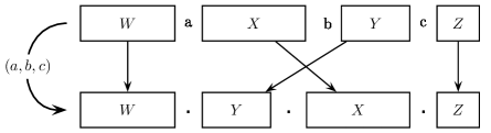
Figure 3: The 3DT-step $\underrightarrow{\;(a,b,c)\;}$ has two effects, here represented on the word representation of a 3DT-instance: the triple $(a,b,c)$ is deleted (and replaced by dots in this word representation), and the factors $X$ and $Y$ are swapped.

A 3DT-step has two effects on a 3DT-instance, as represented in Figure 3. The first is to remove a necessarily well-ordered triple from $T$ (hence from $\Sigma$). The second is, by applying a transposition to $\psi$, to shift the position of some of the remaining elements. Note that a triple that is not well-ordered in $I$ can become well-ordered in $I^{\prime}$, or vice-versa. In Example 1, $I^{\prime}$ can be obtained from $I$ via a 3DT-step: $I\raisebox{5.0pt}{\scriptsize$\underrightarrow{\;(a_{1},b_{1},c_{1})\;}$}I^{\prime}$. Moreover, $I^{\prime}\raisebox{5.0pt}{\scriptsize$\underrightarrow{\;(a_{2},b_{2},c_{2})\;}$}\varepsilon$. A more complex example is given in Figure 4.

Note that a 3DT-step transforms the function $succ_{I}$ into $succ_{I^{\prime}}=\tau^{-1}\circ succ_{I}\circ\tau$, restricted to $L^{\prime}$, the domain of the new instance $I^{\prime}$. Indeed, for all $(a,b,c)\in T^{\prime}$, we have

$$succ_{I^{\prime}}(\psi^{\prime}(a)) =\psi^{\prime}(b)$$

$$=\tau^{-1}(\psi(b))$$

$$=\tau^{-1}(succ_{I}(\psi(a)))$$

$$=\tau^{-1}(succ_{I}(\tau(\psi^{\prime}(a))))$$

$$=(\tau^{-1}\circ succ_{I}\circ\tau)(\psi^{\prime}(a))$$

The computation is similar for $\psi^{\prime}(b)$ and $\psi^{\prime}(c)$.

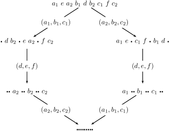
Figure 4: Possible 3DT-steps from the instance $I$ defined by the word $a_{1}\ e\ a_{2}\ b_{1}\ d\ b_{2}\ c_{1}\ f\ c_{2}$ and the set of triples $T=\{(a_{1},b_{1},c_{1}),(a_{2},b_{2},c_{2}),(d,e,f)\}$. We can see that there is a path from $I$ to $\varepsilon$, hence $I$ is 3DT-collapsible. Note that both $(a_{1},b_{1},c_{1})$ and $(a_{2},b_{2},c_{2})$ are well-ordered in the initial instance, each one loses this property after applying the 3DT-step associated to the other, and becomes well-ordered again after applying the 3DT-step associated to $(d,e,f)$.

Definition 9 (3DT-collapsibility).

A 3DT-instance $I=\left<\Sigma,T,\psi\right>$ is 3DT-collapsible if there exists a sequence of 3DT-instances $I_{k},I_{k-1},\ldots,I_{0}$ such that

$$I_{k}=I$$

$$\forall i\in\left\llbracket 1\,;\,k\right\rrbracket,\quad\exists(a,b,c)\in T,\quad I_{i}\raisebox{5.0pt}{\scriptsize$\underrightarrow{\;(a,b,c)\;}$}I_{i-1}$$

$$I_{0}=\varepsilon$$

In Example 1, $I$ and $I^{\prime}$ are 3DT-collapsible, since $I\raisebox{5.0pt}{\scriptsize$\underrightarrow{\;(a_{1},b_{1},c_{1})\;}$}I^{\prime}\raisebox{5.0pt}{\scriptsize$\underrightarrow{\;(a_{2},b_{2},c_{2})\;}$}\varepsilon$. Another example is the 3DT-instance defined in Figure 4. Note that in the example of Figure 4, there are in fact two distinct paths leading to the empty instance.

2.3 Equivalence with the transposition distance

Definition 10.

Let $I=\left<\Sigma,T,\psi\right>$ be a 3DT-instance of span $n$ with domain $L$, and $\pi$ be a permutation of $\left\llbracket 0\,;\,n\right\rrbracket$. We say that $I$ and $\pi$ are equivalent, and we write $I\sim\pi$, if:

$$\begin{array}[]{lrl}&\pi(0)&=0,\\ \forall v\in\left\llbracket 1\,;\,n\right\rrbracket-L,&\pi(v)&=\pi(v-1)+1,\\ \forall v\in L,&\pi(v)&=\pi(succ_{I}^{-1}(v)-1)+1.\end{array}$$

With such an equivalence $I\sim\pi$, the two following properties hold:

• The breakpoints of $\pi$ correspond to the elements of $L$ (see Property 6).

• The triples of breakpoints that may be resolved immediately by a single transposition correspond to the well-ordered triples of $T$ (see Figure 5 and Lemma 8).

Figure 5: Illustration of the equivalence $I\sim\pi$ on three integers $(i,j,k)$ such that $j=succ_{I}(i)$ and $k=succ_{I}(j)$. It can be checked that $\pi(v)=\pi(u-1)+1$ for any $(u,v)\in\{(i,j),(j,k),(k,i)\}$.

Property 6.

Let $I=\left<\Sigma,T,\psi\right>$ be a 3DT-instance of span $n$ with domain $L$, and $\pi$ be a permutation of $\left\llbracket 0\,;\,n\right\rrbracket$, such that $I\sim\pi$. Then the number of breakpoints of $\pi$ is $d_{b}(\pi)=\lvert L\rvert=3|T|$.

Proof.

Let $v\in\left\llbracket 1\,;\,n\right\rrbracket$. By Definition 10, we have:

If $v\notin L$, then $\pi(v)=\pi(v-1)+1$, so $(v-1,v)$ is an adjacency of $\pi$.

If $v\in L$, we write $u=succ_{I}^{-1}(v)$, so $\pi(v)=\pi(u-1)+1$. Since $succ_{I}$ has no fixed-point, we have $u\neq v$, which implies $\pi(u-1)\neq\pi(v-1)$. Hence, $\pi(v)\neq\pi(v-1)+1$, and $(v-1,v)$ is a breakpoint of $\pi$.

Consequently the number of breakpoints of $\pi$ is exactly $\lvert L\rvert$, and $\lvert L\rvert=3|T|$ by Property 5. ∎

Figure 6: Illustration of Lemma 7: since $I\sim\pi$ and $I\raisebox{5.0pt}{\scriptsize$\underrightarrow{\;(a_{1},b_{1},c_{1})\;}$}I^{\prime}$, then $I^{\prime}\sim\pi^{\prime}=\pi\circ\tau$, where $\tau=\tau[a_{1},b_{1},c_{1},\psi]$.

With the following lemma, we show that the equivalence between a 3DT-instance and a permutation is preserved after a 3DT-step, see Figure 6.

Lemma 7.

Let $I=\left<\Sigma,T,\psi\right>$ be a 3DT-instance of span $n$, and $\pi$ be a permutation of $\left\llbracket 0\,;\,n\right\rrbracket$, such that $I\sim\pi$. If there exists a 3DT-step $I\raisebox{5.0pt}{\scriptsize$\underrightarrow{\;(a,b,c)\;}$}I^{\prime}$, then $I^{\prime}$ and $\pi^{\prime}=\pi\circ\tau$, where $\tau=\tau[a,b,c,\psi]$, are equivalent.

Proof.

We write $(i,j,k)$ the indices such that $\tau=\tau_{i,j,k}$ (i.e. $i=\min\{\psi(a),\psi(b),\psi(c)\}$, $j=succ_{I}(i)$, $k=succ_{I}(j)$). Since $(a,b,c)$ is well-ordered, we have $i<j<k$.

We have $I^{\prime}=\left<\Sigma^{\prime},T^{\prime},\psi^{\prime}\right>$, with $\Sigma^{\prime}=\Sigma-\{a,b,c\}$, $T^{\prime}=T-\{(a,b,c)\}$, and $\psi^{\prime}:\sigma\mapsto\tau^{-1}(\psi(\sigma))$. We write respectively $L$ and $L^{\prime}$ the domains of $I$ and $I^{\prime}$. For all $v^{\prime}\in\left\llbracket 1\,;\,n\right\rrbracket$, we have

$$v^{\prime}\in L^{\prime} \Leftrightarrow \exists\sigma\in\Sigma-\{a,b,c\},\ v^{\prime}=\tau^{-1}(\psi(\sigma))$$

$$\Leftrightarrow \tau(v^{\prime})\in L-\{i,j,k\}$$

We prove the 3 required properties (see Definition 10) sequentially:

• $\pi^{\prime}(0)=\pi(\tau(0))=\pi(0)=0$,

• $\forall v^{\prime}\in\left\llbracket 1\,;\,n\right\rrbracket-L^{\prime}$, let $v=\tau(v^{\prime})$. Since $v^{\prime}\notin L^{\prime}$, we have either $v\in\{i,j,k\}$, or $v\notin L$. In the first case, we write $u=succ_{I}^{-1}(v)$ (then $u\in\{i,j,k\}$). By Property 2, $\tau^{-1}(u-1)$ is equal to $\tau^{-1}(succ_{I}(u))-1$, so $\tau^{-1}(u-1)=\tau^{-1}(v)-1$. Hence,

  $$\pi^{\prime}(v^{\prime}-1)+1 =\pi(\tau(\tau^{-1}(v)-1))+1$$

  $$=\pi(u-1)+1$$

  $$=\pi(v)\text{ by Def.\leavevmode\nobreak\ \ref{def:equiv}, since }v\in L\text{ and }v=succ_{I}(u)$$

  $$=\pi^{\prime}(v^{\prime})$$

  In the second case, $v\notin L$, we have

  $$\pi^{\prime}(v^{\prime}-1)+1 =\pi(\tau(\tau^{-1}(v)-1))+1$$

  $$=\pi(\tau(\tau^{-1}(v-1)))+1\text{ by Prop.\leavevmode\nobreak\ \ref{prop:tauXmoinsUn}, since }v\notin\{i,j,k\}$$

  $$=\pi(v-1)+1$$

  $$=\pi(v)\text{ by Def.\leavevmode\nobreak\ \ref{def:equiv}, since }v\notin L$$

  $$=\pi^{\prime}(v^{\prime})$$

  In both cases, we indeed have $\pi^{\prime}(v^{\prime}-1)+1=\pi^{\prime}(v^{\prime})$.

• Let $v^{\prime}$ be an element of $L^{\prime}$. We write $v=\tau(v^{\prime})$, $u=succ_{I}^{-1}(v)$, and $u^{\prime}=\tau^{-1}(u)$. Then $v^{\prime}=\tau^{-1}(succ_{I}(\tau(u^{\prime})))=succ_{I^{\prime}}(u^{\prime})$. Moreover, $v\notin\{i,j,k\}$, hence $u\notin\{i,j,k\}$.

  $$\pi^{\prime}(u^{\prime}-1)+1 =\pi(\tau(\tau^{-1}(u)-1))+1$$

  $$=\pi(\tau(\tau^{-1}(u-1)))+1\text{ by Prop.\leavevmode\nobreak\ \ref{prop:tauXmoinsUn}, since }u\notin\{i,j,k\}$$

  $$=\pi(u-1)+1$$

  $$=\pi(v)\text{ by Def.\leavevmode\nobreak\ \ref{def:equiv}, since }v\in L\text{ and }u=succ_{I}^{-1}(v)$$

  $$=\pi(\tau(\tau^{-1}(v)))$$

  $$=\pi^{\prime}(v^{\prime})$$

∎

Lemma 8.

Let $I=\left<\Sigma,T,\psi\right>$ be a 3DT-instance of span $n$, and $\pi$ a permutation of $\left\llbracket 0\,;\,n\right\rrbracket$, such that $I\sim\pi$. If there exists a transposition $\tau=\tau_{i,j,k}$ such that $d_{b}(\pi\circ\tau)=d_{b}(\pi)-3$, then $T$ contains a well-ordered triple $(a,b,c)$ such that $\tau=\tau[a,b,c,\psi]$.

Proof.

We write $i^{\prime}=\tau^{-1}(i)$, $j^{\prime}=\tau^{-1}(j)$, and $k^{\prime}=\tau^{-1}(k)$. Note that $i<j<k$.

Let $\pi^{\prime}=\pi\circ\tau$. For all $x\in\left\llbracket 1\,;\,n\right\rrbracket-\{i,j,k\}$, we have, by Property 3, that $(x-1,x)$ is an adjacency of $\pi$ iff $(\tau^{-1}(x)-1,\tau^{-1}(x))$ is an adjacency of $\pi^{\prime}$. Hence, since $d_{b}(\pi^{\prime})=d_{b}(\pi)-3$, we necessarily have that $(i-1,i)$, $(j-1,j)$ and $(k-1,k)$ are breakpoints of $\pi$, and $(i^{\prime}-1,i^{\prime})$, $(j^{\prime}-1,j^{\prime})$ and $(k^{\prime}-1,k^{\prime})$ are adjacencies of $\pi^{\prime}$. We have

$$\pi(i) =\pi(\tau(i^{\prime}))$$

$$=\pi^{\prime}(i^{\prime})$$

$$=\pi^{\prime}(i^{\prime}-1)+1\text{ since $(i^{\prime}-1,i^{\prime})$ is an adjacency of $\pi^{\prime}$}$$

$$=\pi^{\prime}(\tau^{-1}(i)-1)+1$$

$$=\pi^{\prime}(\tau^{-1}(k-1))+1\text{ by Prop.\leavevmode\nobreak\ \ref{prop:tauXmoinsUn}}$$

$$=\pi(k-1)+1$$

Since $I\sim\pi$ and $i\neq k$, by Definition 10, we necessarily have $i\in L$ (where $L$ is the domain of $I$), and $i=succ_{I}(k)$.

Using the same method with $(j^{\prime}-1,j^{\prime})$ and $(k^{\prime}-1,k^{\prime})$, we obtain $j,k\in L$, $j=succ_{I}(i)$ and $k=succ_{I}(j)$. Hence, $T$ contains one of the following three triples: $(\psi^{-1}(i),\psi^{-1}(j),\psi^{-1}(k))$, $(\psi^{-1}(j),\psi^{-1}(k),\psi^{-1}(i))$ or $(\psi^{-1}(k),\psi^{-1}(i),\psi^{-1}(j))$. Writing $(a,b,c)$ this triple, we indeed have $\tau_{i,j,k}=\tau[a,b,c,\psi]$ since $i<j<k$. ∎

Theorem 9.

Let $I=\left<\Sigma,T,\psi\right>$ be a 3DT-instance of span $n$ with domain $L$, and $\pi$ be a permutation of $\left\llbracket 0\,;\,n\right\rrbracket$, such that $I\sim\pi$. Then $I$ is 3DT-collapsible if and only if $d_{t}(\pi)=|T|=d_{b}(\pi)/3$.

Proof.

We prove the theorem by induction on $k=|T|$. For $k=0$, necessarily $I=\varepsilon$ and $L=T=\emptyset$, and by Definition 10, $\pi=Id_{n}$ ($\pi(0)=0$, and for all $v>0$, $\pi(v)=\pi(v-1)+1$). In this case, $I$ is trivially 3DT-collapsible, and $d_{t}(\pi)=0=|T|=d_{b}(\pi)/3$.

Suppose now $k=k^{\prime}+1$, with $k^{\prime}\geq 0$, and the theorem is true for $k^{\prime}$. By Property 6, we have $d_{b}(\pi)=3k$, and by Property 4, $d_{t}(\pi)\geq 3k/3=k$.

Assume first that $I$ is 3DT-collapsible. Then there exist both a triple $(a,b,c)\in T$ and a 3DT-instance $I^{\prime}=\left<\Sigma^{\prime},T^{\prime},\psi^{\prime}\right>$ such that $I\raisebox{5.0pt}{\scriptsize$\underrightarrow{\;(a,b,c)\;}$}I^{\prime}$, and that $I^{\prime}$ is 3DT-collapsible. Since $T^{\prime}=T-\{(a,b,c)\}$, the size of $T^{\prime}$ is $k-1=k^{\prime}$. By Lemma 7, we have $I^{\prime}\sim\pi^{\prime}=\pi\circ\tau$, with $\tau=\tau[a,b,c,\psi]$. Using the induction hypothesis, we know that $d_{t}(\pi^{\prime})=k^{\prime}$. So the transposition distance from $\pi=\pi^{\prime}\circ\tau^{-1}$ to the identity is at most, hence exactly, $k^{\prime}+1=k$.

Assume now that $d_{t}(\pi)=k$. We can decompose $\pi$ into $\pi=\pi^{\prime}\circ\tau^{-1}$, where $\tau$ is a transposition and $\pi^{\prime}$ a permutation such that $d_{t}(\pi^{\prime})=k-1=k^{\prime}$. Since $\pi$ has $3k$ breakpoints (Property 6), and $\pi^{\prime}=\pi\circ\tau$ has at most $3k-3$ breakpoints (Property 4), $\tau$ necessarily removes $3$ breakpoints, and we can use Lemma 8: there exists a 3DT-step $I\raisebox{5.0pt}{\scriptsize$\underrightarrow{\;(a,b,c)\;}$}I^{\prime}$, where $(a,b,c)\in T$ is a well-ordered triple and $\tau=\tau[a,b,c,\psi]$. We can now use Lemma 7, which yields $I^{\prime}\sim\pi^{\prime}=\pi\circ\tau$. Using the induction hypothesis, we obtain that $I^{\prime}$ is 3DT-collapsible, hence $I$ is also 3DT-collapsible. This concludes the proof of the theorem. ∎

The previous theorem gives a way to reduce the problem of deciding if a 3DT-instance is collapsible to the Sorting by Transpositions problem. However, it must be used carefully, since there exist 3DT-instances to which no permutation is equivalent (for example, $I=a_{1}\ a_{2}\ b_{1}\ b_{2}\ c_{1}\ c_{2}$ admits no permutation $\pi$ of $\left\llbracket 0\,;\,6\right\rrbracket$ such that $I\sim\pi$).

3 3DT-collapsibility is NP-Hard to Decide

In this section, we define, for any boolean formula $\phi$, a corresponding 3DT-instance $I_{\phi}$. We also prove that $I_{\phi}$ is 3DT-collapsible if and only if $\phi$ is satisfiable.

3.1 Block Structure

The construction of the 3DT-instance $I_{\phi}$ uses a decomposition into blocks, defined below. Some triples will be included in a block, in order to define its behavior, while others will be shared between two blocks, in order to pass information. The former are unconstrained, so that we can design blocks with the behavior we need (for example, blocks mimicking usual boolean functions), while the latter need to follow several rules, so that the blocks can conveniently be arranged together.

Definition 11 ($l$-block-decomposition).

An $l$-block-decomposition $\mathcal{B}$ of a 3DT-instance $I$ of span $n$ is an $l$-tuple $(s_{1},\ldots,s_{l})$ such that $s_{1}=0$, for all $h\in\left\llbracket 1\,;\,l-1\right\rrbracket$, $s_{h}<s_{h+1}$ and $s_{l}<n$. We write $t_{h}=s_{h+1}$ for $h\in\left\llbracket 1\,;\,l-1\right\rrbracket$, and $t_{l}=n$.

Let $I=\left<\Sigma,T,\psi\right>$. For $h\in\left\llbracket 1\,;\,l\right\rrbracket$, the factor $u_{s_{h}+1}\ u_{s_{h}+2}\ \ldots u_{t_{h}}$ of the word representation $u_{1}\ u_{2}\ \ldots u_{n}$ of $I$ is called the full block $\mathcal{B}^{\raisebox{0.70004pt}{$\centerdot$}}_{h}$ (it is a word over $\Sigma\cup\{\raisebox{1.00006pt}{$\centerdot$}\}$). The subword of $\mathcal{B}^{\raisebox{0.70004pt}{$\centerdot$}}_{h}$ where every occurrence of $\centerdot$ is deleted is called the block $\mathcal{B}_{h}$.

For $\sigma\in\Sigma$, we write $block_{I,\mathcal{B}}(\sigma)=h$ if $\psi(\sigma)\in\left\llbracket s_{h}+1\,;\,t_{h}\right\rrbracket$ (equivalently, if $\sigma$ appears in the word $\mathcal{B}_{h}$). A triple $(a,b,c)\in T$ is said to be internal if $block_{I,\mathcal{B}}(a)=block_{I,\mathcal{B}}(b)=block_{I,\mathcal{B}}(c)$, external otherwise.

If $\tau$ is a transposition such that for all $h\in\left\llbracket 1\,;\,l\right\rrbracket$, $\tau(s_{h})<\tau(t_{h})$, we write $\tau[\mathcal{B}]$ the $l$-block-decomposition $(\tau(s_{1}),\ldots,\tau(s_{l}))$.

In the rest of this section, we mostly work with blocks instead of full blocks, since we are only interested in the relative order of the elements, rather than their actual position. Full blocks are only used in definitions, where we want to control the dots in the word representation of the 3DT-instances we define. Note that, for $\sigma_{1},\sigma_{2}\in\Sigma$ such that $block_{I,\mathcal{B}}(\sigma_{1})=block_{I,\mathcal{B}}(\sigma_{2})=h$, the relation $\sigma_{1}\triangleleft\sigma_{2}$ is equivalent to $\sigma_{1}\ \sigma_{2}$ is a factor of $\mathcal{B}_{h}$.

Property 10.

Let $\mathcal{B}=(s_{1},\ldots,s_{l})$ be an $l$-block-decomposition of a 3DT-instance of span $n$, and $i,j,k\in\left\llbracket 1\,;\,n\right\rrbracket$ be three integers such that (a) $i<j<k$ and (b) $\exists{h_{0}}$ such that $s_{h_{0}}<i<j\leq t_{h_{0}}$ or $s_{h_{0}}<j<k\leq t_{h_{0}}$ (or both). Then for all $h\in\left\llbracket 1\,;\,l\right\rrbracket$, $\tau_{i,j,k}^{-1}(s_{h})<\tau_{i,j,k}^{-1}(t_{h})$, and the $l$-block-decomposition $\tau_{i,j,k}^{-1}[\mathcal{B}]$ is defined.

Proof.

For any $h\in\left\llbracket 1\,;\,l\right\rrbracket$, we show that we cannot have $i\leq s_{h}<j\leq t_{h}<k$. Indeed, $s_{h}<j$ implies $h\leq h_{0}$ (since $s_{h}<j\leq t_{h_{0}}=s_{h_{0}+1}$), and $j\leq t_{h}$ implies $h\geq h_{0}$ (since $t_{h_{0}-1}=s_{h_{0}}<j\leq t_{h}$). Hence $s_{h}<j\leq t_{h}$ implies $h=h_{0}$, but $i\leq s_{h},t_{h}<k$ contradicts both conditions $s_{h_{0}}<i$ and $k\leq t_{h_{0}}$: hence the relation $i\leq s_{h}<j\leq t_{h}<k$ is impossible.

By Property 1, since $s_{h}<t_{h}$ for all $h\in\left\llbracket 1\,;\,l\right\rrbracket$, and $i\leq s_{h}<j\leq t_{h}<k$ does not hold, we have $\tau_{i,j,k}^{-1}(s_{h})<\tau_{i,j,k}^{-1}(t_{h})$, which is sufficient to define $\tau_{i,j,k}^{-1}[\mathcal{B}]$. ∎

The above property yields that, if $(a,b,c)$ is a well-ordered triple of a 3DT-instance $I=\left<\Sigma,T,\psi\right>$ ($\tau=\tau[a,b,c,\psi]$), and $\mathcal{B}$ is an $l$-block-decomposition of $I$, then $\tau^{-1}[\mathcal{B}]$ is defined if $(a,b,c)$ is an internal triple, or an external triple such that one of the following equalities is satisfied: $block_{I,\mathcal{B}}(a)=block_{I,\mathcal{B}}(b)$, $block_{I,\mathcal{B}}(b)=block_{I,\mathcal{B}}(c)$ or $block_{I,\mathcal{B}}(c)=block_{I,\mathcal{B}}(a)$. In this case, the 3DT-step $I\raisebox{5.0pt}{\scriptsize$\underrightarrow{\;(a,b,c)\;}$}I^{\prime}$ is written $(I,\mathcal{B})\raisebox{5.0pt}{\scriptsize$\underrightarrow{\;(a,b,c)\;}$}(I^{\prime},\mathcal{B}^{\prime})$, where $\mathcal{B}^{\prime}=\tau^{-1}[\mathcal{B}]$ is an $l$-block-decomposition of $I^{\prime}$.

Definition 12 (Variable).

A variable $A$ of a 3DT-instance $I=\left<\Sigma,T,\psi\right>$ is a pair of triples $A=[(a,b,c),(x,y,z)]$ of $T$. It is valid in an $l$-block-decomposition $\mathcal{B}$ if

• $\exists h_{0}\in\left\llbracket 1\,;\,l\right\rrbracket$ such that $block_{I,\mathcal{B}}(b)=block_{I,\mathcal{B}}(x)=block_{I,\mathcal{B}}(y)=h_{0}$

• $\exists h_{1}\in\left\llbracket 1\,;\,l\right\rrbracket$, $h_{1}\neq h_{0}$, such that $block_{I,\mathcal{B}}(a)=block_{I,\mathcal{B}}(c)=block_{I,\mathcal{B}}(z)=h_{1}$

• if $x\prec y$, then we have $x\triangleleft b\triangleleft y$

• $a\prec z\prec c$

For such a valid variable $A$, the block $\mathcal{B}_{h_{0}}$ containing $\{b,x,y\}$ is called the source of $A$ (we write $source(A)={h_{0}}$), and the block $\mathcal{B}_{h_{1}}$ containing $\{a,c,z\}$ is called the target of $A$ (we write $target(A)={h_{1}}$). For $h\in\left\llbracket 1\,;\,l\right\rrbracket$, the variables of which $\mathcal{B}_{h}$ is the source (resp. the target) are called the output (resp. the input) of $\mathcal{B}_{h}$. The 3DT-step $I\raisebox{5.0pt}{\scriptsize$\underrightarrow{\;(x,y,z)\;}$}I^{\prime}$ is called the activation of $A$ (it requires that $(x,y,z)$ is well-ordered).

Note that since a valid variable $A=[(a,b,c),(x,y,z)]$ has $block_{I,\mathcal{B}}(x)=block_{I,\mathcal{B}}(y)$, its activation can be written $(I,\mathcal{B})\raisebox{5.0pt}{\scriptsize$\underrightarrow{\;(x,y,z)\;}$}(I^{\prime},\mathcal{B}^{\prime})$.

Property 11.

Let $(I,\mathcal{B})$ be a 3DT-instance with an $l$-block-decomposition, and $A$ be a variable of $I$ that is valid in $\mathcal{B}$. Write $A=[(a,b,c),(x,y,z)]$. Then $(x,y,z)$ is well-ordered iff $x\prec y$; and $(a,b,c)$ is not well-ordered.

Proof.

Note that for all $\sigma,\sigma^{\prime}\in\Sigma$, $block_{I,\mathcal{B}}(\sigma)<block_{I,\mathcal{B}}(\sigma^{\prime})\Rightarrow\sigma\prec\sigma^{\prime}$. Write $I=\left<\Sigma,T,\psi\right>$, ${h_{0}}=source(A)$ and ${h_{1}}=target(A)$: we have $h_{0}\neq h_{1}$ by condition (ii) of Definition 12.

If ${h_{0}}<{h_{1}}$, then, with condition (iv) of Definition 12, $b\prec a\prec c$, and either $x\prec y\prec z$ or $y\prec x\prec z$. Hence, $(a,b,c)$ is not well-ordered, and $(x,y,z)$ is well-ordered iff $x\prec y$.

Likewise, if ${h_{1}}<{h_{0}}$, we have $a\prec c\prec b$, and $z\prec x\prec y$ or $z\prec y\prec x$. Again, $(a,b,c)$ is not well-ordered, and $(x,y,z)$ is well-ordered iff $x\prec y$. ∎

Property 12.

Let $(I,\mathcal{B})$ be a 3DT-instance with an $l$-block-decomposition, such that the external triples of $I=\left<\Sigma,T,\psi\right>$ can be partitioned into a set of valid variables $\mathcal{A}$. Let $(d,e,f)$ be a well-ordered triple of $I$, such that there exists a 3DT-step $(I,\mathcal{B})\raisebox{5.0pt}{\scriptsize$\underrightarrow{\;(d,e,f)\;}$}(I^{\prime},\mathcal{B}^{\prime})$, with $I^{\prime}=\left<\Sigma^{\prime},T^{\prime},\psi^{\prime}\right>$. Then one of the two following cases is true:

• $(d,e,f)$ is an internal triple. We write $h_{0}=block_{I,\mathcal{B}}(d)=block_{I,\mathcal{B}}(e)=block_{I,\mathcal{B}}(f)$. Then for all $\sigma\in\Sigma^{\prime}$, $block_{I^{\prime},\mathcal{B}^{\prime}}(\sigma)=block_{I,\mathcal{B}}(\sigma)$. Moreover if $\sigma_{1},\sigma_{2}\in\Sigma^{\prime}$ with $block_{I^{\prime},\mathcal{B}^{\prime}}(\sigma_{1})=block_{I^{\prime},\mathcal{B}^{\prime}}(\sigma_{2})\neq h_{0}$ and $\sigma_{1}\prec_{I}\sigma_{2}$, then $\sigma_{1}\prec_{I^{\prime}}\sigma_{2}$.

• $\exists A=[(a,b,c),(x,y,z)]\in\mathcal{A}$, such that $(d,e,f)=(x,y,z)$. Then $block_{I^{\prime},\mathcal{B}^{\prime}}(b)=target(A)$ and for all $\sigma\in\Sigma^{\prime}-\{b\}$, $block_{I^{\prime},\mathcal{B}^{\prime}}(\sigma)=block_{I,\mathcal{B}}(\sigma)$. Moreover if $\sigma_{1},\sigma_{2}\in\Sigma^{\prime}-\{b\}$, such that $\sigma_{1}\prec_{I}\sigma_{2}$, then $\sigma_{1}\prec_{I^{\prime}}\sigma_{2}$.

Proof.

We respectively write $\tau$ and $i,j,k$ the transposition and the three integers such that $\tau=\tau_{i,j,k}=\tau[d,e,f,\psi]$ (necessarily, $0<i<j<k\leq n$). We also write $\mathcal{B}=(s_{0},s_{1},\ldots,s_{l})$. The triple $(d,e,f)$ is either internal or external in $\mathcal{B}$.

If $(d,e,f)$ is internal, with $h_{0}=block_{I,\mathcal{B}}(d)=block_{I,\mathcal{B}}(e)=block_{I,\mathcal{B}}(f)$, we have (see Figure 7a):

$${s_{h_{0}}<i<j<k\leq t_{h_{0}}}.$$

Hence for all $h\in\left\llbracket 1\,;\,l\right\rrbracket$, either $s_{h}<i$ or $k\leq s_{h}$, and $\tau^{-1}(s_{h})=s_{h}$ by Definition 1. Moreover, for all $\sigma\in\Sigma$, we have

$$i\leq\psi(\sigma)<k \Rightarrow \psi(\sigma)\in\left\llbracket s_{h_{0}}+1\,;\,t_{h_{0}}\right\rrbracket\text{ and }\tau^{-1}(s_{h_{0}})<i\leq\tau^{-1}(\psi(\sigma))<k\leq\tau^{-1}(t_{h_{0}})$$

$$\Rightarrow block_{I,\mathcal{B}}(\sigma)=h_{0}=block_{I^{\prime},\mathcal{B}^{\prime}}(\sigma)$$

$$\psi(\sigma)<i\text{ or }k\leq\psi(\sigma) \Rightarrow \tau^{-1}(\psi(\sigma))=\psi(\sigma)$$

$$\Rightarrow block_{I^{\prime},\mathcal{B}^{\prime}}(\sigma)=block_{I,\mathcal{B}}(\sigma)$$

Finally, if $\sigma_{1},\sigma_{2}\in\Sigma^{\prime}$ with $block_{I^{\prime},\mathcal{B}^{\prime}}(\sigma_{1})=block_{I^{\prime},\mathcal{B}^{\prime}}(\sigma_{2})\neq h_{0}$, then we have both $\tau^{-1}(\psi(\sigma_{1}))=\psi(\sigma_{1})$ and $\tau^{-1}(\psi(\sigma_{2}))=\psi(\sigma_{2})$. Hence $\sigma_{1}\prec_{I}\sigma_{2}\Leftrightarrow\sigma_{1}\prec_{I^{\prime}}\sigma_{2}$.

If $(d,e,f)$ is external, then, since the set of external triples can be partitioned into variables, there exists a variable $A=[(a,b,c),(x,y,z)]\in\mathcal{A}$, such that $(d,e,f)=(a,b,c)$ or $(d,e,f)=(x,y,z)$. Since $(d,e,f)$ is well-ordered in $I$, we have, by Property 11, $(d,e,f)=(x,y,z)$ and $x\prec_{I}y$, see Figure 7b. And since $A$ is valid, by condition (iv) of Definition 12, $x\triangleleft_{I}b\triangleleft_{I}y$. We write $h_{0}=source(A)$ and $h_{1}=target(A)$, and we assume that $h_{0}<h_{1}$, which implies $x\prec_{I}y\prec_{I}z$ (the case $h_{1}<h_{0}$ with $z\prec_{I}x\prec_{I}y$ is similar): thus, we have

$$i=\psi(x),\ j=\psi(y),\ k=\psi(z),\text{ and }s_{h_{0}}<i<j\leq t_{h_{0}}\leq s_{h_{1}}<k\leq t_{h_{1}}.$$

We define a set of indices $U$ by

$$U=\{s_{h}\mid h\in\left\llbracket 1\,;\,l\right\rrbracket\}\,\cup\,\{n\}\,\cup\,\{\psi(\sigma)\mid\sigma\in\Sigma^{\prime}-\{b\}\}.$$

We now show that for all $u\in U$, we have $u<i$ or $j\leq u$. Indeed, if $u=s_{h}$ for some $h\in\left\llbracket 1\,;\,l\right\rrbracket$, then either $h\leq h_{0}$ and $u\leq s_{h_{0}}<i$, or $h_{0}<h$ and $j\leq t_{h_{0}}\leq u$. Also, if $u=n$, then $j\leq u$. Finally, assume $u=\psi(\sigma)$, with $\sigma\in\Sigma^{\prime}-\{b\}$. We then have $x\prec_{I}\sigma\prec_{I}y\Leftrightarrow\sigma=b$, since $x\triangleleft_{I}b\triangleleft_{I}y$. Hence either $\sigma\prec_{I}x$ and $u<\psi(x)=i$, or $y\prec_{I}\sigma$ and $\psi(y)=j<u$.

By Property 1, if $u,v\in U$ are such that $u<v$, then $\tau^{-1}(u)<\tau^{-1}(v)$. This implies that elements of $\Sigma^{\prime}-\{b\}=\Sigma-\{b,x,y,z\}$ do not change blocks after applying $\tau^{-1}$ on $\psi$, and that the relative order of any two elements is preserved. Finally, for $b$, we have $x\prec_{I}b\prec_{I}y$, hence

$$i\leq\psi(b)<j\leq s_{h_{1}}<k\leq t_{h_{1}}.$$

Thus, by Property 1, $\tau^{-1}(s_{h_{1}})<\tau^{-1}(\psi(b))<\tau^{-1}(t_{h_{1}})$, and $block_{I^{\prime},\mathcal{B}^{\prime}}(b)=h_{1}=target(A)$. This completes the proof.∎

Definition 13 (Valid context).

A 3DT-instance with an $l$-block-decomposition $(I,\mathcal{B})$ is a valid context if the set of external triples of $I$ can be partitioned into valid variables.

With the following property, we ensure that a valid context remains almost valid after applying a 3DT-step: the partition of the external triples into variables if kept through this 3DT-step, but conditions (iii) and (iv) of Definition 12 are not necessarily satisfied.

Property 13.

Let $(I,\mathcal{B})$ be a valid context and $(I,\mathcal{B})\raisebox{5.0pt}{\scriptsize$\underrightarrow{\;(d,e,f)\;}$}(I^{\prime},\mathcal{B}^{\prime})$ be a 3DT-step. Then the external triples of $(I^{\prime},\mathcal{B}^{\prime})$ can be partitioned into a set of variables, each satisfying conditions (i) and (ii) of Definition 12.

Proof.

Let $I=\left<\Sigma,T,\psi\right>$, $I^{\prime}=\left<\Sigma^{\prime},T^{\prime},\psi^{\prime}\right>$, $\mathcal{A}$ be the set of variables of $I$, and $E$ (resp. $E^{\prime}$) be the set of external triples of $I$ (resp. $I^{\prime}$). From Property 12, two cases are possible.

First case: $(d,e,f)\notin E$. Then for all $\sigma\in\Sigma^{\prime}$, $block_{I^{\prime},\mathcal{B}^{\prime}}(\sigma)=block_{I,\mathcal{B}}(\sigma)$. Hence $E^{\prime}=E$, and $(I^{\prime},\mathcal{B}^{\prime})$ has the same set of variables as $(I,\mathcal{B})$, that is $\mathcal{A}$. The source and target blocks of every variable remain unchanged, hence conditions (i) and (ii) of Definition 12 are still satisfied for each $A\in\mathcal{A}$ in $\mathcal{B}^{\prime}$.

Second case: $(d,e,f)\in E$, and $\exists A=[(a,b,c),(x,y,z)]\in\mathcal{A}$, such that $(d,e,f)=(x,y,z)$, by Property 12. Then $block_{I^{\prime},\mathcal{B}^{\prime}}(b)=target(A)$ and for all $\sigma\in\Sigma^{\prime}-\{b\}$, $block_{I^{\prime},\mathcal{B}^{\prime}}(\sigma)=block_{I,\mathcal{B}}(\sigma)$. Hence $block_{I^{\prime},\mathcal{B}^{\prime}}(b)=block_{I^{\prime},\mathcal{B}^{\prime}}(a)=block_{I^{\prime},\mathcal{B}^{\prime}}(c)$, and $E^{\prime}=E-\{(x,y,z),(a,b,c)\}$: indeed, $(x,y,z)$ is deleted in $T^{\prime}$ so $(x,y,z)\notin E^{\prime}$, $(a,b,c)$ is internal in $I^{\prime}$, and every other triple is untouched. And for every $A^{\prime}=[(a^{\prime},b^{\prime},c^{\prime}),(x^{\prime},d^{\prime},e^{\prime})]\in\mathcal{A}-\{A\}$, we have $block_{I^{\prime},\mathcal{B}^{\prime}}(\sigma)=block_{I,\mathcal{B}}(\sigma)$ for $\sigma\in\{a^{\prime},b^{\prime},c^{\prime},x^{\prime},y^{\prime},z^{\prime}\}$, hence $A^{\prime}$ satisfies conditions (i) and (ii) of Definition 12 in $\mathcal{B}^{\prime}$. ∎

(a)

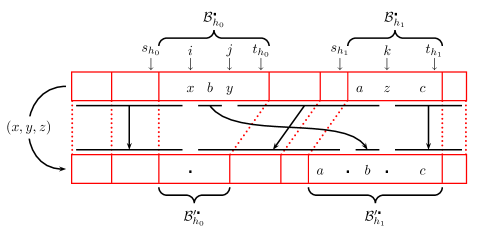
(b)

Figure 7: Effects of a 3DT-step $\underrightarrow{\;(d,e,f)\;}$ on an $l$-block-decomposition if (a) $(d,e,f)$ is an internal triple, or (b) there exists a variable $A=[(a,b,c),(x,y,z)]$ such that $(d,e,f)=(x,y,z)$. Both figures are in fact derived from Figure 3 in the context of an $l$-block-decomposition.

Consider a block $B$ in a valid context $(I,\mathcal{B})$ (there exists $h\in\left\llbracket 1\,;\,l\right\rrbracket$ such that $B=\mathcal{B}_{h}$), and $(d,e,f)$ a triple of $I$ such that $(I,\mathcal{B})\raisebox{5.0pt}{\scriptsize$\underrightarrow{\;(d,e,f)\;}$}(I^{\prime},\mathcal{B}^{\prime})$ (we write $B^{\prime}=\mathcal{B}^{\prime}_{h}$). Then, following Property 12, four cases are possible:

• $h\notin\{block_{I,\mathcal{B}}(d),block_{I,\mathcal{B}}(e),block_{I,\mathcal{B}}(f)\}$, hence $B^{\prime}=B$, since, by Property 12, the relative order of the elements of $B$ remains unchanged after the 3DT-step $\underrightarrow{\;(d,e,f)\;}$.

• $(d,e,f)$ is an internal triple of $B$. We write

  

• $\exists A=[(a,b,c),(x,y,z)]$ such that $h=source(A)$ and $(d,e,f)=(x,y,z)$ ($A$ is an output of $B$), see Figure 8 (left). We write

  

• $\exists A=[(a,b,c),(x,y,z)]$ such that $h=target(A)$ and $(d,e,f)=(x,y,z)$ ($A$ is an input of $B$), see Figure 8 (right). We write

  

The graph obtained from a block $B$ by following exhaustively the possible arcs as defined above (always assuming this block is in a valid context) is called the behavior graph of $B$.

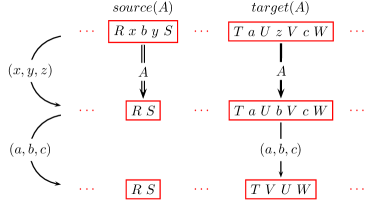
Figure 8: The activation of a variable $A=[(a,b,c),(x,y,z)]$ is written with a double arc in the behavior graph of the source block of $A$ and with a thick arc in the behavior graph of its target block. It can be followed by the 3DT-step $\underrightarrow{\;(a,b,c)\;}$, impacting only the target block of $A$. Dot symbols ($\centerdot$) are omitted. We denote by $R,S,T,U,V,W$ some factors of the source and target blocks of $A$: the consequence of activating $A$ is to allow $U$ and $V$ to be swapped in $target(A)$.

3.2 Basic Blocks

We now define four basic blocks: $\mathsf{copy}$, $\mathsf{and}$, $\mathsf{or}$, and $\mathsf{var}$. They are studied independently in this section, before being assembled in Section 3.3. Each of these blocks is defined by a word and a set of triples. We distinguish internal triples, for which all three elements appear in a single block, from external triples, which are part of an input/output variable, and for which only one or two elements appear in the block. Note that each external triple is part of an input (resp. output) variable, which itself must be an output (resp. input) of another block, the other block containing the remaining elements of the triple.

We then draw the behavior graph of each of these blocks (Figures 9 to 12): in each case, we assume that the block is in a valid context, and follow exhaustively the 3DT-steps that can be applied on it. We then give another graph (Figures 13a to  13d), obtained from the behavior graph by contracting all arcs corresponding to 3DT-steps using internal triples, i.e. we assimilate every pair of nodes linked by such an arc. Hence, only the arcs corresponding to the activation of an input/output variable remain. From this second figure, we derive a property describing the behavior of the block, in terms of activating input and output variables (always provided this block is in a valid context). It must be kept in mind that for any variable, it is the state of the source block which determines whether it can be activated, whereas the activation itself affects mostly the target block.

3.2.1 The block $\mathsf{copy}$

This block aims at duplicating a variable: any of the two output variables can only be activated after the input variable has been activated.

Input variable: $A=[(a,b,c),(x,y,z)]$.

Output variables: $A_{1}=[(a_{1},b_{1},c_{1}),(x_{1},y_{1},z_{1})]$ and $A_{2}=[(a_{2},b_{2},c_{2}),(x_{2},y_{2},z_{2})]$.

Internal triple: $(d,e,f)$.

Definition:

$$\text{\fcolorbox{red}{white}{$ [A_1,A_2]=\blockFont{copy}(A)$}}\quad=\quad\text{\fcolorbox{red}{white}{$ a\ y_1\ e\ z\ d\ y_2\ x_1\ b_1\ c\ x_2\ b_2\ f$}}$$

Property 14.

In a block $[A_{1},A_{2}]=\mathsf{copy}(A)$ in a valid context, the possible orders in which $A$, $A_{1}$ and $A_{2}$ can be activated are $(A,A_{1},A_{2})$ and $(A,A_{2},A_{1})$.

Proof.

See Figures 9 and 13a. ∎

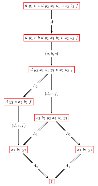
Figure 9: Behavior graph of the block $[A_{1},A_{2}]=\mathsf{copy}(A)$. A thick (resp. double) arc corresponds to the 3DT-step $\underrightarrow{\;(x,y,z)\;}$ for an input (resp. output) variable $[(a,b,c),(x,y,z)]$.

3.2.2 The block $\mathsf{and}$

This block aims at simulating a conjunction: the output variable can only be activated after both input variables have been activated.

Input variables: $A_{1}=[(a_{1},b_{1},c_{1}),(x_{1},y_{1},z_{1})]$ and $A_{2}=[(a_{2},b_{2},c_{2}),(x_{2},y_{2},z_{2})]$.

Output variable: $A=[(a,b,c),(x,y,z)]$.

Internal triple: $(d,e,f)$.

Definition:

$$\text{\fcolorbox{red}{white}{$ A=\blockFont{and}(A_1,A_2)$}}\quad=\quad\text{\fcolorbox{red}{white}{$ a_1\ e\ z_1\ a_2\ c_1\ z_2\ d\ y\ c_2\ x\ b\ f$}}$$

Property 15.

In a block $A=\mathsf{and}(A_{1},A_{2})$ in a valid context, the possible orders in which $A$, $A_{1}$ and $A_{2}$ can be activated are $(A_{1},A_{2},A)$ and $(A_{2},A_{1},A)$.

Proof.

See Figures 10 and 13b. ∎

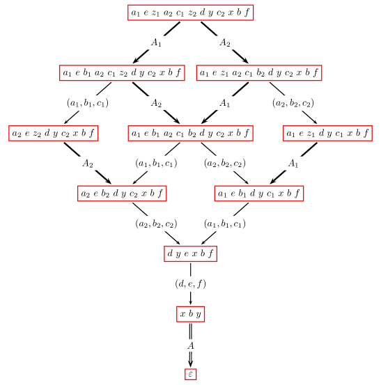
Figure 10: Behavior graph of the block $A=\mathsf{and}(A_{1},A_{2})$.

3.2.3 The block $\mathsf{or}$

This block aims at simulating a disjunction: the output variable can be activated as soon as any of the two input variables is activated.

Input variables: $A_{1}=[(a_{1},b_{1},c_{1}),(x_{1},y_{1},z_{1})]$ and $A_{2}=[(a_{2},b_{2},c_{2}),(x_{2},y_{2},z_{2})]$.

Output variable: $A=[(a,b,c),(x,y,z)]$.

Internal triples: $(a^{\prime},b^{\prime},c^{\prime})$ and $(d,e,f)$.

Definition:

$$\text{\fcolorbox{red}{white}{$ A=\blockFont{or}(A_1,A_2)$}}\quad=\quad\text{\fcolorbox{red}{white}{$ a_1\ b'\ z_1\ a_2\ d\ y\ a'\ x\ b\ f\ z_2\ c_1\ e\ c'\ c_2$}}$$

Property 16.

In a block $A=\mathsf{or}(A_{1},A_{2})$ in a valid context, the possible orders in which $A$, $A_{1}$ and $A_{2}$ can be activated are $(A_{1},A,A_{2})$, $(A_{2},A,A_{1})$, $(A_{1},A_{2},A)$ and $(A_{2},A_{1},A)$.

Proof.

See Figures 11 and 13c. ∎

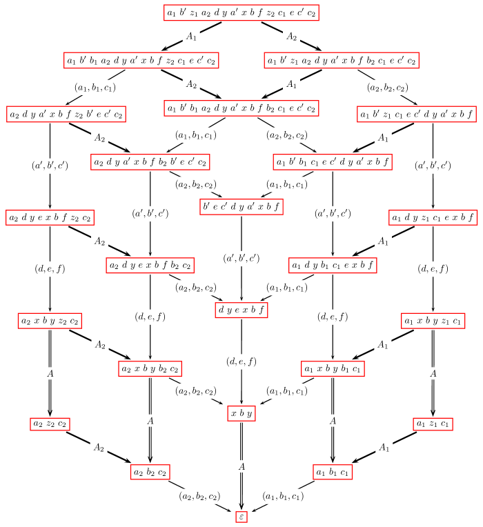
Figure 11: Behavior graph of the block $A=\mathsf{or}(A_{1},A_{2})$.

3.2.4 The block $\mathsf{var}$

This block aims at simulating a boolean variable: in a first stage, only one of the two output variables can be activated. The other needs the activation of the input variable to be activated.

Input variable: $A=[(a,b,c),(x,y,z)]$.

Output variables: $A_{1}=[(a_{1},b_{1},c_{1}),(x_{1},y_{1},z_{1})]$, $A_{2}=[(a_{2},b_{2},c_{2}),(x_{2},y_{2},z_{2})]$.

Internal triples: $(d_{1},e_{1},f_{1})$, $(d_{2},e_{2},f_{2})$ and $(a^{\prime},b^{\prime},c^{\prime})$.

Definition:

$$\text{\fcolorbox{red}{white}{$ [A_1,A_2]=\blockFont{var}(A\zz)$}}\quad=\quad\text{\fcolorbox{red}{white}{$ d_1\ y_1\ a\zz\ d_2\ y_2\ e_1\ a'\ e_2\ x_1\ b_1\ f_1\ c'\ z\zz\ b'\ c\zz\ x_2\ b_2\ f_2$}}$$

Property 17.

In a block $[A_{1},A_{2}]=\mathsf{var}(A)$ in a valid context, the possible orders in which $A$, $A_{1}$ and $A_{2}$ can be activated are $(A_{1},A,A_{2})$, $(A_{2},A,A_{1})$, $(A,A_{1},A_{2})$ and $(A,A_{2},A_{1})$.

Proof.

See Figures 12 and 13d. ∎

With such a block, if $A$ is not activated first, one needs to make a choice between activating $A_{1}$ or $A_{2}$. Once $A$ is activated, however, all remaining output variables are activable.

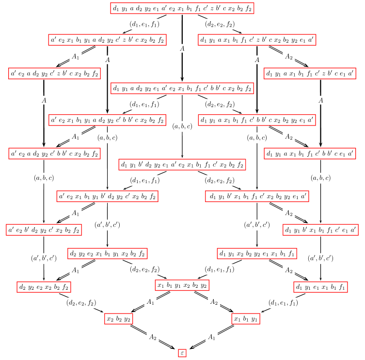
Figure 12: Behavior graph of the block $[A_{1},A_{2}]=\mathsf{var}(A)$.

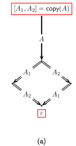
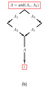
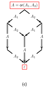
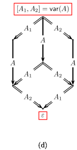
Figure 13: Abstract representations of the blocks $\mathsf{copy}$, $\mathsf{and}$, $\mathsf{or}$, and $\mathsf{var}$, obtained from each behavior graph (Figures 9, 10, 11 and 12) by contracting arcs corresponding to internal triples, and keeping only the arcs corresponding to variables. We see, for each block, which output variables are activable, depending on which variables have been activated.

3.2.5 Assembling the blocks $\mathsf{copy}$, $\mathsf{and}$, $\mathsf{or}$, $\mathsf{var}$.

Definition 14 (Assembling of basic blocks).

An assembling of basic blocks $(I,\mathcal{B})$ is composed of a 3DT-instance $I$ and an $l$-block-decomposition $\mathcal{B}$ obtained by the following process:

• Create a set of variables $\mathcal{A}$.

• Define $I=\left<\Sigma,T,\psi\right>$ by its word representation, as a concatenation of $l$ factors $\mathcal{B}^{\raisebox{0.70004pt}{$\centerdot$}}_{1}\ \mathcal{B}^{\raisebox{0.70004pt}{$\centerdot$}}_{2}\ \ldots\ \mathcal{B}^{\raisebox{0.70004pt}{$\centerdot$}}_{l}$ and a set of triples $T$, where each $\mathcal{B}^{\raisebox{0.70004pt}{$\centerdot$}}_{h}$ is one of the blocks $[A_{1},A_{2}]=\mathsf{copy}(A)$, $A=\mathsf{and}(A_{1},A_{2})$, ${A=\mathsf{or}(A_{1},A_{2})}$ or $[A_{1},A_{2}]=\mathsf{var}(A)$, with $A_{1},A_{2},A\in\mathcal{A}$ (such that each $X\in\mathcal{A}$ appears in the input of exactly one block, and in the output of exactly one other block); and where $T$ is the union of the set of internal triples needed in each block, and the set of external triples defined by the variables of $\mathcal{A}$.

Example 2.

We create a 3DT-instance $I$ with a 2-block-decomposition $\mathcal{B}$ such that $(I,\mathcal{B})$ is an assembling of basic blocks, defined as follows:

• $I$ uses three variables, $\mathcal{A}=\{X_{1},X_{2},Y\}$

• the word representation of $I$ is the concatenation of $[X_{1},X_{2}]=\mathsf{var}(Y)$ and $Y=\mathsf{or}(X_{1},X_{2})$

With $X_{1}=[(a_{1},b_{1},c_{1}),(x_{1},y_{1},z_{1})]$, $X_{2}=[(a_{2},b_{2},c_{2}),(x_{2},y_{2},z_{2})]$, $Y=[(a,b,c),(x,y,z)]$, and the internal triples $(d_{1},e_{1},f_{1}),(d_{2},e_{2},f_{2}),(a^{\prime},b^{\prime},c^{\prime})$ for the block $\mathsf{var}$, and $(a^{\prime\prime},b^{\prime\prime},c^{\prime\prime}),(d,e,f)$ for the block $\mathsf{or}$, the word representation of $I$ is the following (note that its 2-block-decomposition is $(0,18)$):

$$I=d_{1}\ y_{1}\ a\ d_{2}\ y_{2}\ e_{1}\ a^{\prime}\ e_{2}\ x_{1}\ b_{1}\ f_{1}\ c^{\prime}\ z\ b^{\prime}\ c\ x_{2}\ b_{2}\ f_{2}\quad a_{1}\ b^{\prime\prime}\ z_{1}\ a_{2}\ d\ y\ a^{\prime\prime}\ x\ b\ f\ z_{2}\ c_{1}\ e\ c^{\prime\prime}\ c_{2}$$

Indeed, a possible sequence of 3DT-steps leading from $I$ to $\varepsilon$ is given in Figure 14, hence $I$ is 3DT-collapsible.

$$I =|\ \text{\boldmath$d_{1}$}\ \underline{\vphantom{f_{f_{f}}}y_{1}\ a\ d_{2}\ y_{2}}\ \text{\boldmath$e_{1}$}\ \underline{\vphantom{f_{f_{f}}}\mbox{$a^{\prime}\ e_{2}\ x_{1}\ b_{1}$}}\ \text{\boldmath$f_{1}$}\ c^{\prime}\ z\ b^{\prime}\ c\ x_{2}\ b_{2}\ f_{2}\ |\ a_{1}\ b^{\prime\prime}\ z_{1}\ a_{2}\ d\ y\ a^{\prime\prime}\ x\ b\ f\ z_{2}\ c_{1}\ e\ c^{\prime\prime}\ c_{2}\ |$$

$$\downarrow (d_{1},e_{1},f_{1}) \mathcal{B}_{1}$$    Internal triple of

$$I_{10} =|\ a^{\prime}\ e_{2}\ \text{\boldmath$x_{1}$}\ \underline{\vphantom{f_{f_{f}}}b_{1}}\ \text{\boldmath$y_{1}$}\ \underline{\vphantom{f_{f_{f}}}a\ d_{2}\ y_{2}\ c^{\prime}\ z\ b^{\prime}\ c\ x_{2}\ b_{2}\ f_{2}\ |\ a_{1}\ b^{\prime\prime}}\ \text{\boldmath$z_{1}$}\ a_{2}\ d\ y\ a^{\prime\prime}\ x\ b\ f\ z_{2}\ c_{1}\ e\ c^{\prime\prime}\ c_{2}\ |$$

$$\downarrow (x_{1},y_{1},z_{1}) X_{1}$$    Activation of

$$I_{9} =|\ a^{\prime}\ e_{2}\ a\ d_{2}\ y_{2}\ c^{\prime}\ z\ b^{\prime}\ c\ x_{2}\ b_{2}\ f_{2}\ |\ \text{\boldmath$a_{1}$}\ \underline{\vphantom{f_{f_{f}}}b^{\prime\prime}}\ \text{\boldmath$b_{1}$}\ \underline{\vphantom{f_{f_{f}}}a_{2}\ d\ y\ a^{\prime\prime}\ x\ b\ f\ z_{2}}\ \text{\boldmath$c_{1}$}\ e\ c^{\prime\prime}\ c_{2}\ |$$

$$\downarrow (a_{1},b_{1},c_{1}) \mathcal{B}_{2}$$    Internal triple of

$$I_{8} =|\ a^{\prime}\ e_{2}\ a\ d_{2}\ y_{2}\ c^{\prime}\ z\ b^{\prime}\ c\ x_{2}\ b_{2}\ f_{2}\ |\ a_{2}\ d\ y\ \text{\boldmath$a^{\prime\prime}$}\ \underline{\vphantom{f_{f_{f}}}x\ b\ f\ z_{2}}\ \text{\boldmath$b^{\prime\prime}$}\ \underline{\vphantom{f_{f_{f}}}e}\ \text{\boldmath$c^{\prime\prime}$}\ c_{2}\ |$$

$$\downarrow (a^{\prime\prime},b^{\prime\prime},c^{\prime\prime}) \mathcal{B}_{2}$$    Internal triple of

$$I_{7} =|\ a^{\prime}\ e_{2}\ a\ d_{2}\ y_{2}\ c^{\prime}\ z\ b^{\prime}\ c\ x_{2}\ b_{2}\ f_{2}\ |\ a_{2}\ \text{\boldmath$d$}\ \underline{\vphantom{f_{f_{f}}}y}\ \text{\boldmath$e$}\ \underline{\vphantom{f_{f_{f}}}x\ b}\ \text{\boldmath$f$}\ z_{2}\ c_{2}\ |$$

$$\downarrow (d,e,f) \mathcal{B}_{2}$$    Internal triple of

$$I_{6} =|\ a^{\prime}\ e_{2}\ a\ d_{2}\ y_{2}\ c^{\prime}\ \text{\boldmath$z$}\ \underline{\vphantom{f_{f_{f}}}b^{\prime}\ c\ x_{2}\ b_{2}\ f_{2}\ |\ a_{2}}\ \text{\boldmath$x$}\ \underline{\vphantom{f_{f_{f}}}b}\ \text{\boldmath$y$}\ z_{2}\ c_{2}\ |$$

$$\downarrow (x,y,z) Y$$    Activation of

$$I_{5} =|\ a^{\prime}\ e_{2}\ \text{\boldmath$a$}\ \underline{\vphantom{f_{f_{f}}}d_{2}\ y_{2}\ c^{\prime}}\ \text{\boldmath$b$}\ \underline{\vphantom{f_{f_{f}}}b^{\prime}}\ \text{\boldmath$c$}\ x_{2}\ b_{2}\ f_{2}\ |\ a_{2}\ z_{2}\ c_{2}\ |$$

$$\downarrow (a,b,c) \mathcal{B}_{1}$$    Internal triple of

$$I_{4} =|\ \text{\boldmath$a^{\prime}$}\ \underline{\vphantom{f_{f_{f}}}e_{2}}\ \text{\boldmath$b^{\prime}$}\ \underline{\vphantom{f_{f_{f}}}d_{2}\ y_{2}}\ \text{\boldmath$c^{\prime}$}\ x_{2}\ b_{2}\ f_{2}\ |\ a_{2}\ z_{2}\ c_{2}\ |$$

$$\downarrow (a^{\prime},b^{\prime},c^{\prime}) \mathcal{B}_{1}$$    Internal triple of

$$I_{3} =|\ \text{\boldmath$d_{2}$}\ \underline{\vphantom{f_{f_{f}}}y_{2}}\ \text{\boldmath$e_{2}$}\ \underline{\vphantom{f_{f_{f}}}x_{2}\ b_{2}}\ \text{\boldmath$f_{2}$}\ |\ a_{2}\ z_{2}\ c_{2}\ |$$

$$\downarrow (d_{2},e_{2},f_{2}) \mathcal{B}_{1}$$    Internal triple of

$$I_{2} =|\ \text{\boldmath$x_{2}$}\ \underline{\vphantom{f_{f_{f}}}b_{2}}\ \text{\boldmath$y_{2}$}\underline{\vphantom{f_{f_{f}}}\ |\ a_{2}}\ \text{\boldmath$z_{2}$}\ c_{2}\ |$$

$$\downarrow (x_{2},y_{2},z_{2}) X_{2}$$    Activation of

$$I_{1} =|\ \varepsilon\ |\ \text{\boldmath$a_{2}\ b_{2}\ c_{2}$}\ |$$

$$\downarrow (a_{2},b_{2},c_{2}) \mathcal{B}_{2}$$    Internal triple of

$$I_{0} =|\ \varepsilon\ |\ \varepsilon\ |=\varepsilon$$

Figure 14: 3DT-collapsibility of the assembling of basic blocks ${[X_{1},X_{2}]=\mathsf{var}(Y)}$ and ${Y=\mathsf{or}(X_{1},X_{2})}$. For each 3DT-step, the three elements that are deleted from the alphabet are in bold, the elements that are swapped by the corresponding transposition are underlined. Vertical bars give the limits of the blocks in the 2-block-decomposition, and dot symbols are omitted.

Lemma 18.

Let $I^{\prime}$ be a 3DT-instance with an $l$-block-decomposition $\mathcal{B}^{\prime}$, such that $(I^{\prime},\mathcal{B}^{\prime})$ is obtained from an assembling of basic blocks $(I,\mathcal{B})$ after any number of 3DT-steps, i.e. there exist $k\geq 0$ triples $(d_{i},e_{i},f_{i})$, $i\in\left\llbracket 1\,;\,k\right\rrbracket$, such that $(I,\mathcal{B})\raisebox{5.0pt}{\scriptsize$\underrightarrow{\;(d_{1},e_{1},f_{1})\;}$}\cdots\raisebox{5.0pt}{\scriptsize$\underrightarrow{\;(d_{k},e_{k},f_{k})\;}$}(I^{\prime},\mathcal{B}^{\prime})$.

Then $(I^{\prime},\mathcal{B}^{\prime})$ is a valid context. Moreover, if the set of variables of $(I^{\prime},\mathcal{B}^{\prime})$ is empty, then $I^{\prime}$ is 3DT-collapsible.

Proof.

Write $\mathcal{A}$ the set of variables used to define $(I,\mathcal{B})$. We write $I=\left<\Sigma,T,\psi\right>$ and $I^{\prime}=\left<\Sigma^{\prime},T^{\prime},\psi^{\prime}\right>$. We prove that $(I^{\prime},\mathcal{B}^{\prime})$ is a valid context by induction on $k$ (the number of 3DT-steps between $(I,\mathcal{B})$ and $(I^{\prime},\mathcal{B}^{\prime})$). We also prove that for each $h\in\left\llbracket 1\,;\,l\right\rrbracket$, $\mathcal{B}^{\prime}_{h}$ appears as a node in the behavior graph of $\mathcal{B}_{h}$.

Suppose first that $k=0$. We show that the set of external triples of $(I,\mathcal{B})=(I^{\prime},\mathcal{B}^{\prime})$ can be partitioned into valid variables, namely into $\mathcal{A}$. Indeed, from the definition of each block, for each $\sigma\in\Sigma$, $\sigma$ is either part of an internal triple, or appears in a variable $A\in\mathcal{A}$. Conversely, for each $A=[(a,b,c),(x,y,z)]\in\mathcal{A}$, $b$, $x$ and $y$ appear in the block having $A$ for output, and $a$, $c$ and $z$ appear in the block having $A$ for input. Hence $(a,b,c)$ and $(x,y,z)$ are indeed two external triples of $(I,\mathcal{B})$. Hence each variable satisfies conditions (i) and (ii) of Definition 12. Conditions (iii) and (iv) can be checked in the definition of each block: we have, for each output variable, $y\prec x$, and for each input variable, $a\prec z\prec c$. Finally, each $\mathcal{B}_{h}$ appears in its own behavior graph.

Suppose now that $(I^{\prime},\mathcal{B}^{\prime})$ is obtained from $(I,\mathcal{B})$ after $k$ 3DT-steps, $k>0$. Then there exists a 3DT-instance with an $l$-block-decomposition $(I^{\prime\prime},\mathcal{B}^{\prime\prime})$ such that:

$$(I,\mathcal{B})\raisebox{5.0pt}{\scriptsize$\underrightarrow{\;(d_{1},e_{1},f_{1})\;}$}\cdots\raisebox{5.0pt}{\scriptsize$\underrightarrow{\;(d_{k-1},e_{k-1},f_{k-1})\;}$}(I^{\prime\prime},\mathcal{B}^{\prime\prime})\raisebox{5.0pt}{\scriptsize$\underrightarrow{\;(d_{k},e_{k},f_{k})\;}$}(I^{\prime},\mathcal{B}^{\prime}).$$

Consider $h\in\left\llbracket 1\,;\,l\right\rrbracket$. By induction hypothesis, since $\mathcal{B}^{\prime\prime}_{h}$ is in a valid context $(I^{\prime\prime},\mathcal{B}^{\prime\prime})$, then, depending on $(d_{k},e_{k},f_{k})$, either $\mathcal{B}^{\prime}_{h}=\mathcal{B}^{\prime\prime}_{h}$, either there is an arc from $\mathcal{B}^{\prime\prime}_{h}$ to $\mathcal{B}^{\prime}_{h}$ in the behavior graph. Hence $\mathcal{B}^{\prime}_{h}$ is indeed a node in this graph. By Property 13, we know that the set of external triples of $(I^{\prime},\mathcal{B}^{\prime})$ can be partitioned into variables satisfying conditions (i) and (ii) of Definition 12. Hence we need to prove that each variable satisfies conditions (iii) and (iv): we verify, for each node of each behavior graph, that $x\prec y\Rightarrow x\triangleleft b\triangleleft y$ (resp. $a\prec z\prec c$) for each output (resp. input) variable $A=[(a,b,c),(x,y,z)]$ of the block. This achieves the induction proof.

We finally need to consider the case where the set of variables of $(I^{\prime},\mathcal{B}^{\prime})$ is empty. Then for each $h\in\left\llbracket 1\,;\,l\right\rrbracket$ we either have $\mathcal{B}^{\prime}_{h}=\varepsilon$, or $\mathcal{B}^{\prime}_{h}=a_{h}\ b_{h}\ c_{h}$ for some internal triple $(a_{h},b_{h},c_{h})$ (in the case where $\mathcal{B}_{h}$ is a block $\mathsf{or}$). Then $(I^{\prime},\mathcal{B}^{\prime})$ is indeed 3DT-collapsible: simply follow in any order the 3DT-step $\underrightarrow{\;(a_{h},b_{h},c_{h})\;}$ for each remaining triple $(a_{h},b_{h},c_{h})$. ∎

3.3 Construction

Let $\phi$ be a boolean formula, over the boolean variables $x_{1},\ldots,x_{m}$, given in conjunctive normal form: $\phi=C_{1}\wedge C_{2}\wedge\ldots\wedge C_{\gamma}$. Each clause $C_{c}$ ($c\in\left\llbracket 1\,;\,\gamma\right\rrbracket$) is the disjunction of a number of literals, $x_{i}$ or $\neg x_{i}$, $i\in\left\llbracket 1\,;\,m\right\rrbracket$. We write $q_{i}$ (resp. $\bar{q}_{i}$) the number of occurrences of the literal $x_{i}$ (resp. $\neg x_{i}$) in $\phi$, $i\in\left\llbracket 1\,;\,m\right\rrbracket$. We also write $k(C_{c})$ the number of literals appearing in the clause $C_{c}$, $c\in\left\llbracket 1\,;\,\gamma\right\rrbracket$. We can assume that $\gamma\geq 2$, that for each $c\in\left\llbracket 1\,;\,\gamma\right\rrbracket$, we have $k(C_{c})\geq 2$, and that for each $i\in\left\llbracket 1\,;\,m\right\rrbracket$, $q_{i}\geq 2$ and $\bar{q}_{i}\geq 2$. (Otherwise, we can always add clauses of the form $(x_{i}\vee\neg x_{i})$ to $\phi$, or duplicate the literals appearing in the clauses $C_{c}$ such that $k(C_{c})=1$.) In order to distinguish variables of an $l$-block-decomposition from $x_{1},\ldots,x_{m}$, we always use the term boolean variable for the latter.

The 3DT-instance $I_{\phi}$ is defined as an assembling of basic blocks: we first define a set of variables, then we list the blocks of which the word representation of $I_{\phi}$ is the concatenation. It is necessary that each variable is part of the input (resp. the output) of exactly one block. Note that the relative order of the blocks is of no importance. We simply try, for readability reasons, to ensure that the source of a variable appears before its target, whenever possible. We say that a variable represents a term, i.e. a literal, clause or formula, if it can be activated only if this term is true (for some fixed assignment of the boolean variables), or if $\phi$ is satisfied by this assignment. We also say that a block defines a variable if it is its source block.

The construction of $I_{\phi}$ is done as follows (see Figure 15 for an example):

• Create a set of variables:

  • For each $i\in\left\llbracket 1\,;\,m\right\rrbracket$, create $q_{i}+1$ variables representing $x_{i}$: $X_{i}$ and $X_{i}^{j}$, $j\in\left\llbracket 1\,;\,q_{i}\right\rrbracket$, and $\bar{q}_{i}+1$ variables representing $\neg x_{i}$: $\bar{X}_{i}$ and $\bar{X}_{i}^{j}$, $j\in\left\llbracket 1\,;\,\bar{q}_{i}\right\rrbracket$.

  • For each $c\in\left\llbracket 1\,;\,\gamma\right\rrbracket$, create a variable $\Gamma_{c}$ representing the clause $C_{c}$.

  • Create $m+1$ variables, $A_{\phi}$ and $A_{\phi}^{i}$, $i\in\left\llbracket 1\,;\,m\right\rrbracket$, representing the formula $\phi$. We will show that $A_{\phi}$ has a key role in the construction: it can be activated only if $\phi$ is satisfiable, and, once activated, it allows every remaining variable to be activated.

  • We also use a number of intermediate variables, with names $U$, $\bar{U}$, $V$, $W$ and $Y$.

• Start with an empty 3DT-instance $\varepsilon$, and add blocks successively:

  • For each $i\in\left\llbracket 1\,;\,m\right\rrbracket$, add the following $q_{i}+\bar{q}_{i}-1$ blocks defining the variables $X_{i}$, $X_{i}^{j}$ ($j\in\left\llbracket 1\,;\,q_{i}\right\rrbracket$), and $\bar{X}_{i}$, $\bar{X}_{i}^{j}$ ($j\in\left\llbracket 1\,;\,\bar{q}_{i}\right\rrbracket$):

    $$[X_{i},\bar{X}_{i}]=\mathsf{var}(A_{\phi}^{i})$$

    $$[X_{i}^{1},U_{i}^{2}] =\mathsf{copy}(X_{i}) [\bar{X}_{i}^{1},\bar{U}_{i}^{2}] =\mathsf{copy}(\bar{X}_{i})$$

    $$[X_{i}^{2},U_{i}^{3}] =\mathsf{copy}(U_{i}^{2}) [\bar{X}_{i}^{2},\bar{U}_{i}^{3}] =\mathsf{copy}(\bar{U}_{i}^{2})$$

    $$\>\ \vdots \>\ \vdots {*}$$ ()

    $$[X_{i}^{q_{i}-2},U_{i}^{q_{i}-1}] =\mathsf{copy}(U_{i}^{q_{i}-2}) \>\ \vdots$$

    $$[X_{i}^{q_{i}-1},X_{i}^{q_{i}}] =\mathsf{copy}(U_{i}^{q_{i}-1}) [\bar{X}_{i}^{\bar{q}_{i}-2},\bar{U}_{i}^{\bar{q}_{i}-1}] =\mathsf{copy}(\bar{U}_{i}^{\bar{q}_{i}-2})$$

    $$[\bar{X}_{i}^{\bar{q}_{i}-1},\bar{X}_{i}^{\bar{q}_{i}}] =\mathsf{copy}(\bar{U}_{i}^{\bar{q}_{i}-1})$$

  • For each $c\in\left\llbracket 1\,;\,\gamma\right\rrbracket$, let $C_{c}=\lambda_{1}\vee\lambda_{2}\vee\ldots\vee\lambda_{k}$, with $k=k(C_{c})$. Let each $\lambda_{p}$, $p\in\left\llbracket 1\,;\,k\right\rrbracket$, be the $j$-th occurrence of a literal $x_{i}$ or $\neg x_{i}$, for some $i\in\left\llbracket 1\,;\,m\right\rrbracket$ and $j\in\left\llbracket 1\,;\,q_{i}\right\rrbracket$ (resp. $j\in\left\llbracket 1\,;\,\bar{q}_{i}\right\rrbracket$). We respectively write $L_{p}=X_{i}^{j}$ or $L_{p}=\bar{X}_{i}^{j}$. We add the following $k-1$ blocks defining $\Gamma_{c}$:

    $$V_{c}^{2} =\mathsf{or}(L_{1},L_{2})$$

    $$V_{c}^{3} =\mathsf{or}(V_{c}^{2},L_{3})$$

    $$\ \>\vdots {*}{*}$$ ()

    $$V_{c}^{k-1} =\mathsf{or}(V_{c}^{k-2},L_{k-1})$$

    $$\Gamma_{c} =\mathsf{or}(V_{c}^{k-1},L_{k})$$

  • Since $\phi=C_{1}\wedge C_{2}\wedge\ldots\wedge C_{\gamma}$, the formula variable $A_{\phi}$ is defined by the following $\gamma-1$ blocks:

    $$W_{2} =\mathsf{and}(\Gamma_{1},\Gamma_{2})$$

    $$W_{3} =\mathsf{and}(W_{2},\Gamma_{3})$$

    $$\ \>\vdots {*}{*}{*}$$ ()

    $$W_{\gamma-1} =\mathsf{and}(W_{\gamma-2},\Gamma_{\gamma-1})$$

    $$A_{\phi} =\mathsf{and}(W_{\gamma-1},\Gamma_{l})$$

  • The $m$ copies $A^{1}_{\phi},\ldots,A^{m}_{\phi}$ of $A_{\phi}$ are defined with the following $m-1$ blocks:

    $$[A_{\phi}^{1},Y_{2}] =\mathsf{copy}(A_{\phi})$$

    $$[A_{\phi}^{2},Y_{3}] =\mathsf{copy}(Y_{2})$$

    $$\ \>\vdots {*}{*}{*}{*}$$ ()

    $$[A_{\phi}^{m-2},Y_{m-1}] =\mathsf{copy}(Y_{m-2})$$

    $$[A_{\phi}^{m-1},A_{\phi}^{m}] =\mathsf{copy}(Y_{m-1})$$

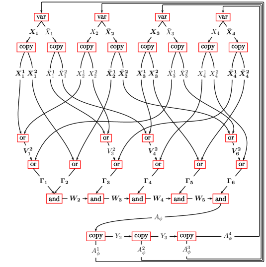
Figure 15: Schematic diagram of the blocks defining $I_{\phi}$ for $\phi={(x_{1}\vee x_{2}\vee\neg x_{3})}\wedge{(x_{1}\vee\neg x_{2})}\wedge{(\neg x_{1}\vee x_{2}\vee\neg x_{4})}\wedge{(\neg x_{1}\vee x_{3}\vee x_{4})}\wedge{(x_{3}\vee\neg x_{4})}\wedge{(\neg x_{2}\vee\neg x_{3}\vee x_{4})}$. For each variable, we draw an arc between its source and target block. Note that $\phi$ is satisfiable (e.g. with the assignment $x_{1}=x_{3}=true$ and $x_{2}=x_{4}=false$). A set of variables that can be activated before $A_{\phi}$ is in bold, they correspond to the terms being true in $\phi$ for the assignment $x_{1}=x_{3}=true$ and $x_{2}=x_{4}=false$.

3.4 Main Result

Theorem 19.

Let $\phi$ be a boolean formula, and $I_{\phi}$ the 3DT-instance defined in Section 3.3. The construction of $I_{\phi}$ is polynomial in the size of $\phi$, and $\phi$ is satisfiable iff $I_{\phi}$ is 3DT-collapsible.

Proof.

The polynomial time complexity of the construction of $I_{\phi}$ is trivial. We use the same notations as in the construction, with $\mathcal{B}$ the block decomposition of $I_{\phi}$. One can easily check, in (${*}$ ‣ – ‣ • ‣ 3.3), (${*}{*}$ ‣ – ‣ • ‣ 3.3), (${*}{*}{*}$ ‣ – ‣ • ‣ 3.3) and (${*}{*}{*}{*}$ ‣ – ‣ • ‣ 3.3), each variable has exactly one source block and one target block. Then, by Lemma 18, we know that $(I_{\phi},\mathcal{B})$ is a valid context, and remains so after any number of 3DT-steps, hence properties 14, 15, 16 and 17 are satisfied by respectively each block $\mathsf{copy}$, $\mathsf{and}$, $\mathsf{or}$ and $\mathsf{var}$ of $I_{\phi}$.

$\Rightarrow$ Assume first that $\phi$ is satisfiable. Consider a truth assignment satisfying $\phi$: let $P$ be the set of indices $i\in\left\llbracket 1\,;\,m\right\rrbracket$ such that $x_{i}$ is assigned to true. Starting from $I_{\phi}$, we can follow a path of 3DT-steps that activates all the variables of $I_{\phi}$ in the following order:

• For $i\in\left\llbracket 1\,;\,m\right\rrbracket$, if $i\in P$, activate $X_{i}$ in the corresponding block $\mathsf{var}$ in (${*}$ ‣ – ‣ • ‣ 3.3). Then, with the blocks $\mathsf{copy}$, activate successively all intermediate variables $U_{i}^{j}$ for $j=2$ to $q_{i}-1$, and variables $X^{j}_{i}$ for $j\in\left\llbracket 1\,;\,q_{i}\right\rrbracket$.

  Otherwise, if $i\notin P$, activate $\bar{X}_{i}$, all intermediate variables $\bar{U}_{i}^{j}$ for $j=2$ to $\bar{q}_{i}-1$, and the variables $\bar{X}^{j}_{i}$ for $j\in\left\llbracket 1\,;\,\bar{q}_{i}\right\rrbracket$

• For each $c\in\left\llbracket 1\,;\,\gamma\right\rrbracket$, let $C_{c}=\lambda_{1}\vee\lambda_{2}\vee\ldots\vee\lambda_{k}$, with $k=k(C_{c})$. Since $C_{c}$ is true with the selected truth assignment, at least one literal $\lambda_{p_{0}}$, ${p_{0}}\in\left\llbracket 1\,;\,k\right\rrbracket$, is true. If $\lambda_{p_{0}}$ is the $j$-th occurrence of a literal $x_{i}$ or $\neg x_{i}$, then the corresponding variable $L_{p_{0}}$ ($L_{p_{0}}=X_{i}^{j}$ or $L_{p_{0}}=\bar{X}_{i}^{j}$) has been activated previously. Using the blocks $\mathsf{or}$ in (${*}{*}$ ‣ – ‣ • ‣ 3.3), we activate successively each intermediate variable $V_{c}^{p}$ for $p={p_{0}}$ to $p=k-1$, and finally we activate the variable $\Gamma_{c}$.

• Since all variables $\Gamma_{c}$, $c\in\left\llbracket 1\,;\,\gamma\right\rrbracket$, have been activated, using the blocks $\mathsf{and}$ in (${*}{*}{*}$ ‣ – ‣ • ‣ 3.3), we activate each intermediate variable $W_{c}$ for $c=2$ to $c=\gamma-1$, and the formula variable $A_{\phi}$.

• With the blocks $\mathsf{copy}$ in (${*}{*}{*}{*}$ ‣ – ‣ • ‣ 3.3), we activate successively all the intermediate variables $Y_{i}$, $i\in\left\llbracket 2\,;\,m-1\right\rrbracket$ and the $m$ copies $A_{\phi}^{1},\ldots,A_{\phi}^{m}$ of $A_{\phi}$.

• For $i\in\left\llbracket 1\,;\,m\right\rrbracket$, since the variable $A^{i}_{\phi}$ has been activated, we activate in the block $\mathsf{var}$ of (${*}$ ‣ – ‣ • ‣ 3.3) the remaining variable $X_{i}$ or $\bar{X}_{i}$. We also activate all its copies and corresponding intermediate variables $U_{i}^{j}$ or $\bar{U}_{i}^{j}$.

• For $c\in\left\llbracket 1\,;\,\gamma\right\rrbracket$, in (${*}{*}$ ‣ – ‣ • ‣ 3.3), since all variables $L_{p}$ have been activated, we activate the remaining intermediate variables $V_{c}^{p}$.

• At this point every variable has been activated. Using again Lemma 18, we know that the resulting instance is 3DT-collapsible, and can be reduced down to the empty 3DT-instance $\varepsilon$.

Hence $I_{\phi}$ is 3DT-collapsible.

$\Leftarrow$ Assume now that $I_{\phi}$ is 3DT-collapsible: we consider a sequence of 3DT-steps reducing $I_{\phi}$ to $\varepsilon$. This sequence gives a total order on the set of variables: the order in which they are activated. We write $Q$ the set of variables activated before $A_{\phi}$, and $P\subseteq\left\llbracket 1\,;\,m\right\rrbracket$ the set of indices $i$ such that $X_{i}\in Q$ (see the variables in bold in Figure 15). We show that the truth assignment defined by $(x_{i}=true\Leftrightarrow i\in P)$ satisfies the formula $\phi$.

• For each $i\in\left\llbracket 1\,;\,m\right\rrbracket$, $A_{\phi}^{i}$ cannot belong to $Q$, using the property of the block $\mathsf{copy}$ in (${*}{*}{*}{*}$ ‣ – ‣ • ‣ 3.3) (each $A_{\phi}^{i}$ can only be activated after $A_{\phi}$). Hence, with the block $\mathsf{var}$ in (${*}$ ‣ – ‣ • ‣ 3.3), we have ${\bar{X}_{i}\in Q\Rightarrow}X_{i}\notin Q$. Moreover, with the block $\mathsf{copy}$, we have

  $$\forall 1\leq j\leq q_{i}, \quad X_{i}^{j}\in Q\Rightarrow X_{i}\in Q$$ (a)

  $$\forall 1\leq j\leq\bar{q}_{i}, \quad\bar{X}_{i}^{j}\in Q\Rightarrow\bar{X}_{i}\in Q\Rightarrow X_{i}\notin Q$$ (b)

• Since $A_{\phi}$ is defined in a block $A_{\phi}=\mathsf{and}(W_{\gamma-1},\Gamma_{\gamma})$ in (${*}{*}{*}$ ‣ – ‣ • ‣ 3.3), we necessarily have $W_{\gamma-1}\in Q$ and $\Gamma_{\gamma}\in Q$. Likewise, since $W_{\gamma-1}$ is defined by $W_{\gamma-1}=\mathsf{and}(W_{\gamma-2},\Gamma_{\gamma-1})$, we also have $W_{\gamma-2}\in Q$ and $\Gamma_{\gamma-1}\in Q$. Applying this reasoning recursively, we have $\Gamma_{c}\in Q$ for each $c\in\left\llbracket 1\,;\,\gamma\right\rrbracket$.

• For each $c\in\left\llbracket 1\,;\,\gamma\right\rrbracket$, consider the clause $C_{c}=\lambda_{1}\vee\lambda_{2}\vee\ldots\vee\lambda_{k}$, with $k=k(C_{c})$. Using the property of the block $\mathsf{or}$ in (${*}{*}$ ‣ – ‣ • ‣ 3.3), there exists some $p_{0}\in\left\llbracket 1\,;\,k\right\rrbracket$ such that the variable $L_{p_{0}}$ is activated before $\Gamma_{c}$: hence $L_{p_{0}}\in Q$. If the corresponding literal $\lambda_{p_{0}}$ is the $j$-th occurrence of $x_{i}$ (respectively, $\neg x_{i}$), then $L_{p_{0}}=X_{i}^{j}$ (resp., $L_{p_{0}}=\bar{X}_{i}^{j}$), thus by (a) (resp. (b)), $X_{i}\in Q$ (resp., $X_{i}\notin Q$), and consequently $i\in P$ (resp., $i\notin P$). In both cases, the literal $\lambda_{p_{0}}$ is true in the truth assignment defined by $(x_{i}=true\Leftrightarrow i\in P)$.

If $I_{\phi}$ is 3DT-collapsible, we have found a truth assignment such that at least one literal is true in each clause of the formula $\phi$, and thus $\phi$ is satisfiable. ∎

4 Sorting by Transpositions is NP-Hard

As noted previously, there is no guarantee that any 3DT-instance $I$ has an equivalent permutation $\pi$. However, with the following theorem, we show that such a permutation can be found in the special case of assemblings of basic blocks, which is the case we are interested in, in order to complete our reduction.

Theorem 20.

Let $I$ be a 3DT-instance of span $n$ with $\mathcal{B}$ an $l$-block-decomposition such that $(I,\mathcal{B})$ is an assembling of basic blocks. Then there exists a permutation $\pi_{I}$, computable in polynomial time in $n$, such that $I\sim\pi_{I}$.

An example of the construction of $\pi_{I}$ for the 3DT-instance defined in Example 2 is given in Figure 16.

Proof.

Let $\mathcal{A}$ be the set of variables of the $l$-block-decomposition $\mathcal{B}$ of $I=\left<\Sigma,T,\psi\right>$. Let $n$ be the span of $I$, and $L$ its domain. Note that $L=\left\llbracket 1\,;\,n\right\rrbracket$. For any $h\in\left\llbracket 1\,;\,l\right\rrbracket$, we write $ni(\mathcal{B}_{h})$ (resp. $no(\mathcal{B}_{h})$) the number of input (resp. output) variables of $\mathcal{B}_{h}$. We also define two integers $p_{h},q_{h}$ by:

$$p_{1}=0$$

$$\forall h\in\left\llbracket 1\,;\,l\right\rrbracket, q_{h}=p_{h}+t_{h}-s_{h}+3(ni(\mathcal{B}_{h})-no(\mathcal{B}_{h}))$$

$$\forall h\in\left\llbracket 2\,;\,l\right\rrbracket, p_{h}=q_{h-1}$$

The permutation $\pi_{I}$ will be defined such that $p_{h}$ and $q_{h}$ have the following property for any $h\in\left\llbracket 1\,;\,l\right\rrbracket$: $\pi_{I}(s_{h})=p_{h}$, and $\pi_{I}(t_{h})=q_{h}$.

We also define two applications $\alpha,\beta$ over the set $\mathcal{A}$ of variables. The permutation $\pi_{I}$ will be defined so that, for any variable $A=[(a,b,c),(x,y,z)]$, we have $\pi_{I}(\psi(a)-1)=\alpha(A)$ and $\pi_{I}(\psi(z)-1)=\beta(A)$. In order to have this property, $\alpha$ and $\beta$ are defined as follows.

For each $h\in\left\llbracket 1\,;\,l\right\rrbracket$:

• If $\mathcal{B}_{h}$ is a block of the kind $[A_{1},A_{2}]=\mathsf{copy}(A)$, define

  $$\alpha(A)=p_{h},\ \beta(A)=p_{h}+4.$$

• If $\mathcal{B}_{h}$ is a block of the kind $A=\mathsf{and}(A_{1},A_{2})$, define

  $$\alpha(A_{1})=p_{h},\ \beta(A_{1})=p_{h}+7,\ \alpha(A_{2})=p_{h}+3,\ \beta(A_{2})=p_{h}+9.$$

• If $\mathcal{B}_{h}$ is a block of the kind $A=\mathsf{or}(A_{1},A_{2})$, define

  $$\alpha(A_{1})=p_{h},\ \beta(A_{1})=p_{h}+13,\ \alpha(A_{2})=p_{h}+3,\ \beta(A_{2})=p_{h}+16.$$

• If $\mathcal{B}_{h}$ is a block of the kind $[A_{1},A_{2}]=\mathsf{var}(A)$, define

  $$\alpha(A)=p_{h}+5,\ \beta(A)=p_{h}+9.$$

Note that for every $A\in\mathcal{A}$, $\alpha(A)$ and $\beta(A)$ are defined once and only once, depending on the kind of the block $\mathcal{B}_{target(A)}$. The permutation $\pi_{I}$ is designed in such a way that the image by $\pi_{I}$ of an interval $\left\llbracket s_{h}+1\,;\,t_{h}\right\rrbracket$ is essentially the interval $\left\llbracket p_{h}+1\,;\,q_{h}\right\rrbracket$. However, there are exceptions: namely, for each variable $A$, the integers $\alpha(A)+1,\alpha(A)+2,\beta(A)+1$, which are included in $\left\llbracket p_{target(A)}+1\,;\,q_{target(A)}\right\rrbracket$, are in the image of $\left\llbracket s_{source(A)}+1\,;\,t_{source(A)}\right\rrbracket$. This is formally described as follows. For each $h\in\left\llbracket 1\,;\,k\right\rrbracket$ we define a set $P_{h}$ by:

$$P_{h}=\left\llbracket p_{h}+1\,;\,q_{h}\right\rrbracket \cup \bigcup_{A\text{ output of }\mathcal{B}_{h}}\{\alpha(A)+1,\alpha(A)+2,\beta(A)+1\}$$

$$- \bigcup_{A\text{ input of }\mathcal{B}_{h}}\{\alpha(A)+1,\alpha(A)+2,\beta(A)+1\}$$

We note that the sets $\{\alpha(A)+1,\alpha(A)+2,\beta(A)+1\}$ are distinct for different variables $A$, and are each included in their respective interval $\left\llbracket p_{target(A)}+1\,;\,q_{target(A)}\right\rrbracket$. Hence for any $h\in\left\llbracket 1\,;\,l\right\rrbracket$, we have $\lvert P_{h}\rvert=q_{h}-p_{h}+3no(\mathcal{B}_{h})-3ni(\mathcal{B}_{h})=t_{h}-s_{h}$. Moreover, the sets $P_{h}$, $h\in\left\llbracket 1\,;\,l\right\rrbracket$, form a partition of the set $\left\llbracket 1\,;\,n\right\rrbracket$.

We can now create the permutation $\pi_{I}$. The image of $0$ is $0$, and for each $h_{0}$ from $1$ to $l$, we define the restriction of $\pi_{I}$ over $\left\llbracket s_{h_{0}}+1\,;\,t_{h_{0}}\right\rrbracket$ as a permutation of $P_{h_{0}}$, with the constraint that $\pi_{I}(t_{h_{0}})=q_{h_{0}}$. Note that, if this condition is fulfilled, then we can assume $\pi_{I}(s_{h_{0}})=p_{h_{0}}$, since, if ${h_{0}}=1$, $\pi_{I}(s_{1})=\pi_{I}(0)=0=p_{1}$, and if ${h_{0}}>1$, $\pi_{I}(s_{h_{0}})=\pi_{I}(t_{h_{0}-1})=q_{h_{0}-1}=p_{h_{0}}$.

The definition of $\pi_{I}$ over each kind of block is given in Table 1. This table is obtained by applying the following rules, until $\pi_{I}(u)$ is defined for all $u\in\left\llbracket s_{h_{0}}+1\,;\,t_{h_{0}}\right\rrbracket$.

Table 1: Definition of $\pi_{I}$ over an interval $\left\llbracket s_{h_{0}}+1\,;\,t_{h_{0}}\right\rrbracket$, where $\mathcal{B}_{h_{0}}$ is one of the blocks $\mathsf{copy}$, $\mathsf{and}$, $\mathsf{or}$, $\mathsf{var}$. We write $s=s_{h_{0}}$ and $p=p_{h_{0}}$. We give the line $\psi^{-1}(u)$ as a reminder of the definition of each block. We also add a column for $u=s$ as a reminder of the fact that $\pi_{I}(s)=p$.

• If $\mathcal{B}_{h_{0}}$ is a block of the kind $[A_{1},A_{2}]=\mathsf{copy}(A)$, we write $\alpha_{1},\beta_{1},\alpha_{2},\beta_{2}$ the respective values of $\alpha(A_{1}),\beta(A_{1}),\alpha(A_{2}),\beta(A_{2})$.

  $$\begin{array}[]{c@{=}ccccccccccccccccc}u&\ \ s&s{+}1&s{+}2&s{+}3&s{+}4&s{+}5&s{+}6&s{+}7&s{+}8&s{+}9&s{+}10&s{+}11&s{+}12\\ \pi_{I}(u)&p&\alpha_{1}{+}2&p{+}8&p{+}4&p{+}3&\alpha_{2}{+}2&p{+}7&\beta_{1}{+}1&\alpha_{1}{+}1&p{+}6&\beta_{2}{+}1&\alpha_{2}{+}1&p{+}9\\ \vspace{1em}\psi^{-1}(u)&&a&y_{1}&e&z&d&y_{2}&x_{1}&b_{1}&c&x_{2}&b_{2}&f\end{array}$$

• If $\mathcal{B}_{h_{0}}$ is a block of the kind $A=\mathsf{and}(A_{1},A_{2})$, we write $\alpha,\beta$ the respective values of $\alpha(A),\beta(A)$.

  $$\begin{array}[]{c@{=}ccccccccccccccccc}u&\ \ s&s{+}1&s{+}2&s{+}3&s{+}4&s{+}5&s{+}6&s{+}7&s{+}8&s{+}9&s{+}10&s{+}11&s{+}12\\ \pi_{I}(u)&p&p{+}14&p{+}7&p{+}3&p{+}13&p{+}9&p{+}6&\alpha{+}2&p{+}12&p{+}11&\beta{+}1&\alpha{+}1&p{+}15\\ \vspace{1em}\psi^{-1}(u)&&a_{1}&e&z_{1}&a_{2}&c_{1}&z_{2}&d&y&c_{2}&x&b&f\end{array}$$

• If $\mathcal{B}_{h_{0}}$ is a block of the kind $A=\mathsf{or}(A_{1},A_{2})$, we write $\alpha,\beta$ the respective values of $\alpha(A),\beta(A)$.

  $$\begin{array}[]{c@{=}cccccccccccccccccccccccc}u&s&s{+}1&s{+}2&s{+}3&s{+}4&s{+}5&s{+}6&s{+}7&s{+}8&s{+}9\\ \pi_{I}(u)&p&p{+}7&p{+}13&p{+}3&p{+}9&\alpha{+}2&p{+}12&p{+}11&\beta{+}1&\alpha{+}1\\ \vspace{1em}\psi^{-1}(u)&&a_{1}&b^{\prime}&z_{1}&a_{2}&d&y&a^{\prime}&x&b\\ u&s{+}10&s{+}11&s{+}12&s{+}13&s{+}14&s{+}15\\ \pi_{I}(u)&p{+}16&p{+}6&p{+}15&p{+}10&p{+}8&p{+}18\\ \vspace{1em}\psi^{-1}(u)&f&z_{2}&c_{1}&e&c^{\prime}&c_{2}\end{array}$$

• If $\mathcal{B}_{h_{0}}$ is a block of the kind $[A_{1},A_{2}]=\mathsf{var}(A)$, we write $\alpha_{1},\beta_{1},\alpha_{2},\beta_{2}$ the respective values of $\alpha(A_{1}),\beta(A_{1}),\alpha(A_{2}),\beta(A_{2})$.

  $$\begin{array}[]{c@{=}cccccccccccccccccccccccc}u&s&s{+}1&s{+}2&s{+}3&s{+}4&s{+}5&s{+}6&s{+}7&s{+}8&s{+}9\\ \pi_{I}(u)&p&\alpha_{1}{+}2&p{+}5&p{+}3&\alpha_{2}{+}2&p{+}12&p{+}1&p{+}14&p{+}4&\beta_{1}{+}1\\ \vspace{1em}\psi^{-1}(u)&&d_{1}&y_{1}&a&d_{2}&y_{2}&e_{1}&a^{\prime}&e_{2}&x_{1}\\ u&s{+}10&s{+}11&s{+}12&s{+}13&s{+}14&s{+}15&s{+}16&s{+}17&s{+}18\\ \pi_{I}(u)&\alpha_{1}{+}1&p{+}13&p{+}9&p{+}8&p{+}2&p{+}11&\beta_{2}{+}1&\alpha_{2}{+}1&p{+}15\\ \vspace{1em}\psi^{-1}(u)&b_{1}&f_{1}&c^{\prime}&z&b^{\prime}&c&x_{2}&b_{2}&f_{2}\end{array}$$

$$\forall A=[(a,b,c),(x,y,z)] \text{ input variable of }\mathcal{B}_{h_{0}}$$

$$\pi_{I}(\psi(z)) =\alpha(A)+3 R_{1}$$ ()

$$\pi_{I}(\psi(c)) =\beta(A)+2 R_{2}$$ ()

$$\forall A=[(a,b,c),(x,y,z)] \text{ output variable of }\mathcal{B}_{h_{0}}$$

$$\pi_{I}(\psi(x)) =\beta(A)+1 R_{3}$$ ()

$$\pi_{I}(\psi(b)) =\alpha(A)+1 R_{4}$$ ()

$$\forall u\in\left\llbracket s_{h_{0}}+1\,;\,t_{h_{0}}\right\rrbracket\text{ such that } succ_{I_{\phi}}^{-1}(u)\in\left\llbracket s_{h_{0}}+1\,;\,t_{h_{0}}\right\rrbracket$$

$$\pi_{I}(u) =\pi_{I}(succ_{I}^{-1}(u)-1)+1 R_{5}$$ ()

We can see in Table 1 that rules ($R_{1}$) and ($R_{2}$) indeed apply to every input variable, and rules ($R_{3}$) and ($R_{4}$) apply to every output variable. Moreover:

$$\begin{array}[]{c}\text{Rule\leavevmode\nobreak\ \eqref{eqn:Rdef} applies to every $u\in\left\llbracket s_{h_{0}+1}\,;\,t_{h_{0}}\right\rrbracket$ such that}\\ u\notin\{\psi(b),\psi(c),\psi(x),\psi(z)\mid A=[(a,b,c),(x,y,z)]\text{ input/output of }\mathcal{B}_{h_{0}}\}.\end{array} P_{1}$$ ()

A simple case by case analysis shows that the following properties are also satisfied.

$$\pi_{I}\text{ defines a bijection from $\left\llbracket s_{h_{0}}+1\,;\,t_{h_{0}}\right\rrbracket$ to $P_{h_{0}}$ such that }\pi_{I}(t_{h_{0}})=q_{h_{0}} P_{2}$$ ()

$$\forall A=[(a,b,c),(x,y,z)] \text{ input variable of }\mathcal{B}_{h_{0}},$$

$$\pi_{I}(\psi(a)-1) =\alpha(A) P_{3}$$ ()

$$\pi_{I}(\psi(z)-1) =\beta(A) P_{4}$$ ()

$$\forall A=[(a,b,c),(x,y,z)] \text{ output variable of }\mathcal{B}_{h_{0}},$$

$$\pi_{I}(\psi(y)-1) =\alpha(A)+2 P_{5}$$ ()

$$\pi_{I}(\psi(b)-1) =\beta(A)+1 P_{6}$$ ()

Now that we have defined the permutation $\pi_{I}$, we need to show that $\pi_{I}$ is equivalent to $I$. Following Definition 10, we have $\pi_{I}(0)=0$. Then, $L=\left\llbracket 1\,;\,n\right\rrbracket$, so let us fix any $u\in\left\llbracket 1\,;\,n\right\rrbracket$, and verify that $\pi_{I}(u)=\pi_{I}(succ_{I}^{-1}(u)-1)+1$. Let $h$ be the integer such that $u\in\left\llbracket s_{h}+1\,;\,t_{h}\right\rrbracket$.

First consider the most general case, where there is no variable $A=[(a,b,c),(x,y,z)]$ such that $u\in\{\psi(b),\psi(c),\psi(x),\psi(z)\}$. Note that this case includes $u=\psi(d)$, where $d$ is part of any internal triple. Then, by Property ($P_{1}$), we know that Rule ($R_{5}$) applies to $u$, hence we directly have $\pi_{I}(u)=\pi_{I}(succ_{I}^{-1}(u)-1)+1$.

Suppose now that, for some variable $A=[(a,b,c),(x,y,z)]$, we have $u\in\{\psi(b),\psi(c),\psi(x),\psi(z)\}$. Then Rules ($R_{1}$) and ($R_{2}$), and Properties ($P_{3}$) and ($P_{4}$) apply in the target block of $A$. Also, Rules ($R_{3}$) and ($R_{4}$), and Properties ($P_{5}$) and ($P_{6}$) apply in the source block of $A$. Combining all these equations together, we have:

$$\pi_{I}(\psi(b)) =\alpha(A)+1=\pi_{I}(\psi(a)-1)+1 \text{by }\eqref{eqn:Ro1}\text{ and }\eqref{eqn:Pi1}$$

$$\pi_{I}(\psi(c)) =\beta(A)+2=\pi_{I}(\psi(b)-1)+1 \text{by }\eqref{eqn:Ri2}\text{ and }\eqref{eqn:Po1}$$

$$\pi_{I}(\psi(x)) =\beta(A)+1=\pi_{I}(\psi(z)-1)+1 \text{by }\eqref{eqn:Ro2}\text{ and }\eqref{eqn:Pi2}$$

$$\pi_{I}(\psi(z)) =\alpha(A)+3=\pi_{I}(\psi(y)-1)+1 \text{by }\eqref{eqn:Ri1}\text{ and }\eqref{eqn:Po2}$$

For $u=\psi(b)$ (resp. $\psi(c),\psi(x),\psi(z)$), we have $succ_{I}^{-1}(u)=\psi(a)$ (resp. $\psi(b),\psi(z),\psi(y)$). Hence, in all four cases, we have $\pi_{I}(u)=\pi_{I}(succ_{I}^{-1}(u)-1)+1$, which completes the proof that $\pi_{I}$ is equivalent to $I$.

∎

$$\begin{array}[]{|rcc|cccccccccccccccccc|ccccccccccccccc|}\hline\cr\vrule\lx@intercol\hfil\lx@intercol\vrule\lx@intercol&\lx@intercol\hfil[X_{1},X_{2}]=\mathsf{var}(Y)\hfil\lx@intercol\vrule\lx@intercol&\lx@intercol\hfil Y=\mathsf{or}(X_{1},X_{2})\hfil\lx@intercol\vrule\lx@intercol\\ &&&&&&&&&&&&&&&&&&&&&&&&&&&&&&&&&&&\\ \vrule\lx@intercol\hfil\hfil\lx@intercol\vrule\lx@intercol&\lx@intercol\hfil\text{Input variable (target of): }\lx@intercol&\lx@intercol Y\hfil\lx@intercol\vrule\lx@intercol&\lx@intercol\hfil\text{Input variables (target of): }\lx@intercol&\lx@intercol X_{1},X_{2}\hfil\lx@intercol\vrule\lx@intercol\\ \vrule\lx@intercol\hfil\hfil\lx@intercol\vrule\lx@intercol&\lx@intercol\hfil\text{Output variables (source of): }\lx@intercol&\lx@intercol X_{1},X_{2}\hfil\lx@intercol\vrule\lx@intercol&\lx@intercol\hfil\text{Output variable (source of): }\lx@intercol&\lx@intercol Y\hfil\lx@intercol\vrule\lx@intercol\\ \vrule\lx@intercol\hfil\hfil\lx@intercol\vrule\lx@intercol&\lx@intercol\hfil\hfil\lx@intercol\vrule\lx@intercol&\lx@intercol\hfil\hfil\lx@intercol\vrule\lx@intercol\\ \vrule\lx@intercol\hfil\hfil\lx@intercol\vrule\lx@intercol&\lx@intercol\hfil\begin{array}[]{rlcrl}s_{1}&=0&&t_{1}&=18\\ p_{1}&=0&&q_{1}&=p_{1}+18-3=15\end{array}\hfil\lx@intercol\vrule\lx@intercol&\lx@intercol\hfil\begin{array}[]{rlcrl}s_{2}&=18&&t_{2}&=33\\ p_{2}&=15&&q_{2}&=p_{2}+15+3=33\end{array}\hfil\lx@intercol\vrule\lx@intercol\\ &&&&&&&&&&&&&&&&&&&&&&&&&&&&&&&&&&&\\ \vrule\lx@intercol\hfil\hfil\lx@intercol\vrule\lx@intercol&\lx@intercol\hfil\begin{array}[]{rl}\alpha(Y)&=p_{1}+5=5\\ \beta(Y)&=p_{1}+9=9\end{array}\hfil\lx@intercol\vrule\lx@intercol&\lx@intercol\hfil\begin{array}[]{rl}\alpha(X_{1})&=p_{2}=15\\ \beta(X_{1})&=p_{2}+13=28\\ \alpha(X_{2})&=p_{2}+3=18\\ \beta(X_{2})&=p_{2}+16=31\end{array}\hfil\lx@intercol\vrule\lx@intercol\\ &&&&&&&&&&&&&&&&&&&&&&&&&&&&&&&&&&&\\ \hline\cr\vrule\lx@intercol\hfil\hfil\lx@intercol\vrule\lx@intercol&\lx@intercol\hfil\text{Definition of $\pi_{I}$ over $\left\llbracket s_{1}+1\,;\,t_{1}\right\rrbracket$}:\hfil\lx@intercol\vrule\lx@intercol&\lx@intercol\hfil\text{Definition of $\pi_{I}$ over $\left\llbracket s_{2}+1\,;\,t_{2}\right\rrbracket$}:\hfil\lx@intercol\vrule\lx@intercol\\ u&=&0&1&2&3&4&5&6&7&8&9&10&11&12&13&14&15&16&17&18&19&20&21&22&23&24&25&26&27&28&29&30&31&32&33\\ \pi_{I}(u)&=&0&17&5&3&20&12&1&14&4&29&16&13&9&8&2&11&32&19&15&22&28&18&24&7&27&26&10&6&31&21&30&25&23&33\\ \psi^{-1}(u)&=&&d_{1}&y_{1}&a&d_{2}&y_{2}&e_{1}&a^{\prime}&e_{2}&x_{1}&b_{1}&f_{1}&c^{\prime}&z&b^{\prime}&c&x_{2}&b_{2}&f_{2}&a_{1}&b^{\prime\prime}&z_{1}&a_{2}&d&y&a^{\prime\prime}&x&b&f&z_{2}&c_{1}&e&c^{\prime\prime}&c_{2}\\ \hline\cr\end{array}$$

Figure 16: Creation of a permutation $\pi_{I}$ equivalent to the assembling of basic blocks $I=\left<\Sigma,T,\psi\right>$ of span 33 defined in Example 2, following the proof of Theorem 20.

With the previous theorem, we now have all the necessary ingredients to prove the main result of this paper.

Theorem 21.

The Sorting by Transpositions problem is NP-hard.

Proof.

The reduction from SAT is as follows: given any instance $\phi$ of SAT, create a 3DT-instance $I_{\phi}$, being an assembling of basic blocks, which is 3DT-collapsible iff $\phi$ is satisfiable (Theorem 19). Then create a 3-permutation $\pi_{I_{\phi}}$ equivalent to $I_{\phi}$ (Theorem 20). The above two steps can be done in polynomial time. Finally, set $k=d_{b}(\pi_{I_{\phi}})/3=n/3$. We then have:

$$\phi\text{ is satisfiable} \Leftrightarrow I_{\phi}\text{ is 3DT-collapsible}$$

$$\Leftrightarrow d_{t}(\pi_{I_{\phi}})=k\text{ (by Theorem\leavevmode\nobreak\ \ref{thm:useEquiv}, since $\pi_{I_{\phi}}\sim I_{\phi}$)}$$

$$\Leftrightarrow d_{t}(\pi_{I_{\phi}})\leq k\text{ (by Property\leavevmode\nobreak\ \ref{prop:td-bd2})}.$$

∎

Note that the permutation $\pi_{I}$ defined by Theorem 20 is in fact a 3-permutation, i.e. a permutation whose cycle graph contains only 3-cycles [3] (which is equivalent to saying that the application $succ$ defined by $succ(u)=\pi_{I}^{-1}(\pi_{I}(u-1)+1)$ has no fixed point, and is such that $succ\circ succ\circ succ$ is the identity). Moreover, the number of breakpoints of $\pi_{I}$ is $d_{b}(\pi_{I})=n$. Hence we have the following corollary.

Corollary 22.

The following two decision problems [8] are NP-hard:

• Given a permutation $\pi$ of $\left\llbracket 0\,;\,n\right\rrbracket$, is the equality $d_{t}(\pi)=d_{b}(\pi)/3$ satisfied?

• Given a 3-permutation $\pi$ of $\left\llbracket 0\,;\,n\right\rrbracket$, is the equality $d_{t}(\pi)=n/3$ satisfied?

Conclusion

In this paper we have proved that the Sorting by Transpositions problem is NP-hard, thus answering a long-standing question. However, a number of questions remain open. For instance, does this problem admit a polynomial time approximation scheme? We note that the reduction we have provided does not answer this question, since it is not a linear reduction. Indeed, by our reduction, if a formula $\phi$ is not satisfiable, it can be seen that we have $d_{t}(\pi_{I_{\phi}})=d_{b}(\pi_{I_{\phi}})/3+1$.

Also, does there exist some relevant parameters for which the problem is fixed parameter tractable? A parameter that comes to mind when dealing with the transposition distance is the size of the factors exchanged (e.g., the value $\max\{j-i,k-j\}$ for a transposition $\tau_{i,j,k}$). Does the problem become tractable if we bound this parameter? In fact, the answer to this question is no if we bound only the size of the smallest factor, $\min\{j-i,k-j\}$: in our reduction, this parameter is upper bounded by $6$ for every transposition needed to sort $\pi_{I_{\phi}}$, independently of the formula $\phi$.

References

- [1] A. Amir, Y. Aumann, G. Benson, A. Levy, O. Lipsky, E. Porat, S. Skiena, and U. Vishne. Pattern matching with address errors: rearrangement distances. In SODA, pages 1221–1229. ACM Press, 2006.
- [2] A. Amir, Y. Aumann, P. Indyk, A. Levy, and E. Porat. Efficient computations of and rearrangement distances. In Nivio Ziviani and Ricardo A. Baeza-Yates, editors, SPIRE, volume 4726 of Lecture Notes in Computer Science, pages 39–49. Springer, 2007.
- [3] V. Bafna and P. A. Pevzner. Sorting permutations by transpositions. In SODA, pages 614–623, 1995.
- [4] V. Bafna and P. A. Pevzner. Sorting by transpositions. SIAM J. Discrete Math., 11(2):224–240, 1998.
- [5] M. Benoît-Gagné and S. Hamel. A new and faster method of sorting by transpositions. In B. Ma and K. Zhang, editors, CPM, volume 4580 of Lecture Notes in Computer Science, pages 131–141. Springer, 2007.
- [6] D. Bongartz. Algorithmic Aspects of Some Combinatorial Problems in Bioinformatics. PhD thesis, University of Viersen, Germany, 2006.
- [7] B. Chitturi and I. H. Sudborough. Bounding prefix transposition distance for strings and permutations. In HICSS, page 468. IEEE Computer Society, 2008.
- [8] D. A. Christie. Genome Rearrangement Problems. PhD thesis, University of Glasgow, Scotland, 1998.
- [9] D. A. Christie and R. W. Irving. Sorting strings by reversals and by transpositions. SIAM J. Discrete Math., 14(2):193–206, 2001.
- [10] G. Cormode and S. Muthukrishnan. The string edit distance matching problem with moves. In SODA, pages 667–676, 2002.
- [11] Z. Dias and J. Meidanis. Sorting by prefix transpositions. In A. H. F. Laender and A. L. Oliveira, editors, SPIRE, volume 2476 of Lecture Notes in Computer Science, pages 65–76. Springer, 2002.
- [12] I. Elias and T. Hartman. A 1.375-approximation algorithm for sorting by transpositions. IEEE/ACM Trans. Comput. Biology Bioinform., 3(4):369–379, 2006.
- [13] H. Eriksson, K. Eriksson, J. Karlander, L. J. Svensson, and J. Wästlund. Sorting a bridge hand. Discrete Mathematics, 241(1-3):289–300, 2001.
- [14] J. Feng and D. Zhu. Faster algorithms for sorting by transpositions and sorting by block interchanges. ACM Transactions on Algorithms, 3(3), 2007.
- [15] Q.-P. Gu, S. Peng, and Q. M. Chen. Sorting permutations and its applications in genome analysis. Lectures on Mathematics in the Life Science, 26:191–201, 1999.
- [16] S. A. Guyer, L. S. Heath, and J. P. Vergara. Subsequence and run heuristics for sorting by transpositions. Technical report, Virginia State University, 1997.
- [17] T. Hartman and R. Shamir. A simpler and faster 1.5-approximation algorithm for sorting by transpositions. Inf. Comput., 204(2):275–290, 2006.
- [18] P. Kolman and T. Walen. Reversal distance for strings with duplicates: Linear time approximation using hitting set. In T. Erlebach and C. Kaklamanis, editors, WAOA, volume 4368 of Lecture Notes in Computer Science, pages 279–289. Springer, 2006.
- [19] A. Labarre. New bounds and tractable instances for the transposition distance. IEEE/ACM Trans. Comput. Biology Bioinform., 3(4):380–394, 2006.
- [20] A. Labarre. Edit distances and factorisations of even permutations. In D. Halperin and K. Mehlhorn, editors, ESA, volume 5193 of Lecture Notes in Computer Science, pages 635–646. Springer, 2008.
- [21] X.-Q. Qi. Combinatorial Algorithms of Genome Rearrangements in Bioinformatics. PhD thesis, University of Shandong, China, 2006.
- [22] A. J. Radcliffe, A. D. Scott, and A. L. Wilmer. Reversals and transpositions over finite alphabets. SIAM J. Discret. Math., 19:224–244, May 2005.
- [23] D. Shapira and J. A. Storer. Edit distance with move operations. In A. Apostolico and M. Takeda, editors, CPM, volume 2373 of Lecture Notes in Computer Science, pages 85–98. Springer, 2002.