Particle Learning and Smoothing

Abstract

Particle learning (PL) provides state filtering, sequential parameter learning and smoothing in a general class of state space models. Our approach extends existing particle methods by incorporating the estimation of static parameters via a fully-adapted filter that utilizes conditional sufficient statistics for parameters and/or states as particles. State smoothing in the presence of parameter uncertainty is also solved as a by-product of PL. In a number of examples, we show that PL outperforms existing particle filtering alternatives and proves to be a competitor to MCMC.

, , and

1 Introduction

There are two statistical inference problems associated with state space models. The first is sequential state filtering and parameter learning, which is characterized by the joint posterior distribution of parameters and states at each point in time. The second is state smoothing, which is characterized by the distribution of the states, conditional on all available data, marginalizing out the unknown parameters.

In linear Gaussian models, assuming knowledge about the system parameters, the Kalman filter (Kalman, 1960) provides the standard analytical recursions for filtering and smoothing (West and Harrison, 1997). For more general model specifications, conditional on parameters, it is common to use sequential Monte Carlo methods known as particle filters to approximate the sequence of filtering distributions (see Doucet, de Freitas and Gordon, 2001 and Cappé, Godsill and Moulines, 2007). As forsmoothing, the posterior for states is typically approximated via Markov chain Monte Carlo (MCMC) methods as developed by Carlin, Polson and Stoffer (1992), Carter and Kohn (1994) and Frühwirth-Schnatter (1994).

In this paper we propose a new approach, called particle learning (PL), for approximating the sequence of filtering and smoothing distributions in light of parameter uncertainty for a wide class of state space models. The central idea behind PL is the creation of a particle algorithm that directly samples from the particle approximation to the joint posterior distribution of states and conditional sufficient statistics for fixed parameters in a fully-adapted resample–propagate framework.

In terms of models, we consider Gaussian Dynamic Linear Models (DLMs) and conditionally Gaussian (CDLMs). In these class of models, PL is defined over both state and parameter sufficient statistics. This is a generalization of the mixture Kalman filter (MKF) of Chen and Liu (2000) that allows for parameter learning. Additionally, we show that PL can handle nonlinearities in the state evolutions, dramatically widening the class of models that MKF particle methods apply to. Finally, we extend the smoothing results of Godsill, Doucet and West (2004) to sequential parameter learning and to all the models considered.

In a series of simulation studies, we provide significant empirical evidence that PL dominates the standard particle filtering alternatives in terms of estimation accuracy and that it can be seen as a true competitor to MCMC strategies.

The paper starts in Section 2, with a brief review of the most popular particle filters that represent the building blocks for the development of PL in Section 3. Section 4 in entirely dedicated to the application of PL to CDLMs followed by possible extensions to nonlinear alternatives in Section 5. Section 6 presents a series of experiments benchmarking the performance of PL and highlighting its advantages over currently used alternatives.

2 Particle Filtering in State Space Models

Consider a general state space model defined by the observation and evolution equations:

$$y_{t+1} \sim p(y_{t+1}|x_{t+1},\theta),$$

$$x_{t+1} \sim p(x_{t+1}|x_{t},\theta),$$

with initial state distribution $p(x_{0}|\theta)$ and prior $p(\theta)$. In the above notation, states at time $t$ are represented by $x_{t}$ while the static parameters are denoted by $\theta$. The sequential state filtering and parameter learning problem is solved by the sequence of joint posterior distributions, $p(x_{t},\theta|y^{t})$, where $y^{t}=(y_{1},\dots,y_{t})$ is the set of observations up to time $t$.

Particle methods use a discrete representation of $p(x_{t},\theta|y^{t})$ via

$$p^{N}(x_{t},\theta|y^{t})=\frac{1}{N}\sum_{i=1}^{N}\delta_{(x_{t},\theta)^{(i)}},$$

where $(x_{t},\theta)^{(i)}$ is the state and parameter particle vector and $\delta_{(\cdot)}$ is the Dirac measure, representing the distribution degenerate at the $N$ particles. Given this approximation, the key problem is how to sample from this joint distribution sequentially as new data arrives. This step is complicated because the state’s propagation depends on the parameters, and vice versa. To circumvent the codependence in a joint draw, it is common to use proposal distributions in a sequence of importance sampling steps. We now review the main approaches of this general sequential Monte Carlo strategy first for pure filtering and then with parameter learning.

2.1 Pure Filtering Review

We start by considering the pure filtering problem, where it is assumed that the set of parameters $\theta$ is known. Although less relevant in many areas of application, this is the traditional engineering application where both the Kalman filter and original particle filters were developed.

The bootstrap filter

In what can be considered the seminal work in the particle filtering literature, Gordon, Salmond and Smith (1993) developed a strategy based on a sequence of importance sampling steps where the proposal is defined by the prior for the states. This algorithm uses the following representation of the filtering density:

$$p(x_{t+1}|y^{t+1})\propto p(y_{t+1}|x_{t+1})p(x_{t+1}|y^{t}),$$

where the state predictive is

$$p(x_{t+1}|y^{t})=\int p(x_{t+1}|x_{t})p(x_{t}|y^{t})\,dx_{t}.$$

Starting with a particle approximation of $p(x_{t}|y^{t}),$ draws from $p(x_{t+1}|y^{t})$ are obtained by propagating the particles forward via the evolution equation $p(x_{t+1}|x_{t})$, leading to importance sampling weights that are proportional to like likelihood $p(y_{t+1}|x_{t+1})$. The bootstrap filter can be summarized by the following:

$\{x_{t}^{(i)}\}_{i=1}^{N}$ to $\{{\tilde{x}}_{t+1}^{(i)}\}_{i=1}^{N}$ via$p(x_{t+1}|x_{t})$.

$\{x_{t+1}^{(i)}\}_{i=1}^{N}$ from $\{{\tilde{x}}_{t+1}^{(i)}\}_{i=1}^{N}$ with weights $w_{t+1}^{(i)}\propto p(y_{t+1}|{\tilde{x}}_{t+1}^{(i)})$.

Resampling in the second stage is an optional step, as any quantity of interest could be computed more accurately by the use of the particles and its associated weights. Resampling has been used as a way to avoid the decay in the particle approximation and we refer the reader to Liu and Chen (1998) for a careful discussion of its merits. Throughout our work we describe all filters with a resampling step, as this is the central idea to our particle learning strategy introduced below. Notice, therefore, that we call BF a propagate–resample filter due to the order of operation of its steps:

$\{{\tilde{x}}_{t}^{(i)}\}_{i=1}^{N}$ from $\{x_{t}^{(i)}\}_{i=1}^{N}$ with weights

$$\tilde{w}_{t+1}^{(i)}\propto p\bigl{(}y_{t+1}|g\bigl{(}x_{t}^{(i)}\bigr{)}\bigr{)}.$$

$\{{\tilde{x}}_{t}^{(i)}\}_{i=1}^{N}$ to $\{{\tilde{x}}_{t+1}^{(i)}\}_{i=1}^{N}$ via$p(x_{t+1}|{\tilde{x}}_{t})$.

$\{{\tilde{x}}_{t+1}^{(i)}\}_{i=1}^{N}$ with weights

$$w_{t+1}^{(i)}\propto\frac{p(y_{t+1}|{\tilde{x}}_{t+1}^{(i)})}{p(y_{t+1}|g({\tilde{x}}_{t}^{(i)}))}.$$

Auxiliary particle filter (APF)

The APF of Pitt and Shephard (1999) uses a different representation of the joint filtering distribution of $(x_{t},x_{t+1})$ as

$$p(x_{t},x_{t+1}|y^{t+1})$$

$$\quad\propto p(x_{t+1}|x_{t},y^{t+1})p(x_{t}|y^{t+1})$$

$$\quad=p(x_{t+1}|x_{t},y^{t+1})p(y_{t+1}|x_{t})p(x_{t}|y^{t}).$$

Our view of the APF is as follows: starting with a particle approximation of $p(x_{t}|y^{t})$, draws from the smoothed distribution of $p(x_{t}|y^{t+1})$ are obtained by resampling the particles with weights proportional to the predictive $p(y_{t+1}|x_{t})$. These resampled particles are then propagated forward via $p(x_{t+1}|x_{t},y^{t+1})$. The APF is therefore a resample–propagate filter. Using the terminology of Pitt and Shephard (1999), the above representation is an optimal, fully adapted strategy where exact samples from $p^{N}(x_{t+1}|y^{t+1})$ were obtained, avoiding an importance sampling step. This is possible if both the predictive and propagation densities were available for evaluation and sampling.

In general, this is not the case and Pitt and Shephard proposed the use of an importance function $p(y_{t+1}|{\hat{\mu}}_{t+1}=g(x_{t}))$ for the resampling step based on a best guess for $x_{t+1}$ defined by ${\hat{\mu}}_{t+1}=g(x_{t})$. This could be, for example, the expected value, the median or mode of the state evolution. The resampled particles would then be propagated with a second proposal defined by $p(x_{t+1}|x_{t})$, leading to the following algorithm:

Two main ideas make the APF an attractive approach: (i) the current observation $y_{t+1}$ is used in the proposal of the first resampling step and (ii) due to the pre-selection in step 1, only “good” particles are propagated forward. The importance of this second point will prove very relevant in the success of our proposed approach.

2.2 Sequential Parameter Learning Review

Sequential estimation of fixed parameters $\theta$ is notoriously difficult. Simply including $\theta$ in the particle set is a natural but unsuccessful solution, as the absence of a state evolution implies that we will be left with an ever-decreasing set of atoms in the particle approximation for $p(\theta|y^{t})$. Important developments in this direction appear in Liu and West (2001), Storvik (2002), Fearnhead (2002), Polson, Stroud and Müller (2008), Johannes and Polson (2008) and Johannes, Polson and Yae (2008), to cite a few. We now review two popular alternatives to learn about $\theta$:

$\{x_{t}^{(i)}\}_{i=1}^{N}$ to $\{{\tilde{x}}_{t+1}^{(i)}\}_{i=1}^{N}$ via$q(x_{t+1}|x_{t}^{(i)},\theta^{(i)},y^{t+1})$.

$\{(x_{t+1},s_{t})^{(i)}\}_{i=1}^{N}$ from $\{({\tilde{x}}_{t+1},\break s_{t})^{(i)}\}_{i=1}^{N}$ with weights

$$w_{t+1}^{(i)}\propto\frac{p(y_{t+1}|{\tilde{x}}_{t+1}^{(i)},\theta)p({\tilde{x}}_{t+1}^{(i)}|x_{t}^{(i)},\theta)}{q({\tilde{x}}_{t+1}^{(i)}|x_{t}^{(i)},\theta,y^{t+1})}.$$

Sufficient statistics $s_{t+1}^{(i)}=\break\mathcal{S}(s_{t}^{(i)},x_{t+1}^{(i)},y_{t+1})$.

$\theta^{(i)}$ from $p(\theta|s_{t+1}^{(i)})$.

Storvik’s filter

Storvik (2002) (similar ideas appear in Fearnhead, 2002) assumes that the posterior distribution of $\theta$ given $x^{t}$ and $y^{t}$ depends on a low-dimensional set of sufficient statistics that can be recursively updated. This recursion for sufficient statistics is defined by $s_{t+1}=\mathcal{S}(s_{t},x_{t+1},y_{t+1})$, leading to the above algorithm. Notice that the proposal $q(\cdot)$ is conditional on $y_{t+1}$, but this is still a propagate–resample filter.

Liu and West’s filter

Liu and West (2001) suggest a kernel approximation $p(\theta|y^{t})$ based on a mixture of multivariate normals. This idea is used in the context of the APF. Specifically, let $\{(x_{t},\theta_{t})^{(i)}\}_{i=1}^{N}$ be particle draws from $p(x_{t},\theta|y^{t})$. Hence, the posterior for $\theta$ can be approximated by the mixture distribution

$$p(\theta|y^{t})=\sum_{j=1}^{N}N\bigl{(}m^{(j)};h^{2}V_{t}\bigr{)},$$

where $m^{(j)}=a\theta_{t}^{(j)}+(1-a){\tilde{\theta}}_{t}$, ${\tilde{\theta}}_{t}=\sum_{j=1}^{N}\theta_{t}^{(j)}/N$ and $V_{t}=\sum_{j=1}^{N}(\theta_{t}^{(j)}-{\bar{\theta}}_{t})(\theta_{t}^{(j)}-{\bar{\theta}}_{t})^{\prime}/N$. The constants $a$ and $h$ measure, respectively, the extent of the shrinkage and the degree of overdispersion of the mixture (see Liu and West, 2001 for a detailed discussion of the choice of $a$ and $h$). The idea is to use the mixture approximation to generate fresh samples from the current posterior in an attempt to avoid particle decay. The algorithm is summarized in the next page. The main attraction of Liu and West’s filter is its generality, as it can be implemented in any state-space model. It also takes advantage of APF’s resample–propagate framework and can be considered a benchmark in the current literature:

$\{({\tilde{x}}_{t},{\tilde{\theta}}_{t})^{(i)}\}_{i=1}^{N}$ from $\{(x_{t},\break\theta_{t})^{(i)}\}_{i=1}^{N}$ with weights

$$w_{t+1}^{(i)}\propto p\bigl{(}y_{t+1}|g\bigl{(}x_{t}^{(i)}\bigr{)},m^{(i)}\bigr{)}.$$

$\{{\tilde{\theta}}^{(i)}_{t}\}_{i=1}^{N}$ to $\{{\hat{\theta}}^{(i)}_{t+1}\}_{i=1}^{N}$ via $N({\tilde{m}}^{(i)},V)$;

$\{{\tilde{x}}_{t}^{(i)}\}_{i=1}^{N}$ to $\{{\hat{x}}_{t+1}^{(i)}\}_{i=1}^{N}$ via $p(x_{t+1}|{\tilde{x}}_{t}^{(i)},{\hat{\theta}}^{(i)}_{t+1})$.

$\{(x_{t+1},\theta_{t+1})^{(i)}\}_{i=1}^{N}$ from$\{({\hat{x}}_{t+1},{\hat{\theta}_{t+1}})^{(i)}\}_{i=1}^{N}$ with weights

$$w_{t+1}^{(i)}\propto\frac{p(y_{t+1}|{\hat{x}}_{t+1}^{(i)},{\hat{\theta}}_{t+1}^{(i)})}{p(y_{t+1}|g({\tilde{x}}_{t}^{(i)}),{\tilde{m}}^{(i)})}.$$

3 Particle Learning and Smoothing

Our proposed approach for filtering and learning relies on two main insights: (i) conditional sufficient statistics are used to represent the posterior of $\theta$. Whenever possible, sufficient statistics for the latent states are also introduced, increasing the efficiency of our algorithm by reducing the variance of sampling weights in what can be called a Rao–Blackwellized filter. (ii) We use a resample–propagate framework and attempt to build perfectly adapted filters whenever possible in trying to obtain exact samples from our particle approximation when moving from $p^{N}(x_{t},\theta|y^{t})$ to $p^{N}(x_{t+1},\theta|y^{t+1})$. This avoids sample importance re-sampling and the associated “decay” in the particle approximation. As with any particle method, there will be accumulation of Monte Carlo error and this has to be analyzed on a case-by-case basis. Simply stated, PL builds on the ideas of Johannes and Polson (2008) and creates a fully adapted extension of the APF to deal with parameter uncertainty. Without delays, PL can be summarized as follows, with details provided in the following sections:

$\{{\tilde{z}}_{t}^{(i)}\}_{i=1}^{N}$ from $z_{t}^{(i)}=(x_{t},s_{t},\break\theta)^{(i)}$ with weights $w_{t}\propto p(y_{t+1}|z_{t}^{(i)})$.

${\tilde{x}}_{t}^{(i)}$ to $x_{t+1}^{(i)}$ via $p(x_{t+1}|{\tilde{z}}_{t}^{(i)},\break y_{t+1})$.

Sufficient statistics $s_{t+1}^{(i)}=\break\mathcal{S}({\tilde{s}}_{t}^{(i)},x_{t+1}^{(i)},y_{t+1})$.

$\theta^{(i)}$ from $p(\theta|s_{t+1}^{(i)})$.

Due to our initial resampling of states and sufficient statistics, we would end up with a more representative set of propagated sufficient statistics when sampling parameters than Storvik’s filter.

3.1 Discussion

Assume that at time $t$, after observing $y^{t}$, we have a particle approximation $p^{N}(z_{t}|y^{t})$, given by $\{z_{t}^{(i)}\}_{i=1}^{N}$. Once $y_{t+1}$ is observed, PL updates the above approximation using the following resample–propagate rule:

$$p(z_{t}|y^{t+1})\propto p(y_{t+1}|z_{t})p(z_{t}|y^{t})$$ (1)

and

$$p(z_{t+1}|y^{t+1}) = \int p(s_{t+1}|x_{t+1},s_{t},y_{t+1})$$

$$\hphantom{\int}{}\cdot p(x_{t+1}|z_{t},y_{t+1})$$

$$\hphantom{\int}{}\cdot p(z_{t}|y^{t+1})\,dx_{t+1}\,dz_{t}.$$

From (1), we see that an updated approximation $p^{N}(z_{t}|y^{t+1})$ can be obtained by resampling the current particles set with weights proportional to the predictive $p(y_{t+1}|z_{t})$. This updated approximation is used in (3.1) to generate propagated samples from the posterior $p(x_{t+1}|z_{t},y_{t+1})$ that are then used to update $s_{t+1}$, deterministically, by the recursive map $\mathcal{S}(\cdot)$, which in (3.1) we denote by $p(s_{t+1}|x_{t+1},s_{t},y_{t+1})$. However, since $s_{t}$ and $x_{t+1}$ are random variables, the conditional sufficient statistics $s_{t+1}$ are also random and are replenished, essentially as a state, in the filtering step. This is the key insight for handling the learning of $\theta$. The particles for $s_{t+1}$ are sequentially updated with resampled $s_{t}$ particles and propagated and replenished $x_{t+1}$ particles and updated samples from $p(\theta|s_{t+1})$ can be obtained at the end of the filtering step.

By resampling first we reduce the compounding of approximation errors as the states are propagated after being “informed” by $y_{t+1}$, as in APF. To clarify the notion of full-adaptation, we can rewrite the problem of updating the particles $\{z_{t}^{(i)}\}_{i=1}^{N}$ to$\{z_{t+1}^{(i)}\}_{i=1}^{N}$ as the problem of obtaining samples from the target $p(x_{t+1},z_{t}|y^{t+1})$ based on draws from the proposal $p(z_{t}|y^{t+1})p(x_{t+1}|z_{t},y^{t+1}),$ yielding importance weights

$$\quad w_{t+1}\propto\frac{p(x_{t+1},z_{t}|y^{t+1})}{p(z_{t}|y^{t+1})p(x_{t+1}|z_{t},y^{t+1})}=1,$$ (3)

and therefore, exact draws. Sampling from the proposal is done in two steps: first draws $z_{t}^{(i)}$ from$p(z_{t}|y^{t+1})$ are simply obtained by resampling the particles $\{z_{t}^{(i)}\}_{i=1}^{N}$ with weights proportional to$p(y_{t+1}|z_{t})$; we can then sample $x_{t+1}^{(i)}$ from$p(x_{t+1}|z_{t},y^{t+1})$. Finally, updated samples for $s_{t+1}$ are obtained as a function of the samples of $x_{t+1}$, with weights $1/N$, which prevents particle degeneracies in the estimation of $\theta$. This is a feature of the “resample–propagate” mechanism of PL. Any propagate–resample strategy will lead to decay in the particles of $x_{t+1}$ with significant negative effects on $p^{N}(\theta|s_{t+1})$. This strategy will only be possible whenever both $p(y_{t+1}|z_{t})$ and $p(x_{t+1}|z_{t},y^{t+1})$ are analytically tractable, which is the case in the classes of models considered here.

Convergence properties of the algorithm arestraightforward to establish. The choice of particle size $N$ to achieve a desired level of accuracy depends, however, on the speed of Monte Carlo accumulation error. In some cases this will be uniformly bounded. In others, a detailed simulation experiment has to be performed. The error will depend on a number of factors. First, the usual signal-to-noise ratio with the smaller the value leads to larger accumulation. Section 4 provides detailed simulation evidence for the models in question. Second, a source of Monte Carlo error can appear from using a particle approximation to the initial state and parameter distribution. This error is common to all particle methods. At its simplest level our algorithm only requires samples $\theta^{(i)}$ from the prior $p(\theta)$. However, a natural class of priors for diffuse situations are mixtures of the form $p(\theta)=\int p(\theta|z_{0})p(z_{0})\,dz_{0}$, with the conditional $p(\theta|z_{0})$ chosen to be conditionally conjugate. This extra level of analytical tractability can lead to substantial improvements in the initial Monte Carlo error. Particles $z_{0}^{(i)}$ are drawn from $p(z_{0})$ and then resampled from the predictive and then propagated. Mixtures of this form are very flexible and allow for a range of nonconjugate priors. We now turn to specific examples.

Example 1 ((First order DLM)).

For illustration, consider first the simple first order dynamic linear model, also known as the local level model (West and Harrison, 1997), where

$$(y_{t+1}|x_{t+1},\theta) \sim N(x_{t+1},\sigma^{2}),$$

$$(x_{t+1}|x_{t},\theta) \sim N(x_{t},\tau^{2}),$$

with $\theta=(\sigma^{2},\tau^{2})$, $x_{0}\sim N(m_{0},C_{0})$, $\sigma^{2}\sim\operatorname{IG}(a_{0},b_{0})$ and $\tau^{2}\sim\operatorname{IG}(c_{0},d_{0})$. The hyperparameters $m_{0}$, $C_{0}$, $a_{0}$, $b_{0}$, $c_{0}$ and $d_{0}$ are kept fixed and known. It is straightforward to show that

$$(y_{t+1}|x_{t},\theta) \sim N(x_{t},\sigma^{2}+\tau^{2})\quad\mbox{and}$$

$$(x_{t+1}|y_{t+1},x_{t},\theta) \sim N(\mu_{t},\omega^{2}),$$

where $\mu_{t}=\omega^{2}(\sigma^{-2}y_{t+1}+\tau^{-2}x_{t})$, $\omega^{-2}=\sigma^{-2}+\tau^{-2}$. Also, for scales

$$(\sigma^{2}|y^{t+1},x^{t+1}) \sim \operatorname{IG}(a_{t+1},b_{t+1})\quad\mbox{and}$$

$$(\tau^{2}|y^{t+1},x^{t+1}) \sim \operatorname{IG}(c_{t+1},d_{t+1}),$$

where $a_{t+1}=a_{t}+1/2$, $c_{t+1}=c_{t}+1/2$, $b_{t+1}=b_{t}+0.5(y_{t+1}-x_{t+1})^{2}$ and $d_{t+1}=d_{t}+0.5(x_{t+1}-x_{t})^{2}$. Therefore, the vector of conditional sufficient statistics $s_{t+1}$ is 5-dimensional and satisfies the following deterministic recursions: $s_{t+1}=s_{t}+(y_{t+1}^{2},y_{t+1}x_{t+1},\break x_{t+1}^{2},x_{t}^{2},x_{t+1}x_{t})$. Finally, notice that, in both,$p(y_{t+1}|x_{t})$ and $p(x_{t+1}|x_{t},y^{t+1})$ are available for evaluation and sampling, so that a fully adapted version of PL can be implemented.

3.2 State Sufficient Statistics

A more efficient approach, whenever possible, is to marginalize states and just track conditional state sufficient statistics. In the pure filtering case, Chen and Liu (2000) use a similar approach. Here we use the fact that

$$p(x_{t}|y^{t})=\int p(x_{t}|s_{t}^{x})p(s_{t}^{x}|y^{t})\,ds_{t}^{x}.$$

Thus, we are interested in the distribution $p(s_{t}^{x}|y^{t})$. The filtering recursions are given by

$$p(s_{t+1}^{x}|y^{t+1}) = \int p(s_{t+1}^{x}|s_{t}^{x},x_{t+1},y_{t+1})$$

$$\hphantom{\int}{}\cdot p(s_{t}^{x},x_{t+1}|y^{t+1})\,ds_{t}^{x}\,dx_{t+1}.$$

We can decompose $p(s_{t}^{x},x_{t+1}|y^{t+1})$ as proportional to

$$p(y_{t+1}|s_{t}^{x})p(x_{t+1}|s_{t}^{x},y_{t+1})p(s_{t}^{x}|y^{t}),$$

where we have an extra level of marginalization. Instead of marginalizing $x_{t}$, you now marginalize over $s_{t}^{x}$ and $x_{t+1}$. For this to be effective, we need the following conditional posterior:

$$p(x_{t+1}|s_{t}^{x},y_{t+1})=\int p(x_{t+1}|x_{t},y_{t+1})p(x_{t}|s_{t}^{x})\,dx_{t}.$$

We can then proceed with the particle learning algorithm. Due to this Rao–Blackwellization step, the weights are flatter in the first stage, that is, $p(y_{t+1}|s_{t}^{x})$ versus $p(y_{t+1}|x_{t})$ increasing the efficiency of the algorithm.

Example 1 ((Cont.)).

Recalling $(x_{t}|\theta)\sim N(m_{t},\break C_{t})$, then it is straightforward to see that $(y_{t+1}|m_{t},\break C_{t},\theta)\sim N(m_{t},C_{t}+\sigma^{2}+\tau^{2})$, so $s_{t}^{x}=(m_{t},C_{t})$. The recursions for the state sufficient statistics vector $s_{t}^{x}$ are the well-known Kalman recursions, that is, $m_{t+1}=(1-A_{t+1})m_{t}+A_{t+1}y_{t+1}$ and $C_{t+1}=A_{t+1}\sigma^{2}$, where $A_{t+1}=(C_{t}+\tau^{2})/(C_{t}+\tau^{2}+\sigma^{2})$ is the Kalman gain.

3.3 Smoothing

Smoothing, that is, estimating the states and parameters conditional on all available information, is characterized by $p(x^{T},\theta|y^{T})$, with $T$ denoting the last observation.

After one sequential pass through the data, our particle approximation computes samples from$p^{N}(x_{t},s_{t}|y^{t})$ for all $t\leq T$. However, in many situations, we are required to obtain full smoothing distributions $p(x^{T}|y^{T})$ which are typically carried out by a MCMC scheme. We now show that our filtering strategy provides a direct backward sequential pass to sample from the target smoothing distribution. To compute the marginal smoothing distribution, we write the joint posterior of $(x^{T},\theta)$ as

$$p(x^{T},\theta|y^{T})=\prod_{t=1}^{T-1}{p(x_{t}|x_{t+1},\theta,y^{t})}p(x_{T},\theta|y^{T}).$$

By Bayes’ rule and conditional independence, we have

$$p(x_{t}|x_{t+1},\theta,y^{t})\propto p(x_{t+1}|x_{t},\theta,y^{t})p(x_{t}|\theta,y^{t}).$$

We can now derive a recursive backward sampling algorithm to jointly sample from $p(x^{T},\theta|y^{T})$ by sequentially sampling from filtered particles withweights proportional to $p(x_{t+1}|x_{t},\theta,y^{t})$. In detail, randomly choose, at time $T$, $(\tilde{x}_{T},\tilde{s}_{T})$ from the particle approximation $p^{N}(x_{T},s_{T}|y^{T})$ and sample $\tilde{\theta}\sim p(\theta|\tilde{s}_{T})$. Then, for $t=T-1,\dots,1$, choose $\tilde{x}_{t}=x_{t}^{(i)}$ from the filtered particles $\{x_{t}^{(i)},i=1,\ldots,N\}$ with weights $w_{t|t+1}^{(i)}\propto p(\tilde{x}_{t+1}|x_{t}^{(i)},\tilde{\theta})$:

Sample $\{(x^{T},\theta)^{(i)}\}_{i=1}^{N}$via particle learning.

For each pair $(x_{T},\break\theta)^{(i)}$ and $t=T-1,\ldots,1$, resample $x_{t}^{(i)}$ from $\{x_{t}^{(j)}\}_{j=1}^{N}$ with weights

$$w_{t|t+1}^{(j)}\propto p\bigl{(}x_{t+1}^{(i)}|x_{t}^{(j)},\theta^{(i)}\bigr{)}.$$

This algorithm is an extension of Godsill, Doucet and West (2004) to state space models where the fixed parameters are unknown. See also Briers, Doucet and Maskell (2010) for an alternative SMC smoother. Both SMC smoothers are $O(TN^{2})$, so the computational time to obtain draws from $p(x^{T}|y^{T})$ is expected to be much larger than the computational time to obtain draws from $p(x_{t}|y^{t})$, for $t=1,\ldots,T$, from standard SMC filters. An $O(TN)$ smoothing algorithm has recently been introduced by Fearnhead, Wyncoll and Tawn (2008).

Example 1 ((Cont.)).

For $t=T-1,\ldots,2,1$, it is easy to see that $(x_{t}|x_{t+1},y^{T},\theta)\sim N(a_{t},D_{t}\tau^{2})$ and $(x_{t}|y^{T},\theta)\sim N(m_{t}^{T},C_{t}^{T})$, where $a_{t}=(1-D_{t})m_{t}+D_{t}x_{t+1}$ $m_{t}^{T}=(1-D_{t})m_{t}+D_{t}m_{t+1}^{T}$, $C_{t}^{T}=(1-D_{t})C_{t}+D_{t}^{2}C_{t+1}^{T}$, and $D_{t}=C_{t}/(C_{t}+\tau^{2})$. Finally, $m_{T}^{T}=m_{T}$ and $C_{T}^{T}=C_{T}$.

3.4 Model Monitoring

The output of PL can be used for sequential predictive problems but is also key in the computation of Bayes factors for model assessment in state space models. Specifically, the marginal predictive for a given model $\mathcal{M}$ can be approximated via

$$p^{N}(y_{t+1}|y^{t},\mathcal{M})=\frac{1}{N}\sum_{i=1}^{N}p\bigl{(}y_{t+1}|(x_{t},\theta)^{(i)},\mathcal{M}\bigr{)}.$$

This then allows the computation of a SMC approximation to the Bayes factor $B_{t+1}$ or sequential likelihood ratios for competing models $\mathcal{M}_{0}$ and $\mathcal{M}_{1}$ (see, e.g., West, 1986):

$$B_{t+1}=\frac{p(y_{1},\ldots,y_{t+1}|\mathcal{M}_{1})}{p(y_{1},\ldots,y_{t+1}|\mathcal{M}_{0})},$$

where $p(y_{1},\ldots,y_{t+1}|\mathcal{M}_{i})=\prod_{j=1}^{t+1}p(y_{j}|y^{j-1},\mathcal{M}_{i})$, for either model.

Compute the predictive using

$$p^{N}(y_{t+1}|y^{t})=\frac{1}{N}\sum_{i=1}^{N}p\bigl{(}y_{t+1}|(x_{t},\theta)^{(i)}\bigr{)}.$$

Compute the marginal likelihood

$$p^{N}(y_{1},\ldots,y_{t+1})=\prod_{j=1}^{t+1}p^{N}(y_{j+1}|y^{j}).$$

An important advantage of PL over MCMCschemes is that it directly provides the filtered joint posteriors $p(x_{t},\theta|y^{t})$ and, hence, $p(y_{t+1}|y^{t})$, whereas MCMC would have to be repeated $T$ times to make that available.

4 Conditional Dynamic Linear Models

We now explicitly derive our PL algorithm in a class of conditional dynamic linear models which are an extension of the models considered in West and Harrison (1997). This consists of a vast class of models that embeds many of the commonly used dynamic models. MCMC via Forward-filteringBackward-sampling (Carter and Kohn, 1994;Frühwirth-Schnatter, 1994) or mixture Kalman filtering (MKF) (Chen and Liu, 2000) are the current methods of use for the estimation of these models. As an approach for filtering, PL has a number of advantages. First, our algorithm is more efficient, as it is a perfectly-adapted filter. Second, we extend MKF by including learning about fixed parameters and smoothing for states.

The conditional DLM defined by the observation and evolution equations takes the form of a linear system conditional on an auxiliary state $\lambda_{t+1}$,

$$(y_{t+1}|x_{t+1},\lambda_{t+1},\theta) \sim N(F_{\lambda_{t+1}}x_{t+1},V_{\lambda_{t+1}}),$$

$$(x_{t+1}|x_{t},\lambda_{t+1},\theta) \sim N(G_{\lambda_{t+1}}x_{t},W_{\lambda_{t+1}}),$$

with $\theta$ containing $F$’s, $G$’s, $V$’s and $W$’s. Themarginal distribution of observation error and state shock distribution are any combination of normal, scale mixture of normals or discrete mixture of normals depending on the specification of the distribution on the auxiliary state variable $p(\lambda_{t+1}|\theta)$, so that

$$p(y_{t+1}|x_{t+1},\theta) = \int f_{N}(y_{t+1};F_{\lambda_{t+1}}x_{t+1},V_{\lambda_{t+1}})$$

$$\hphantom{\int}{}\cdot p(\lambda_{t+1}|\theta)\,d\lambda_{t+1}.$$

Extensions to hidden Markov specifications where $\lambda_{t+1}$ evolves according to $p(\lambda_{t+1}|\lambda_{t},\theta)$ are straightforward and are discussed in Example 2 below.

4.1 Particle Learning in CDLM

In CDLMs the state filtering and parameter learning problem is equivalent to a filtering problem for the joint distribution of their respective sufficient statistics. This is a direct result of the factorization of the full joint

$$p(x_{t+1},\theta,\lambda_{t+1},s_{t+1},s^{x}_{t+1}|y^{t+1})$$

as a sequence of conditional distributions

$$p(\theta|s_{t+1})p(x_{t+1}|s^{x}_{t+1},\lambda_{t+1})p(\lambda_{t+1},s_{t+1},s^{x}_{t+1}|y^{t+1}).$$

Here the conditional sufficient statistics for states ($s_{t}^{x}$) and parameters ($s_{t}$) satisfy deterministic updating rules

$$s_{t+1}^{x} = \mathcal{K}(s_{t}^{x},\theta,\lambda_{t+1},y_{t+1}),$$ (4)

$$s_{t+1} = \mathcal{S}(s_{t},x_{t+1},\lambda_{t+1},y_{t+1}),$$ (5)

where $\mathcal{K}(\cdot)$ denotes the Kalman filter recursions and $\mathcal{S}(\cdot)$ our recursive update of the sufficient statistics. More specifically, define $s_{t}^{x}=(m_{t},C_{t})$ as Kalman filter first and second moments at time $t$. Conditional on $\theta$, we then have

$$(x_{t+1}|s^{x}_{t+1},\lambda_{t+1},\theta,)\sim N(a_{t+1},R_{t+1}),$$

where $a_{t+1}=G_{\lambda_{t+1}}m_{t}$ and $R_{t+1}=G_{\lambda_{t+1}}C_{t}G^{\prime}_{\lambda_{t+1}}+W_{\lambda_{t+1}}$. Updating state sufficient statistics $(m_{t+1},C_{t+1})$ is achieved by

$$m_{t+1} = G_{\lambda_{t+1}}m_{t}+A_{t+1}(y_{t+1}-e_{t}),$$ (6)

$$C_{t+1}^{-1} = R_{t+1}^{-1}+F_{\lambda_{t+1}}^{\prime}F_{\lambda_{t+1}}V_{\lambda_{t+1}}^{-1},$$ (7)

with Kalman gain matrix $A_{t+1}=R_{t+1}F_{\lambda_{t+1}}Q_{t+1}^{-1}$, $e_{t}=F_{\lambda_{t+1}}G_{\lambda_{t+1}}m_{t}$, and $Q_{t+1}=F_{\lambda_{t+1}}R_{t+1}F_{\lambda_{t+1}}+\break V_{\lambda_{t+1}}$.

We are now ready to define the PL scheme for the CDLMs. First, assume that the auxiliary state variable is discrete with $\lambda_{t+1}\sim p(\lambda_{t+1}|\lambda_{t},\theta)$. We start, at time $t$, with a particle approximation for the joint posterior of $(x_{t},\lambda_{t},s_{t},s^{x}_{t},\theta|y^{t})$. Then we propagate to $t+1$ by first resampling the current particles with weights proportional to the predictive $p(y_{t+1}|(\theta,s^{x}_{t}))$. This provides a particle approximation to $p(x_{t},\theta,\lambda_{t},s_{t},s^{x}_{t}|y^{t+1})$, the smoothing distribution. New states $\lambda_{t+1}$ and $x_{t+1}$ are then propagated through the conditional posterior distributions $p(\lambda_{t+1}|\lambda_{t},\theta,y_{t+1})$ and $p(x_{t+1}|\lambda_{t+1},x_{t},\theta,y_{t+1})$. Finally, the conditional sufficient statistics are updated according to (4) and (5) and new samples for $\theta$ are obtained from $p(\theta|s_{t+1})$. Notice that in the conditional dynamic linear models all the above densities are available for evaluation and sampling. For instance, the predictive is computed via

$$p\bigl{(}y_{t+1}|(\lambda_{t},s_{t}^{x},\theta)^{(i)}\bigr{)} = \sum_{\lambda_{t+1}}p\bigl{(}y_{t+1}|\lambda_{t+1},(s_{t}^{x},\theta)^{(i)}\bigr{)}$$

$$\hphantom{\sum_{\lambda_{t+1}}}{}\cdot p(\lambda_{t+1}|\lambda_{t},\theta),$$

where the inner predictive distribution is given by

$$p(y_{t+1}|\lambda_{t+1},s_{t}^{x},\theta) = \int p(y_{t+1}|x_{t+1},\lambda_{t+1},\theta)$$

$$\hphantom{\int}{}\cdot p(x_{t+1}|s^{x}_{t},\theta)\,dx_{t+1}.$$

Starting with particle set $\{(x_{0},\theta,\lambda_{0},s_{0},s_{0}^{x})^{(i)},i=1,\ldots,N\}$ at time $t=0$, the above discussion can be summarized in the PL Algorithm 1. In the general case where the auxiliary state variable $\lambda_{t}$ is continuous, it might not be possible to integrate out $\lambda_{t+1}$ form the predictive in step 1. We extend the above scheme by adding to the current particle set a propagated particle $\lambda_{t+1}\sim p(\lambda_{t+1}|(\lambda_{t},\theta)^{(i)})$ and define the PL Algorithm 2.

Both algorithms can be combined with the backward propagation scheme of Section 3.3 to provide a full draw from the marginal posterior distribution for all the states given the data, namely, the smoothing distribution $p(x_{1},\ldots,x_{T}|y^{T})$.

Algorithm 1 ((CDLM)).

${\tilde{z}}_{t}^{(i)}$ from $z_{t}^{(i)}=(\lambda_{t},s_{t}^{x},\theta)^{(i)}$with weights

$$w_{t+1}^{(i)}\propto p\bigl{(}y_{t+1}|(\lambda_{t},s_{t}^{x},\theta)^{(i)}\bigr{)}.$$

States

$$\lambda_{t+1}^{(i)} \sim p\bigl{(}\lambda_{t+1}|({\tilde{\lambda}}_{t},{\tilde{\theta}})^{(i)},y_{t+1}\bigr{)},$$

$$x_{t+1}^{(i)} \sim p\bigl{(}x_{t+1}|({\tilde{x}}_{t},{\tilde{\theta}})^{(i)},\lambda_{t+1}^{(i)},y_{t+1}\bigr{)}.$$

Sufficient statistics

$$s_{t+1}^{x(i)} = \mathcal{K}\bigl{(}{\tilde{s}}_{t}^{x(i)},\lambda_{t+1}^{(i)},{\tilde{\theta}}^{(i)},y_{t+1}\bigr{)},$$

$$s_{t+1}^{(i)} = \mathcal{S}\bigl{(}{\tilde{s}}_{t}^{(i)},x_{t+1}^{(i)},\lambda_{t+1}^{(i)},{\tilde{\theta}}^{(i)},y_{t+1}\bigr{)}.$$

Parameters $\theta^{(i)}\sim p(\theta|s_{t+1}^{(i)})$.

Example 2 ((Dynamic factor model with time-varying loadings)).

Consider data $y_{t}=(y_{t1},y_{t2})^{\prime}$, $t=1,\ldots,T$, following a dynamic factor model with time-varying loadings driven by a discrete latent state $\lambda_{t}$ with possible values $\{1,2\}$. Specifically, we have

$$(y_{t+1}|x_{t+1},\lambda_{t+1},\theta) \sim N(\beta_{t+1}x_{t+1},\sigma^{2}I_{2}),$$

$$(x_{t+1}|x_{t},\lambda_{t+1},\theta) \sim N(x_{t},\sigma_{x}^{2}),$$

with time-varying loadings ${\beta}_{t+1}=(1,\beta_{\lambda_{t+1}})^{\prime}$ and initial state distribution $x_{0}\sim N(m_{0},C_{0})$. The jumps in the factor loadings are driven by a Markov switching process $(\lambda_{t+1}|\lambda_{t},\theta)$, whose transition matrix $\Pi$ has diagonal elements $\operatorname{Pr}(\lambda_{t+1}=1|\lambda_{t}=1,\theta)=p$ and $\operatorname{Pr}(\lambda_{t+1}=2|\lambda_{t}=2,\theta)=q$. The parameters are $\theta=(\beta_{1},\beta_{2},\sigma^{2},\tau^{2},p,q)^{\prime}$. See Carvalho and Lopes (2007) for related Markov switching models.

We are able to marginalize over both $(x_{t+1},\lambda_{t+1})$ by using state sufficient statistics $s_{t}^{x}=(m_{t},C_{t})$ as particles. From the Kalman filter recursions we know that $p(x_{t}|\lambda^{t},\theta,y^{t})\sim N(m_{t},C_{t})$. The mapping for state sufficient statistics $(m_{t+1},C_{t+1})=\mathcal{K}(m_{t},C_{t},\lambda_{t+1},\theta,\break y_{t+1})$ is given by the one-step Kalman update as in (6) and (7). The prior distributions are conditionally conjugate where $(\beta_{i}|\sigma^{2})\sim N(b_{i0},\sigma^{2}B_{i0})$ for$i=1,2$, $\sigma^{2}\sim\operatorname{IG}(\nu_{00}/2,d_{00}/2)$ and $\tau^{2}\sim\operatorname{IG}(\nu_{10}/2,\break d_{10}/2)$. For the transition probabilities, we assume that $p\sim\operatorname{Beta}(p_{1},p_{2})$ and $q\sim\operatorname{Beta}(q_{1},q_{2})$. Assume that, at time $t$, we have particles $\{(x_{t},\theta,\lambda_{t},s^{x}_{t},s_{t})^{(i)}\}_{i=1}^{N}$, for $i=1,\ldots,N$, approximating $p(x_{t},\theta,\lambda_{t},s_{t}^{x},s_{t}|y^{t})$. The PL algorithm can be described through the following steps:

1. Resampling: Draw an index $k^{i}\sim\operatorname{Mult}(w_{t}^{(1)},\ldots,\break w_{t}^{(N)})$ with weights $w_{t}^{(i)}\propto p(y_{t+1}|(m_{t},C_{t},\lambda_{t},\break\theta)^{(k^{i})})$ where

   $$p(y_{t+1}|s_{t}^{x},\lambda_{t},\theta)$$

   $$\quad=\sum_{\lambda_{t+1}=1}^{2}f_{N}(y_{t+1};a,b)p(\lambda_{t+1}|\lambda_{t},\theta),$$

   where $f_{N}(x;a,b)$ denotes the density of the normal distribution with mean $a$ and variance $b$ and evaluation at the point $x$. Here $a=\beta_{t+1}m_{t}$ and $b=(C_{t}+\tau^{2})\beta_{t+1}\beta_{t+1}^{\prime}+\sigma^{2}I_{2}$.

2. Propagating state $\lambda$: Draw $\lambda_{t+1}^{(i)}$ from $p(\lambda_{t+1}|(s^{x}_{t},\break\lambda_{t},\theta)^{(k^{i})},y_{t+1})$:

   $$p(\lambda_{t+1}|s^{x}_{t},\lambda_{t},\theta,y_{t+1})$$

   $$\quad\propto f_{N}\bigl{(}y_{t+1};\beta_{t+1}m_{t},(C_{t}+\tau^{2})\beta_{t+1}\beta_{t+1}^{\prime}+\sigma^{2}I_{2}\bigr{)}$$

   $$\qquad{}\cdot p(\lambda_{t+1}|\lambda_{t},\theta).$$

3. Propagating state $x$: Draw $x_{t+1}^{(i)}$ from $p(x_{t+1}|\lambda_{t+1}^{(i)},\break(s_{t}^{x},\theta)^{(k^{i})},y_{t+1})$.

4. Propagating sufficient statistics for states: The Kalman filter recursions yield

   $$m_{t+1} = m_{t}+A_{t+1}(y_{t+1}-\beta_{t+1}m_{t}),$$

   $$C_{t+1} = C_{t}+\tau^{2}-A_{t+1}Q_{t+1}^{-1}A_{t+1}^{\prime},$$

   where $Q_{t+1}=(C_{t}+\tau^{2})\beta_{t+1}\beta_{t+1}+\sigma^{2}I_{2}$ and$A_{t+1}=(C_{t}+\tau^{2})Q_{t+1}^{-1}\beta_{t+1}$.

5. Propagating sufficient statistics for parameters: The conditional posterior $p(\theta|s_{t})$, for $i=1,2$, is decomposed into

   $$p(\beta_{i}|\sigma^{2},s_{t+1}) \sim N(b_{i,t+1},\sigma^{2}B_{i,t+1}),$$

   $$p(\sigma^{2}|s_{t+1}) \sim \operatorname{IG}(\nu_{0,t+1}/2,d_{0,t+1}/2t),$$

   $$p(\tau^{2}|s_{t+1}) \sim \operatorname{IG}(\nu_{1,t+1}/2,d_{1,t+1}/2),$$

   $$p(p|s_{t+1}) \sim \operatorname{Beta}(p_{1,t+1},p_{2,t+1}),$$

   $$p(q|s_{t+1}) \sim \operatorname{Beta}(q_{1,t+1},q_{2,t+1}),$$

   with $B_{i,t+1}^{-1}=B_{it}^{-1}+x_{t+1}^{2}\mathbb{I}_{\lambda_{t+1}=i}$, $b_{i,t+1}=B_{i,t+1}\cdot(B_{it}^{-1}b_{it}+x_{t}y_{t2}\mathbb{I}_{\lambda_{t+1}=i})$ and $\nu_{i,t+1}=\nu_{i,t}+1$, for $i=1,2$, $d_{1,t+1}=d_{1t}+(x_{t+1}-x_{t})^{2}$, $p_{1,t+1}=p_{1t}+\mathbb{I}_{\lambda_{t}=1,\lambda_{t+1}=1}$, $p_{2,t+1}=p_{2t}+\mathbb{I}_{\lambda_{t}=1,\lambda_{t+1}=2}$, $q_{1,t+1}=q_{1t}+\mathbb{I}_{\lambda_{t}=2,\lambda_{t+1}=2}$ $q_{2,t+1}=q_{2t}+\mathbb{I}_{\lambda_{t}=2,\lambda_{t+1}=1}$ and $d_{0,t+1}=d_{0t}+\sum_{j=1}^{2}[(y_{t+1,2}-b_{j,t+1}x_{t+1})y_{t+1,2}+$$b_{j,t+1}B^{-1}_{j0}+(y_{t+1,1}-x_{t+1})^{2}]\mathbb{I}_{\lambda_{t+1}=j}$.

Figures 1 and 2 illustrate the performance of the PL algorithm. The first panel of Figure 1 displays the true underlying $\lambda$ process along with filtered and smoothed estimates, whereas the second panel presents the same information for the common factor. Figure 2 provides the sequential parameter learning plots.

Figure 1: Dynamic factor model (state learning). Top panel: True value of $\lambda_{t}$ (red line), $\operatorname{Pr}(\lambda_{t}=1|y^{t})$ (black line) and $\operatorname{Pr}(\lambda_{t}=1|y^{T})$ (blue line). Bottom panel: True value of $x_{t}$ (red line), $E(x_{t}|y^{t})$ (black line) and $E(x_{t}|y^{T})$ (blue line).

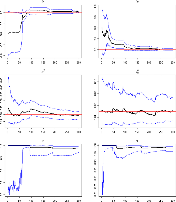
Figure 2: Dynamic factor model (parameter learning). Sequential posterior median (black line) and posterior 95% credibility intervals (blue lines) for model parameters $\beta_{1}$, $\beta_{2}$, $\sigma^{2}$, $\tau^{2}$, $p$ and $q$. True values are the red lines.

Algorithm 2 ((Auxiliary state CDLM)).

Let $z_{t}=(\lambda_{t+1},x_{t},s_{t}^{x},\theta)$.

$\lambda_{t}^{(i)}$ to $\lambda_{t+1}^{(i)}$ via $\lambda_{t+1}^{(i)}\sim p(\lambda_{t+1}|\break(\lambda_{t},\theta)^{(i)})$.

${\tilde{z}}_{t}^{(i)}$ from $z_{t}^{(i)}$ with weights$w_{t+1}^{(i)}\propto p(y_{t+1}|{\tilde{z}}_{t}^{(i)})$.

${\tilde{x}}_{t}^{(i)}$ to $x_{t+1}^{(i)}$ via $p(x_{t+1}|{\tilde{z}}_{t}^{(i)},\break y_{t+1})$.

Sufficient statistics as in PL.

Parameters as in PL.

5 Nonlinear Filtering and Learning

We now extend our PL filter to a general class of nonlinear state space models, namely, the conditional Gaussian dynamic model (CGDM). This class generalizes conditional dynamic linear models by allowing nonlinear evolution equations. In this context we take advantage of most efficiency gains of PL, as we are still able to follow the resample/propagate logic and filter sufficient statistics for $\theta$. Consider a conditional Gaussian state space model with nonlinear evolution equation,

$$\qquad(y_{t+1}|x_{t+1},\lambda_{t+1},\theta) \sim N(F_{\lambda_{t+1}}x_{t+1},V_{\lambda_{t+1}}),$$ (8)

$$(x_{t+1}|x_{t},\lambda_{t+1},\theta) \sim N(G_{\lambda_{t+1}}h(x_{t}),W_{\lambda_{t+1}}),$$ (9)

where $h(\cdot)$ is a given nonlinear function and, again, $\theta$ contains $F$’s, $G$’s, $V$’s and $W$’s. Due to the nonlinearity in the evolution, we are no longer able to work with state sufficient statistics $s_{t}^{x}$, but we are still able to evaluate the predictive $p(y_{t+1}|x_{t},\lambda_{t},\theta)$. In general, take as the particle set the following: $\{(x_{t},\theta,\lambda_{t},s_{t})^{(i)},i=1,\ldots,N\}$. For discrete $\lambda$ we can define the following algorithm:

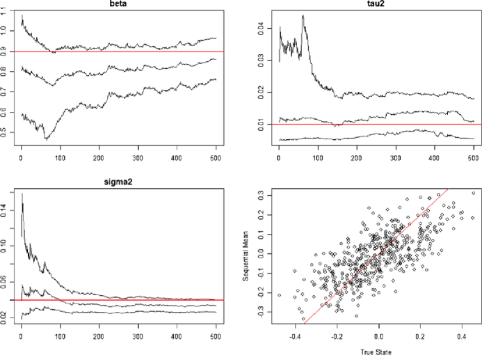
Figure 3: Heavy-tailed non-Gaussian, nonlinear model. Sequential posterior median and posterior 95% credibility intervals (black lines) for model parameters $\beta$, $\sigma^{2}$ and $\tau^{2}$. True values are the red lines. The bottom right panel is the true value of $x_{t}$ against $E(x_{t}|y^{t})$.

Algorithm 3 ((CGDM)).

${\tilde{z}}_{t}^{(i)}$ from $z_{t}^{(i)}=(x_{t},\lambda_{t},\theta)^{(i)}$with weights

$$w_{t}^{(i)}\propto p\bigl{(}y_{t+1}|(x_{t},\lambda_{t},\theta)^{(i)}\bigr{)}.$$

States

$$\lambda_{t+1}^{(i)} \sim p\bigl{(}\lambda_{t+1}|({\tilde{\lambda}}_{t},{\tilde{\theta}})^{(i)},y_{t+1}\bigr{)},$$

$$x_{t+1}^{(i)} \sim p\bigl{(}x_{t+1}|({\tilde{x}}_{t},{\tilde{\theta}})^{(i)},\lambda_{t+1}^{(i)},y_{t+1}\bigr{)}.$$

Parameter sufficient statistics as in Algorithm 1.

Parameters as in PL.

When $\lambda$ is continuous, propagate $\lambda_{t+1}^{(i)}$ from $p(\lambda_{t+1}|\break(\lambda_{t},\theta)^{(i)})$, for $i=1,\ldots,N$, then we resample the particle $(x_{t},\lambda_{t+1},\theta,s_{t})^{(i)}$ with the appropriate predictive distribution $p(y_{t+1}|(x_{t},\lambda_{t+1},\theta)^{(i)})$ as in Algorithm 2. Finally, it is straightforward to extend the backward smoothing strategy of Section 3.3 to obtain samples from $p(x^{T}|y^{T})$.

Example 3 ((Heavy-tailed nonlinear state space model)).

Consider the following non-Gaussian and nonlinear state space model

$$(y_{t+1}|x_{t+1},\lambda_{t+1},\theta) \sim N(x_{t+1},\lambda_{t+1}\sigma^{2}),$$

$$(x_{t+1}|x_{t},\lambda_{t+1},\theta) \sim N(\beta h(x_{t}),\sigma_{x}^{2}),$$

where $\theta=(\beta,\sigma^{2},\tau^{2})$, $h(x_{t})=x_{t}/(1+x_{t}^{2})$ and $\lambda_{t+1}\sim\operatorname{IG}(\nu/2,\nu/2)$, for known $\nu$. Therefore, the distribution of $(y_{t+1}|x_{t+1},\theta)\sim t_{\nu}(x_{t+1},\sigma^{2}),$ that is, a$t$-Student with $\nu$ degrees of freedom.

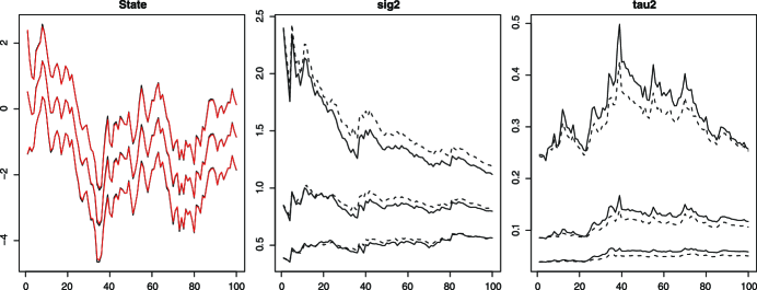
Figure 4: PL and PL with state sufficient statistics (long runs). Left panel—$p(x_{t}|y^{t})$—PL (black), PLsuff (red); Middle panel—$p(\sigma^{2}|y^{t})$—PL (solid line), PLsuff (dotted line); Right panel—$p(\tau^{2}|y^{t})$—PL (solid line), PLsuff (dotted line).

The particle learning algorithm works as follows. Let the particle set $\{(x_{t},\theta,\lambda_{t+1},s_{t})^{(i)}\}_{i=1}^{N}$ approximate $p(x_{t},\theta,\lambda_{t+1},s_{t}|y^{t})$. For anygiven time $t=0,\ldots,\break T-1$ and $i=1,\dots,N$, we first draw an index $k^{i}\sim\operatorname{Mult}(w_{t}^{(1)},\ldots,w_{t}^{(N)})$, with $w_{t}^{(j)}\propto p(y_{t+1}|(x_{t},\lambda_{t+1},\break\theta)^{(j)})$, $j=1,\ldots,N$, and $p(y_{t+1}|x_{t},\lambda_{t+1},\theta)=\break f_{N}(y_{t+1};\beta h(x_{t}),\lambda_{t+1}\sigma^{2}+\tau^{2})$. Then, we draw a new state $x_{t+1}^{(i)}\sim p(x_{t+1}|(\lambda_{t+1},x_{t},\theta)^{(k^{i})},y_{t+1})\equiv f_{N}(x_{t+1};\break\mu_{t+1}^{(i)},V_{t+1}^{(i)})$, where $\mu_{t+1}=V_{t+1}(\lambda_{t+1}^{-1}\sigma^{-2}y_{t+1}+\tau^{-2}\cdot\beta h(x_{t}))$ and $V_{t+1}^{-1}=\lambda_{t+1}^{-1}\sigma^{-2}+\tau^{-2}$. Finally, similar to Example 1, posterior parameter learning for $\theta=(\beta,\sigma^{2},\tau^{2})$ follows directly from a conditionally normal-inverse gamma update. Figure 3 illustrates the above PL algorithm in a simulated example where $\beta=0.9$, $\sigma^{2}=0.04$ and $\sigma^{2}_{x}=0.01$. The algorithm uncovers the true parameters very efficiently in a sequential fashion. In Section 6.1 we revisit this example to compare the performances of PL, MCMC (Carlin, Polson and Stoffer, 1992) and the benchmark particle filter with parameter learning (Liu and West, 2001).

6 Comparing Particle Learning to Existing Methods

We now present a series of examples that illustrate the performance of PL benchmarked by commonly used alternatives.

Example 4 ((State sufficient statistics)).

In this first simulation exercise we revisit the local level model of Example 1 in order to compare PL to its version that takes advantage of state sufficient statistics, that is, by marginalizing the latent states. The main goal is to study the Monte Carlo error of the two filters. We simulated a time series of length $T=100$ with $\sigma^{2}=1$, $\tau^{2}=0.1$ and $x_{0}=0_{p}$. The prior distributions are $\sigma^{2}\sim\operatorname{IG}(5,4)$, $\tau^{2}\sim\operatorname{IG}(5,0.4)$ and $x_{0}\sim N(0,10)$. We run two filters: one with sequential learning for $x_{t}$, $\sigma^{2}$ and $\tau^{2}$ (we call it simply PL), and the other with sequential learning for state sufficient statistics, $\sigma^{2}$ and $\tau^{2}$ (we call it PLsuff). In both cases, the particle filters are based on either one long particle set of size $N=100\mbox{,}000$ (we call it Long) or 20 short particle sets of size $N=5000$ (we call it Short). The results are in Figures 4 to 6. Figure 4 shows that the differences between PL and PLsuff dissipate for fairly large $N$. However, when $N$ is small PLsuff has smaller Monte Carlo error and is less biased than PL, particularly when estimating $\sigma^{2}$ and $\tau^{2}$ (see Figure 5). Similar findings appear in Figure 6 where the mean square errors of the quantiles from the 20 Short runs are compared to those from the Long PLsuff run.

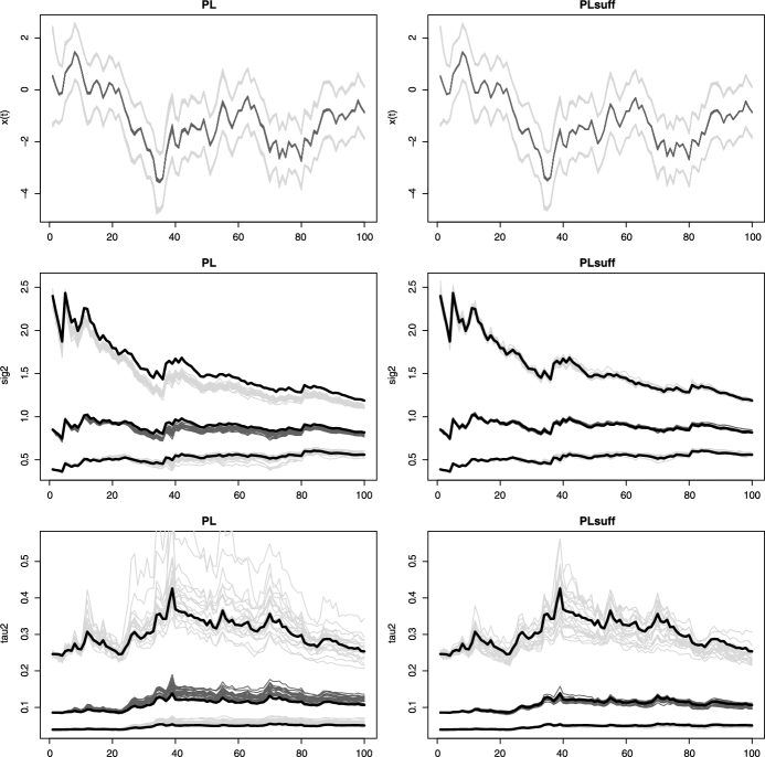
Figure 5: PL and PL with state sufficient statistics (20 short runs). PL runs (left columns) and PLsuff runs (right columns). One long run (black) and 20 short runs (gray); $p(x_{t}|y^{t})$ (top row), $p(\sigma^{2}|y^{t})$ (middle row) and $p(\tau^{2}|y^{t})$ (bottom row).

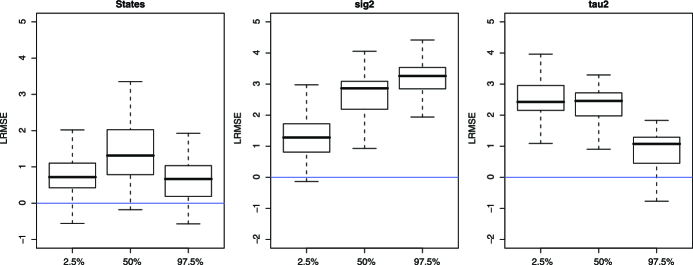
Figure 6: PL and PL with state sufficient statistics (mean square errors). Logarithm of the relative mean square error for three quantiles of $p^{N}(x_{t}|y^{t})$, $p^{N}(\sigma^{2}|y^{t})$ and $p^{N}(\tau^{2}|y^{t})$, averaged across the 20 $N=5000$ runs. PL relative to PLsuff.

Example 5 ((Resample–propagate or propagate–resample?)).

In this second simulation exercise we continue focusing in the local level model of Example 1 to compare PL to three other particle filters: the bootstrap filter (BF), its fully adapted version (FABF), and the auxiliary particle filter (APF) (no fully adapted). BF and FABF are propagate–resample filters, while PL and APF are resample–propagate filters. The main goal is to study the Monte Carlo error of the four filters. We start with the pure case scenario, that is, with fixed parameters. We simulated 20 time series of length $T=100$ from the local level model with parameters $\tau^{2}=0.013$, $\sigma^{2}=0.13$ and $x_{0}=0$. Therefore, the signal to noise ratio $\sigma_{x}/\sigma$ equals $0.32$. Other combinations were also tried and similar results were found. The prior distribution of the initial state $x_{0}$ was set at $N(0,10)$. For each time series, we run 20 times on each of the four filters, all based on $N=1000$ particles. We use five quantiles to compare the various filters. Let $q_{\alpha}^{t}$ be such that $\operatorname{Pr}(x_{t}<q^{\alpha}_{t}|y^{t})=\alpha$, for $\alpha=(0.05,0.25,0.5,0.75,0.95)$. Then, the mean square error (MSE) for filter $f$, at time $t$ and quantile $\alpha$ is

$$\mathit{MSE}^{\alpha}_{t,f}=\frac{1}{400}\sum_{d=1}^{20}\sum_{r=1}^{20}(q^{\alpha}_{t,d}-{\hat{q}}^{\alpha}_{t,d,f,r})^{2},$$

where $d$ and $r$ index the data set and the particle filter run, respectively. We compare PL, APF and FABF via logarithm relative MSE (LRMSE), relative to the benchmark BF. Results are summarized in Figure 7. PL is uniformly better than all three alternatives. Notice that the only algorithmic difference between PL and FABF is that PL reverses the propagate–resample steps.

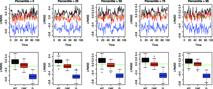
Figure 7: APF, FABF and PL pure filter. Logarithm of the relative mean square error for five quantiles of $p^{N}(x_{t}|y^{t})$. MSE relative to BF. Boxplots on the second row are based on the time series plots on the first row.

We now move to the parameter learning scenario, where $\sigma^{2}$ is still kept fixed but learning of $\tau^{2}$ is performed. Three time series of length $T=1000$ were simulated from the local level model with $x_{0}=0$ and $(\sigma^{2},\tau^{2})$ in $\{(0.1,0.01),(0.01,0.01),(0.01,0.1)\}$. The independent prior distributions for $x_{0}$ and $\tau^{2}$ are $x_{0}\sim N(0,1)$ and $\tau^{2}\sim\operatorname{IG}(10,9\tau_{0}^{2})$, where $\tau_{0}^{2}$ is the true value of $\tau^{2}$ for a given time series. In all filters $\tau^{2}$ is sampled offline from $p(\tau^{2}|s_{t})$ where $s_{t}$ is the vector of conditional sufficient statistics. We run the filters 100 times, all with the same seed within run, for each one of the three simulated data sets. Finally, the number of particles was set at $N=5000$, with similar results found for smaller $N$, ranging from 250 to 2000 particles. Mean absolute errors (MAE) over the 100 replications are constructed by comparing quantiles of the true sequential distributions $p(x_{t}|y^{t})$ and $p(\tau^{2}|y^{t})$ to quantiles of the estimated sequential distributions $p^{N}(x_{t}|y^{t})$ and $p^{N}(\tau^{2}|y^{t})$. More specifically, for time $t$, $a$ in $\{x,\tau^{2}\}$, $\alpha$ in $\{0.01,0.50,0.99\}$, true quantiles $q_{t,a}^{\alpha}$ and PL quantiles ${\hat{q}}_{t,a,r}^{\alpha}$,

$$\mathit{MAE}_{t,a}^{\alpha}=\frac{1}{100}\sum_{r=1}^{100}|q_{t,a}^{\alpha}-{\hat{q}}_{t,a,r}^{\alpha}|.$$

Across different quantiles and combinations of error variances, PL is at least as good as FABF and in many cases significantly better than BF. Results appear in Figure 8.

Figure 8: BF, FABF and PL with learning of $\tau^{2}$. Mean absolute errors. BF (black), FABF (red) and PL (blue).

Example 6 ((PL versus LW)).

Consider once again a variation of the dynamic linear model introduced in Example 1, but now we assume complete knowledge about $(\sigma^{2},\tau^{2})$ in

$$(y_{t+1}|x_{t+1},\beta) \sim N(x_{t},\sigma^{2}),$$

$$(x_{t+1}|x_{t},\beta) \sim N(\beta x_{t},\tau^{2})$$

for $t=1,\ldots,T=100$, $\sigma^{2}=1$, $x_{1}=0.0$ and three possible values for $\tau^{2}=(0.01,0.25,1.00)$. So, the signal to noise ratio $\tau/\sigma=0.1,0.5,1.0$. Only $\beta$ and $x_{t}$ are sequentially estimated and their independent prior distributions are $N(1.0,1.0)$ and $N(0.0,1.0)$, respectively. The particle set has length $N=2000$ and both filters were run $50$ times to study the size of the Monte Carlo error. The smoothing parameter $\delta$ of Liu and West’s filter was set at $\delta=0.95$, but fairly similar results were found for $\delta$ ranging from $0.8$ to $0.99$. Our findings, summarized in Figure 9, favor PL over LW uniformly across all scenarios. The discrepancy is higher when $\tau/\sigma$ is small, which is usually the case in state space applications.

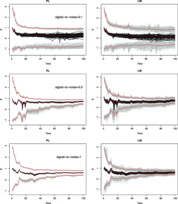
Figure 9: PL and LW (parameter learning). Posterior mean and 95% credibility interval from $p(\beta|y^{t})$. Medians across the 50 runs appear in red. $N=2000$ particles. signal-to-noise stands for $\sigma_{x}/\sigma$. In all cases, $\sigma=1$.

Figure 10: PL and FFBS (smoothed distributions). $T=100$ simulated from a local level model with $\sigma^{2}=1$, $\tau^{2}=0.5$, $x_{0}=0$ and $x_{0}\sim N(0,100)$. PL is based on $N=1000$ particles, while FFBS is based on $2N$ draws with the first $N$ discarded.

6.1 PL vs MCMC

PL combined with the backward smoothing algorithm (as in Section 3.3) is an alternative to MCMC methods for state space models. In general, MCMC methods (see Gamerman and Lopes, 2006) useMarkov chains designed to explore the posterior distribution $p(x^{T},\theta|y^{T})$ of states and parameters conditional on all the information available, $y^{T}=(y_{1},\ldots,\break y_{T})$. For example, an MCMC strategy would have to iterate through

$$p(\theta|x^{T},y^{T})\quad\mbox{and}\quad p(x^{T}|\theta,y^{T}).$$

However, MCMC relies on the convergence of very high-dimensional Markov chains. In the purely conditional Gaussian linear models or when states are dicrete, $p(x^{T}|\theta,y^{T})$ can be sampled in block using FFBS. Even in these ideal cases, achieving convergency is far from an easy task and the computational complexity is enormous, as at each iteration one would have to filter forward and backward sample for the full state vector $x^{T}$. The particle learning algorithm presented here has two advantages: (i) it requires only one forward/backward pass through the data for all $N$ particles and (ii) the approximation accuracy does not rely on convergence results that are virtually impossible to assess in practice (see Papaspiliopoulos and Roberts, 2008).

In the presence of nonlinearities, MCMC methods will suffer even further, as no FFBS scheme is available for the full state vector $x^{T}$. One would have to resort to univariate updates of $p(x_{t}|x_{(-t)},\theta,y^{T})$ as in Carlin, Polson and Stoffer (1992), where $x_{(-t)}$ is $x^{T}$ without $x_{t}$. It is well known that these methods generate very “sticky” Markov chains, increasing computational complexity and slowing down convergence. PL is also attractive given the simple nature of its implementation (especially if compared to more novel hybrid methods).

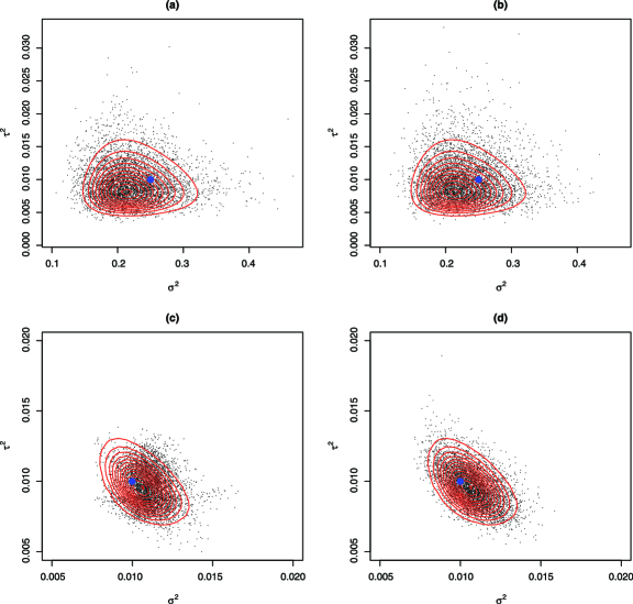
Figure 11: PL and FFBS (parameter learning). Contour plots for the true posterior $p(\sigma^{2},\tau^{2}|y^{T})$ (red contours) and posterior draws from PL, panels (a) and (c), and FFBS, panels (b) and (d). The blue dots represent the true value of the pair $(\sigma^{2},\tau^{2})$. The sample size is $T=50$ (top row) and $T=500$ (bottom row).

Example 7 ((PL versus FFBS)).

We revisit the first order dynamic linear model introduced in Example 1 to compare our PL smoother and the forward-filtering, backward-sampling (FFBS) smoother. Assuming knowledge about $\theta$, Figure 10 compares the true smoothed distributions $p(x_{t}|y^{T})$ to approximations based on PL and on FFBS. Now, when parameter learning is introduced, PL performance is comparable to that of the FFBS when approximating $p(\sigma^{2},\tau^{2}|y^{T})$, as shown in Figure 11. We argue that, based on these empirical findings, PL and FFBS are equivalent alternatives for posterior computation. We now turn to the issue of computational cost, measured here by the running time in seconds of both schemes. Data was simulated based on $(\sigma^{2},\tau^{2},x_{0})=(1.0,0.5,0.0)$. The prior distribution of $x_{0}$ is $N(0,100)$, while $\sigma^{2}$ and $\tau^{2}$ are kept fixed throughout this exercise. PL was based on $N$ particles and FFBS based on $2N$ iterations, with the first $M$ discarded. Table 1 summarizes the results. For fixed $N$, the (computational) costs of both PL and FFBS increase linearly with $T$, with FFBS twice as fast as PL. For fixed $T$, the cost of FFBS increases linearly with $N$, while the cost of PL increases exponentially with $N$. These findings were anticipated in Section 3.3. As expected, PL outperforms FFBS when comparing filtering times.

Example 8 ((PL versus single-move MCMC)).

Our final example compares PL to a single-move MCMC as in Carlin, Polson and Stoffer (1992). We consider the first order conditional Gaussian dynamic model with nonlinear state equation as defined in Example 3. The example focuses on the estimation of $\sigma^{2}$. We generate data with different levels of signal to noise ratio and compare the performance of PL versus MCMC. Table 2 presents the results for the comparisons. Once again, PL provides significant improvements in computational time and MC variability for parameter estimation over MCMC.

Table 1: Computing time (in seconds) of PL and FFBS for smoothing. In parenthesis are PL times for filtering

$\bolds{N=500}$			$\bolds{T=100}$
1-3,4-6 $\bolds{T}$	PL	FFBS	$\bolds{N}$	PL	FFBS
200	18.8 (0.25)	09.1	0500	009.3 (0.09)	04.7
500	47.7 (1.81)	23.4	1000	032.8 (0.15)	09.6
1000	93.9 (8.29)	46.1	2000	127.7 (0.34)	21.7

Table 2: Single-move MCMC based on 2000 draws, after 2000 burn-in. PL based on 2000 particles. Expectations are with respect to the whole data set at time $T$, while the true value of $\tau^{2}$ is $0.01$. Numbers in parenthesis are 1000 times the standard deviation based on 20 replications of the algorithms. Time is in seconds when running our code in R version 2.8.1 on a MacBook with a 2.4 GHz processor and 4 GB MHz of memory

$\bolds{T}$	$\bolds{\sigma^{2}}$	Time	$\bolds{E(\sigma^{2})}$	$\bolds{E(\tau^{2})}$
Single-move MCMC
50	0.2500	19.7	0.209934 (3.901)	0.011 (1.532)
	0.0100	19.3	0.009151 (0.253)	0.008 (0.545)
	0.0001	19.3	0.000097 (0.003)	0.010 (0.049)
200	0.2500	79.3	0.249059 (6.981)	0.027 (12.76)
	0.0100	79.1	0.009740 (0.305)	0.013 (1.375)
	0.0001	79.8	0.000099 (0.004)	0.011 (0.032)
PL
50	0.2500	00.8	0.170576 (1.633)	0.010 (0.419)
	0.0100	00.7	0.007204 (0.151)	0.008 (0.165)
	0.0001	00.6	0.000092 (0.004)	0.010 (0.058)
200	0.2500	06.5	0.262396 (6.392)	0.009 (1.332)
	0.0100	06.4	0.010615 (0.570)	0.011 (0.935)
	0.0001	06.4	0.000098 (0.010)	0.011 (0.057)

7 Final Remarks

In this paper we provide particle learning tools (PL) for a large class of state space models. Our methodology incorporates sequential parameter learning, state filtering and smoothing. This provides an alternative to the popular FFBS/MCMC (Carter and Kohn, 1994) approach for conditional dynamic linear models (DLMs) and also to MCMC approaches to nonlinear non-Gaussian models. It is also a generalization of the mixture Kalman filter (MKF) approach of Chen and Liu (2000) that includes parameter learning and smoothing. The key assumption is the existence of a conditional sufficient statistic structure for the parameters which is commonly available in many commonly used models.

We provide extensive simulation evidence to address the efficiency of PL versus standard methods. Computational time and accuracy are used to assess the performance. Our approach compares very favorably with these existing strategies and is robust to particle degeneracies as the sample size grows. Finally, PL has the additional advantage of being an intuitive and easy-to-implement computational scheme and should, therefore, become a default choice for posterior inference in a variety of models, with examples already appearing in Lopes et al. (2010), Carvalho et al. (2009), Prado and Lopes (2010), Lopes and Tsay (2010) and Lopes and Polson (2010).

References

- (1) Briers, M., Doucet, A. and Maskell, S. (2010). Smoothing algorithms for state-space models. Ann. Inst. Statist. Math. 62 61–89. \MR2577439
- (2) Cappé, O., Godsill, S. and Moulines, E. (2007). An overview of existing methods and recent advances in sequential Monte Carlo. IEEE Proceedings 95 899–924.
- (3) Carlin, B., Polson, N. G. and Stoffer, D. (1992). A Monte Carlo approach to nonnormal and nonlinear state-space modeling. J. Amer. Statist. Assoc. 87 493–500.
- (4) Carter, C. and Kohn, R. (1994). On Gibbs sampling for state space models. Biometrika 82 339–350. \MR1311096
- (5) Carvalho, C. M. and Lopes, H. F. (2007). Simulation-based sequential analysis of Markov switching stochastic volatility models. Comput. Statist. Data Anal. 51 4526–4542. \MR2364463
- (6) Carvalho, C. M., Lopes, H. F., Polson, N. G. and Taddy, M. (2009). Particle learning for general mixtures. Working paper, Univ. Chicago Booth School of Business.
- (7) Chen, R. and Liu, J. (2000). Mixture Kalman filters. J. Roy. Statist. Soc. Ser. B 62 493–508. \MR1772411
- (8) Doucet, A., de Freitas, J. and Gordon, N. (2001). Sequential Monte Carlo Methods in Practice. Springer, New York. \MR1847783
- (9) Fearnhead, P. (2002). Markov chain Monte Carlo, sufficient statistics, and particle filters. J. Comput. Graph. Statist. 11 848–862. \MR1951601
- (10) Fearnhead, P., Wyncoll, D. and Tawn, J. (2008). A sequential smoothing algorithm with linear computational cost. Working paper, Dept. Mathematics and Statistics, Lancaster Univ.
- (11) Frühwirth-Schnatter, S. (1994). Applied state space modelling of non-Gaussian time series using integration-based Kalman filtering. Statist. Comput. 4 259–269.
- (12) Gamerman, D. and Lopes, H. F. (2006). Markov Chain Monte Carlo: Stochastic Simulation for Bayesian Inference. Chapman & Hall/CRC Press, Boca Raton, FL. \MR2260716
- (13) Godsill, S. J., Doucet, A. and West, M. (2004). Monte Carlo smoothing for nonlinear time series. J. Amer. Statist. Assoc. 99 156–168. \MR2054295
- (14) Gordon, N., Salmond, D. and Smith, A. F. M. (1993). Novel approach to nonlinear/non-Gaussian Bayesian state estimation. IEE Proceedings-F 140 107–113.
- (15) Johannes, M. and Polson, N. G. (2008). Exact particle filtering and learning. Working paper, Univ. Chicago Booth School of Business.
- (16) Johannes, M., Polson, N. G. and Yae, S. M. (2008). Nonlinear filtering and learning. Working paper, Univ. Chicago Booth School of Business.
- (17) Kalman, R. E. (1960). A new approach to linear filtering and prediction problems. Transactions of the ASME—Journal of Basic Engineering 82 35–45.
- (18) Liu, J. and Chen, R. (1998). Sequential Monte Carlo methods for dynamic systems. J. Amer. Statist. Assoc. 93 1032–1044. \MR1649198
- (19) Liu, J. and West, M. (2001). Combined parameters and state estimation in simulation-based filtering. In Sequential Monte Carlo Methods in Practice (A. Doucet, N. de Freitas and N. Gordon, eds.). Springer, New York. \MR1847793
- (20) Lopes, H. F. and Polson, N. G. (2010). Extracting SP500 and NASDAQ volatility: The credit crisis of 2007–2008. In Handbook of Applied Bayesian Analysis (A. O’Hagan and M. West, eds.) 319–342. Oxford Univ. Press, Oxford.
- (21) Lopes, H. F. and Tsay, R. E. (2010). Bayesian analysis of financial time series via particle filters. J. Forecast. To appear.
- (22) Lopes, H. F., Carvalho, C. M., Johannes, M. and Polson, N. G. (2010). Particle learning for sequential Bayesian computation. In Bayesian Statistics 9 (J. M. Bernardo, M. J. Bayarri, J. O. Berger, A. P. Dawid, D. Heckerman, A. F. M. Smith and M. West, eds.). Oxford Univ. Press, Oxford.
- (23) Papaspiliopoulos, O. and Roberts, G. (2008). Stability of the Gibbs sampler for Bayesian hierarchical models. Ann. Statist. 36 95–117. \MR2387965
- (24) Pitt, M. and Shephard, N. (1999). Filtering via simulation: Auxiliary particle filters. J. Amer. Statist. Assoc. 94 590–599. \MR1702328
- (25) Polson, N. G., Stroud, J. and Müller, P. (2008). Practical filtering with sequential parameter learning. J. Roy. Statist. Soc. Ser. B 70 413–428. \MR2424760
- (26) Prado, R. and Lopes, H. F. (2010). Sequential parameter learning and filtering in structured autoregressive models. Working paper, Univ. Chicago Booth School of Business.
- (27) Storvik, G. (2002). Particle filters in state space models with the presence of unknown static parameters. IEEE Trans. Signal Process. 50 281–289.
- (28) West, M. (1986). Bayesian model monitoring. J. Roy. Statist. Soc. Ser. B 48 70–78. \MR0848052
- (29) West, M. and Harrison, J. (1997). Bayesian Forecasting and Dynamic Models, 2nd ed. Springer, New York. \MR1482232