Featureless 2D-3D Pose Estimation by
Minimising an Illumination-Invariant Loss
 

Abstract

The problem of identifying the 3D pose of a known object from a given 2D image has important applications in Computer Vision ranging from robotic vision to image analysis. Our proposed method of registering a 3D model of a known object on a given 2D photo of the object has numerous advantages over existing methods: It does neither require prior training nor learning, nor knowledge of the camera parameters, nor explicit point correspondences or matching features between image and model. Unlike techniques that estimate a partial 3D pose (as in an overhead view of traffic or machine parts on a conveyor belt), our method estimates the complete 3D pose of the object, and works on a single static image from a given view, and under varying and unknown lighting conditions. For this purpose we derive a novel illumination-invariant distance measure between 2D photo and projected 3D model, which is then minimised to find the best pose parameters. Results for vehicle pose detection are presented.

Contents

1. 1 Introduction
2. 2 Related Work
3. 3 Matching 3D Models with 2D Photos
4. 4 Derivation of Invariant Loss Function
5. 5 Practical Behaviour of the Loss Function
6. 6 Optimising Vehicle Pose using the Loss Function
7. 7 Technical Aspects
8. 8 Discussion

Keywords

illumination-invariant loss; 2D-3D pose estimation; pixel-based; featureless; optimisation.

1 Introduction

Pose estimation is a fundamental component of many computer vision applications, ranging from robotic vision to intelligent image analysis. In general, pose estimation refers to the process of obtaining the location and orientation of an object. However, the accuracy and nature of the pose estimate required varies from application to application. Certain applications require the estimation of the full 3D pose of an object, while other applications require only a subset of the pose parameters.

Motivation. The 2D-3D registration problem in particular is concerned with estimating the pose parameters that describe a 3D object model within a given 2D scene. An image/photograph of a known object can be analysed in greater detail if a 3D model of the object can be registered over it, to be used as a ground truth. As an example, consider the case of automatically analysing a damaged car using a photograph. The focus of this work is to develop a method to estimate the pose of a known 3D object model in a given 2D image, with an emphasis on estimating the pose of cars. We have the following objectives in mind.

• Use only a single, static image limited to a single view

• Work with any unknown camera (without prior camera calibration)

• Avoid user interaction

• Avoid prior training / learning

• Work under varying and unknown lighting conditions

• Estimate the full 3D pose of the object (not a partial pose as in an overhead view of traffic or machine parts along a conveyor belt)

A 3D pose estimation method with these properties would also be useful in remote sensing, automated scene recognition and computer graphics, as it allows for additional information to be extracted without the need for human involvement.

Many methods, including point correspondence based methods, implicit shape model based methods and image gradient based methods, have been developed to solve the pose estimation problem. However, the methods identified in the literature do not satisfy the objectives mentioned above, hence the necessity of our novel method. A more detailed review of existing pose estimation methods ranging over the past 30 years is presented in Section 2.

Main contribution. This paper presents a method which registers a known 3D model onto a given 2D photo containing the modelled object while satisfying the objectives outlined above. It does this by measuring the closeness of the projected 3D model to the 2D photo on a pixel (rather than feature) basis. Background and unknown lighting conditions of the photo are major complications, which prevent using a naive image difference like the absolute or square loss as a measure of fit.

A major contribution of this paper is the novel “distance” measure in Section 3 that does neither depend on the lighting of the real scene in the photo nor on choosing an appropriate lighting in the rendering of the 3D model, hence does not require knowledge of the lighting. Technically, we derive in Section 4 a loss function for vector-valued pixel attributes (of different modality) that is invariant under linear transformations of the attributes.

To analyse the nature of the developed loss function, we have applied it to a series of test cases of varying complexity, as detailed in Section 5. These test cases indicate that for our target application the loss function is well behaved and can be optimised using a standard optimisation method to find an accurate pose match. As presented in Section 6, we achieve good pose recovery results in both artificial and real world test cases using this optimisation scheme. In these optimisation tests, negative influence of the background is attenuated by clipping the photo to the projection of the 3D model when calculating the loss. Technical aspects of the optimisation and loss calculation methods are discussed in Section 7.

2 Related Work

Model based object recognition has received considerable attention in computer vision circles. A survey by Chin and Dyer [CD86] shows that model based object recognition algorithms generally fall into 3 categories, based on the type of object representation used - namely 2D representations, 2.5D representations or 3D representations.

2D representations store the information of a particular 2D view of an object (a characteristic view) as a model and use this information to identify the object from a 2D image. Global feature methods have been used by Gleason and Algin [GA79] to identify objects like spanners and nuts on a conveyor belt. Such methods use features such as the area, perimeter, number of holes visible and other global features to model the object. Structural features like boundary segments have been used by Perkins [Per78] to detect machine parts using 2D models. A relational graph method has been used by Yachida and Tsuji [YT77] to match objects to a 2D model using graph matching techniques. These 2D representation-based algorithms require prior training of the system using a ‘show by example’ method.

2.5D approaches are also viewer centred, where the object is known to occur in a particular view. They differ from the 2D approach as the model stores additional information such as intrinsic image parameters and surface-orientation maps. The work done by Poje and Delp [Poj82] explain the use of intrinsic scene parameters in the form of range (depth) maps and needle (local surface orientation) maps. Shape from shading [Hor75] and photometric stereo [Woo78] are some other examples of the use of the 2.5D approach used for the recognition of industrial parts. A range of techniques for such 2D/2.5D representations are described by Forsythe and Ponce [FP02], by posing the object recognition problem as a correspondence problem. These methods obtain a hypothesis based on the correspondences of a few matching points in the image and the model. The hypothesis is validated against the remaining known points.

3D approaches are utilised in situations where the object of interest can appear in a scene from multiple viewing angles. Common 3D representation approaches can be either an ‘exact representation’ or a ‘multi-view feature representation’. The latter method uses a composite model consisting of 2D/2.5D models for a limited set of views. Multi-view feature representation is used along with the concept of generalised cylinders by Brooks and Binford [Bro81] to detect different types of industrial motors in the so called ACRONYM system. The models used in the exact representation method, on the contrary, contain an exact representation of the complete 3D object. Hence a 2D projection of the object can be created for any desired view. Unfortunately, this method is often considered too costly in terms of processing time.

Limitations. The 2D and 2.5D representations are insufficient for general purpose applications. For example, a vehicle may be photographed from an arbitrary view in order to indicate the damaged parts. Similarly, the 3D multi-view feature representation is also not suitable, as we are not able to limit the pose of the vehicle to a small finite set of views. Therefore, pose identification has to be done using an exact 3D model. Little work has been done to date on identifying the pose of an exact 3D model from a single 2D image. Huttenlocher and Ullman [HU90] use a 3D model that contains the locations of edges. The edges/contours identified in the 2D image are matched against the edges in the 3D model to calculate the pose of the object. The method has been implemented for simple 3D objects. However, this method will not work well on objects with rounded surfaces without clearly identifiable edges.

Implicit Shape Models. Recent work by Arie-Nachimson and Ronen Basri [ANB09] makes use of ‘implicit shape models’ to recognise 3D objects from 2D images. The model consists of a set of learned features, their 3D locations and the views in which they are visible. The learning process is further refined using factorisation methods. The pose estimation consists of evaluating the transformations of the features that give the best match. A typical model requires around 65 images to be trained. There are many different types of cars in use and new car models are manufactured quite frequently. Therefore, any methodology that requires training car models would be laborious and time consuming. Hence, a system that does not require such training is preferred for the problem at hand.

Image gradients. Gray scale image gradients have been used to estimate the 3D pose in traffic video footage from a stationary camera by Kollnig and Nagel [KN97]. The method compares image gradients instead of simple edge segments, for better performance. Image gradients from projected polyhedral models are compared against image gradients in video images. The pose is formulated using 3 degrees of freedom; 2 for position and 1 for angular orientation. Tan and Baker [TB00] use image gradients and a Hough transform based algorithm for estimating vehicle pose in traffic scenes, once more describing the pose via 3 degrees of freedom. Pose estimation using 3 degrees of freedom is adequate for traffic image sequences, where the camera position remains fixed with respect to the ground plane. This approach does not provide a full pose estimate required for a general purpose application.

Feature-based methods. Work done by [DDDS04] and later by [MNLF] attempt to simultaneously solve the pose and point correspondence problems. The success of these methods are affected by the quality of the features extracted from the object, which is non-trivial with objects like cars. Our method on the contrary, does not depend on feature extraction.

Distance metrics can be used to represent a distance between two data sets, and hence give a measure of their similarity. Therefore, distance metrics can be used to measure similarity between different 2D images, as well as 2D images and projections of a 3D model. A basic distance metric would be the Euclidian Distance or the 2-norm $||\cdot||_{2}$. However, this has the disadvantage of being dependant on the scale of measurement. The Mahalanobis Distance on the other hand, is a scale-invariant distance measure. It is defined as

$$||x-y||_{C^{-1}}\equiv\sqrt{(x-y)^{\mskip-3.0mu\top\mskip-3.0mu}C^{-1}(x-y)}$$

for random vectors $x$ and $y$ with a covariance matrix of $C$. The Mahalanobis distance will reduce to the Euclidean distance when the covariance matrix is the identity matrix ($C=I$). The Mahalanobis distance is used by Xing et al. [XNJR03] for clustering. It is also used by Deriche and Faugeras [DF90] to match line segments in a sequence of time varying images.

3 Matching 3D Models with 2D Photos

We describe our approach of matching 3D models to 2D photos in this section using a novel illumination-invariant loss function. A detailed derivation of the loss is provided in Section 4.

The problem. Assume we want to match a 3D model ($M$) to a 2D photo ($F$) or vice versa. More precisely, we have a 3D model (e.g. as a triangulated textured surface) and we want to find a projection $\theta$ for which the rendered 2D image $M_{\theta}$ has the same perspective as the 2D photo $F$. As long as we do not know the lighting conditions of $F$, we cannot expect $F$ to be close to $M_{\theta}$, even for the correct $\theta$. Indeed, if the light in $F$ came from the right, but the light shines on $M$ from the left, $M_{\theta}$ may be close to the negative of $F$.

Setup. Formally, let $P=Z\mskip-3.0mu\mskip-3.0mu\mskip-3.0muZ_{n_{x}}\times Z\mskip-3.0mu\mskip-3.0mu\mskip-3.0muZ_{n_{y}}=\{1,...,n_{x}\}\times\{1,...,n_{y}\}$ be the set of $|P|$ (integer) pixel coordinates, and $p=(x,y)\in P$ be a pixel coordinate. Alternatively a smaller region of interest may be used for $P$ instead of $Z\mskip-3.0mu\mskip-3.0mu\mskip-3.0muZ_{n_{x}}\times Z\mskip-3.0mu\mskip-3.0mu\mskip-3.0muZ_{n_{y}}$ as explained in Section 6. Let $F:P\to I\mskip-3.0mu\mskip-3.0muR^{n}$ be a photo with $n$ real pixel attributes, and $M_{\theta}:P\to I\mskip-3.0mu\mskip-3.0muR^{m}$ a projection of a 3D object to a 2D image with $m$ real pixel attributes. The attributes may be colours, local texture features, surface normals, or else. In the following we consider the case of grey-level photos ($n=1$), and for reasons that will become clear, use surface normals and brightness $(m=4)$ of the (projected) 3D model.

Lambertian reflection model. A simple Lambertian reflection model is not realistic enough to result in a zero loss on real photos, even at the correct pose. Nevertheless (we believe and experimentally confirm that) it results in a minimum at the correct pose, which is sufficient for matching purposes. We use Phong shading without specular reflection for this purpose [FvDFH95]. Let $I_{a/d}\in I\mskip-3.0mu\mskip-3.0muR$ be the global ambient/diffuse light intensities of the 3D scene, and $\boldsymbol{L}\in I\mskip-3.0mu\mskip-3.0muR^{3}$ be the (global) unit vector in the direction of the light source (or their weighted sum in case of multiple sources). For reasons to become clear later, we introduce an extra illumination offset $I_{0}\in I\mskip-3.0mu\mskip-3.0muR$ (which is 0 in the Phong model). For each surface point $p$, let $k_{a/d}(p)\in I\mskip-3.0mu\mskip-3.0muR$ be the ambient/diffuse reflection constants (intrinsic surface brightness) and $\boldsymbol{\phi}(p)\in I\mskip-3.0mu\mskip-3.0muR^{3}$ be the unit (interpolated) surface “normal” vector. Then the apparent intensity $I$ of the corresponding point $p$ in the projection $M_{\theta}(p)$ is [FvDFH95]

$$I(p)=k_{a}(p)I_{a}\mskip-3.0mu+\mskip-3.0muk_{d}(p)(\boldsymbol{L}^{\mskip-3.0mu\top\mskip-3.0mu}\boldsymbol{\phi}(p))I_{d}\mskip-3.0mu+\mskip-3.0muI_{0}\equiv A\mskip-3.0mu\cdot\mskip-3.0muM_{\theta}(p)\mskip-3.0mu+\mskip-3.0mub$$

The last expression is the same as the first, just written in a more covariant form: $M_{\theta}(p):=(k_{a}(p),k_{d}(p)\boldsymbol{\phi}(p))^{\mskip-3.0mu\top\mskip-3.0mu}\in I\mskip-3.0mu\mskip-3.0muR^{4}$ are the known surface (dependent) parameters, and $A:=(I_{a},I_{d}\boldsymbol{L}^{\mskip-3.0mu\top\mskip-3.0mu})\in I\mskip-3.0mu\mskip-3.0muR^{4\times 1}$ are the four (unknown) global illumination constants, and $b=I_{0}$. Since $I(\cdot)$ is linear in $A$ and $M_{\theta}(\cdot)$, any rendering is a simple global linear function of $M_{\theta}(p)$. This model remains exact even for multiple light sources and can easily be generalised to color models and color photos.

Illumination invariant loss. We measure the closeness of the projected 3D model $M_{\theta}$ to the 2D photo $F$ by some distance $D(F,AM_{\theta}+b)$, e.g. square or absolute or Mahalanobis. We do not want to assume any extra knowledge like the lighting conditions $A$ under which the photo has been taken, which rules out a direct use of $D$. Ideally we want a “distance” between $F$ and $M$ that is independent of $A$ and is zero if and only if there exists a lighting condition $A$ such that $F$ and $AM_{\theta}+b$ coincide.

Indeed, this is possible, if (rather than defining $M_{\theta}$ as some $A$-dependent rendered projection of $M$) we use $A$-independent brightness and normals $M_{\theta}$ as pixel features as defined above, and define a linearly invariant distance as follows: Let

$$\bar{F}\mskip 5.0mu plus 5.0mu:=\mskip 5.0mu plus 5.0mu{1\over|P|}\sum_{p\in P}F(p)\mskip 5.0mu plus 5.0mu\in I\mskip-3.0mu\mskip-3.0muR{\quad\mbox{and}\quad}\bar{M}_{\theta}\mskip 5.0mu plus 5.0mu:=\mskip 5.0mu plus 5.0mu{1\over|P|}\sum_{p\in P}M_{\theta}(p)\mskip 5.0mu plus 5.0mu\in I\mskip-3.0mu\mskip-3.0muR^{4}$$

be the average attribute values of photo and projection, and

$$C_{FM_{\theta}}:={1\over|P|}\sum_{p\in P}(F(p)-\bar{F})(M_{\theta}(p)-\bar{M}_{\theta})^{\mskip-3.0mu\top\mskip-3.0mu}\mskip 5.0mu plus 5.0mu\in I\mskip-3.0mu\mskip-3.0muR^{1\times 4}$$

be the cross-covariance matrix between $F$ and $M_{\theta}$ and similarly $C_{M_{\theta}F}=C_{FM_{\theta}}^{\mskip-3.0mu\top\mskip-3.0mu}\in I\mskip-3.0mu\mskip-3.0muR^{4\times 1}$ and the covariance matrices $C_{FF}\in I\mskip-3.0mu\mskip-3.0muR^{1\times 1}$ and $C_{M_{\theta}M_{\theta}}\in I\mskip-3.0mu\mskip-3.0muR^{4\times 4}$. With this notation we can define the following distance or loss function between $F$ and $M_{\theta}$:

$$\mbox{Loss}(\theta):=\min\{n,m\}-\mbox{tr}[C_{FM_{\theta}}C_{M_{\theta}M_{\theta}}^{-1}C_{M_{\theta}F}C_{FF}^{-1}]$$ (1)

Obviously this expression is independent of $A$. In the next section we show that it is invariant under regular linear transformation of the pixel/attribute values of $F$ and $M_{\theta}$ and zero if and only if there is a perfect linear transformation of the pixel values from $M_{\theta}$ to $F$. This makes it unnecessary to know the exact surface reflection constants of the object ($k_{a/d}(p)\in I\mskip-3.0mu\mskip-3.0muR$). We will actually derive

$$\mbox{Loss}(\theta)=\smash{\min_{A,b}}\mskip 3.0muD_{\text{Mahalanobis}}(F,A\mskip-3.0mu\cdot\mskip-3.0muM_{\theta}+b)$$

This implies that $\mbox{Loss}(\theta)$ is zero if and only if there is a lighting $A$ under which $F$ and $M_{\theta}$ coincide, which we desired.

4 Derivation of Invariant Loss Function

A detailed derivation of the loss function is given in this section. Although together with Section 3, this is a main novel contribution of this paper, it may be skipped over by the more application-oriented reader without affecting the continuity of the rest of the paper.

Notation. Using the notation of the previous section, we measure the similarity of photo $F:P\to I\mskip-3.0mu\mskip-3.0muR^{n}$ and projected 3D model $M_{\theta}:P\to I\mskip-3.0mu\mskip-3.0muR^{m}$ (returning to general $n,m\in I\mskip-3.0mu\mskip-3.0muN$) by some loss:

$$\mbox{Loss}(\theta):=D(F,M_{\theta}):={1\over|P|}\smash{\sum_{p\in P}}d(F(p),M_{\theta}(p))$$ (2)

where $d$ is a distance measure between corresponding pixels of the two images to be determined below. A very simple, but as discussed in Section 2 for our purpose unsuitable, choice in case of $m=n$ would be the square loss $d(F(p),M_{\theta}(p))=||F(p)-M_{\theta}(p)||_{2}^{2}$.

It is convenient to introduce the following probability notation: Let $\omega$ be uniformly distributed in $P$, i.e. $\text{Pr}[\omega]=|P|^{-1}$. Define the vector random variables $X:=F(\omega)\in I\mskip-3.0mu\mskip-3.0muR^{n}$ and $Y:=M_{\theta}(\omega)\in I\mskip-3.0mu\mskip-3.0muR^{m}$. The expectation of a function of $X$ and $Y$ then is

$${\bf E}[g(X,Y)]:={1\over|P|}\sum_{\omega\in P}g(X(\omega),Y(\omega))$$

With this notation, (2) can be written as

$$\mbox{Loss}(\theta)=D(X,Y)={\bf E}[d(X,Y)]$$

Noisy (un)known relation. Let us now assume that there is some (noisy) relation $f$ between (the pixels of) $F$ and $M_{\theta}$, i.e. between $X$ and $Y$:

$$Y=f(X)+\varepsilon,\qquad\varepsilon=\mbox{noise}$$

If $f$ is known and $\varepsilon$ is Gaussian, then

$$D_{f}(X,Y)={\bf E}[||f(X)-Y||_{2}^{2}]$$

is an appropriate distance measure for many purposes. In case $F$ and $M_{\theta}$ are from the same source (same pixel attributes, lighting conditions, etc) then $f=$identity is appropriate and we get the standard square loss. In many practical applications, $f$ is not the identity and furthermore unknown (e.g. mapping gray models to real color photos of unknown lighting condition). Let us assume $f$ belongs to some set of functions $\cal F$. $\cal F$ could be the set of all functions or just contain the identity or anything in between these two extremes. Then the “true/best” $f$ may be estimated by minimising $D_{f}$ and substituting into $D_{f}$:

$$f_{best}=\arg\min_{f\in\cal F}D_{f}(X,Y),\qquad D(X,Y):=\min_{f\in\cal F}D_{f}(X,Y)$$

Given $\cal F$, $D$ can in principle be computed and measures the similarity between $X$ and $Y$ for unknown $f$. Furthermore, $D$ is invariant under any transformation $X\to g(X)$ for which ${\cal F}\circ g=\cal F$.

Linear relation. In the following we will consider the set of linear relations

$${\cal F}_{lin}\mskip 5.0mu plus 5.0mu:=\mskip 5.0mu plus 5.0mu\{f:f(X)=AX+b,A\in I\mskip-3.0mu\mskip-3.0muR^{m\times n},b\in I\mskip-3.0mu\mskip-3.0muR^{m}\}$$

For instance, a linear model is appropriate for mapping color to gray images (same lighting), or positives to negatives. For linear $f$, $D$ becomes

$$D(X,Y)\mskip 5.0mu plus 5.0mu=\mskip 5.0mu plus 5.0mu\min_{A\in I\mskip-3.0mu\mskip-3.0muR^{m\times n}}\min_{b\in I\mskip-3.0mu\mskip-3.0muR^{m}}{\bf E}[||AX+b-Y||_{2}^{2}]$$

Good news is that this distance is invariant under all regular linear reparametrisations of $X$, i.e. $D(X,Y)=D(AX+b,Y)$ for all $b$ and all non-singular $A$. Unfortunately, $D$ is not symmetric in $X$ and $Y$ and in particular not invariant under linear transformations in $Y$. Assume the components $(Y_{1},...,Y_{m})^{\mskip-3.0mu\top\mskip-3.0mu}$ are of very different nature ($Y_{1}$=color, $Y_{2}$=angle, $Y_{3}$=texture), then the 2-norm $||Y||_{2}^{2}=Y^{\mskip-3.0mu\top\mskip-3.0mu}Y=Y_{1}^{2}+...+Y_{m}^{2}$ compares apples with pears and makes no sense. A standard solution is to normalise by variance, i.e. use $\sum_{i}Y_{i}^{2}/\sigma_{i}^{2}$, where $\sigma_{i}^{2}={\bf E}[Y_{i}^{2}]-{\bf E}[Y_{i}]^{2}$, but this norm is (only) invariant under component scaling.

Linearly invariant distance. To get invariance under general linear transformations, we have to “divide” by the covariance matrix

$$C_{YY}\mskip 5.0mu plus 5.0mu:=\mskip 5.0mu plus 5.0mu{\bf E}[(Y-\bar{Y})(Y-\bar{Y})^{\mskip-3.0mu\top\mskip-3.0mu}],\quad\bar{Y}:={\bf E}[Y]$$

The Mahalanobis norm (cf. Section 2)

$$||Y||_{C_{YY}^{-1}}^{2}\mskip 5.0mu plus 5.0mu:=\mskip 5.0mu plus 5.0muY^{\mskip-3.0mu\top\mskip-3.0mu}C_{YY}^{-1}Y$$

is invariant under linear homogenous transformations, as can be seen from

$$||AY||_{C_{AY,AY}^{-1}}^{2}\mskip 5.0mu plus 5.0mu\equiv\mskip 5.0mu plus 5.0muY^{\mskip-3.0mu\top\mskip-3.0mu}A^{\mskip-3.0mu\top\mskip-3.0mu}C_{AY,AY}^{-1}AY\mskip 5.0mu plus 5.0mu=\mskip 5.0mu plus 5.0muY^{\mskip-3.0mu\top\mskip-3.0mu}C_{YY}^{-1}Y\mskip 5.0mu plus 5.0mu\equiv\mskip 5.0mu plus 5.0mu||Y||_{C_{YY}^{-1}}^{2}$$

where we have used $C_{AY,AY}=AC_{YY}A^{\mskip-3.0mu\top\mskip-3.0mu}$.

The following distance is hence invariant under any non-singular linear transformation of $X$ and any non-singular (incl. non-homogenous) linear transformation of $Y$:

$$D(X,Y)\mskip 5.0mu plus 5.0mu:=\mskip 5.0mu plus 5.0mu\min_{A\in I\mskip-3.0mu\mskip-3.0muR^{m\times n}}\min_{b\in I\mskip-3.0mu\mskip-3.0muR^{m}}{\bf E}[||AX+b-Y||_{C_{YY}^{-1}}^{2}]$$ (3)

Explicit expression. Since the norm² is quadratic in $A$ and $b$, the minimisation can be performed explicitly, yielding

$$b=b_{min}:=\bar{Y}-A_{min}\bar{X}{\quad\mbox{and}\quad}A=A_{min}:=C_{YX}C_{XX}^{-1},{\quad\mbox{where}\quad}$$ (4)

$$C_{XY}\mskip 5.0mu plus 5.0mu:=\mskip 5.0mu plus 5.0mu\mbox{Cov}(X,Y)\mskip 5.0mu plus 5.0mu=\mskip 5.0mu plus 5.0mu{\bf E}[(X-\bar{X})(Y-\bar{Y})^{\mskip-3.0mu\top\mskip-3.0mu}],\quad\bar{X}:={\bf E}[X]$$

and similarly $C_{YX}=C_{XY}^{\mskip-3.0mu\top\mskip-3.0mu}$ and $C_{XX}$. Inserting (4) back into (3) and rearranging terms gives

$$D(X,Y)\mskip 5.0mu plus 5.0mu=\mskip 5.0mu plus 5.0mu\mbox{tr}[1\mskip-3.0mu\mskip-3.0mu1-C_{YX}C_{XX}^{-1}C_{XY}C_{YY}^{-1}]\mskip 5.0mu plus 5.0mu=\mskip 5.0mu plus 5.0mum-\mbox{tr}[C_{XY}C_{YY}^{-1}C_{YX}C_{XX}^{-1}].$$

This explicit expression shows that $D$ is also nearly symmetric in $X$ and $Y$. The trace is symmetric but $m$ is not. For comparisons, e.g. for minimising $D$ w.r.t. $\theta$, the constant $m$ does not matter. Since the trace can assume all and only values in the interval $[0,\min\{n,m\}]$, it is natural to symmetrize $D$ by

$$\min\{D(X,Y),D(Y,X)\}\mskip 5.0mu plus 5.0mu=\mskip 5.0mu plus 5.0mu\min\{n,m\}-\mbox{tr}[C_{XY}C_{YY}^{-1}C_{YX}C_{XX}^{-1}]$$

Returning to original notation, this expression coincides with the loss (1). It is hard to visualize this loss, even for $n=1$ and $m=4$, but the special case $m=n=1$ is instructive, for which the expression reduces to

$$D(X,Y)=1-\mbox{corr}^{2}(X,Y),{\quad\mbox{where}\quad}\mbox{corr}(X,Y)={\mbox{Cov}(X,Y)\over\sigma_{X}\sigma_{Y}}$$

is the correlation between $X$ and $Y$. The larger the (positive or negative) correlation, the more similar the images and the smaller the loss. For instance, a photo has maximal correlation with its negative.

5 Practical Behaviour of the Loss Function

In this section, we explore the nature of the loss function derived in Section 4 for real and artificial photographs, together with a pose representation specific to vehicles.

Representation of the pose. It is important to select a pose representation that suitably describes the 3D model that is being matched. Careful selection of pose parameters can enhance the ability of the optimisation to find the best match, and can allow object detection or coarse alignment methods, such as that presented in [HB09] to specify a starting pose for the optimisation. We use the following pose representation for 3D car models, temporarily neglecting the effects of perspective projection:

$$\boldsymbol{\theta}:=\left(\mu_{x},\mu_{y},\delta_{x},\delta_{y},\psi_{x},\psi_{y}\right)$$ (5)

$\boldsymbol{\mu}=(\mu_{x},\mu_{y})$ is the visible rear wheel center of the car in the 2D projection. $\boldsymbol{\delta}=(\delta_{x},\delta_{y})$ is the vector between corresponding rear and front wheel centres of the car in the 2D projection. $\boldsymbol{\psi}=\left(\psi_{x},\psi_{y},\psi_{z}\right)$ is a unit vector in the direction of the rear wheel axle of the 3D car model. Therefore, $\psi_{z}=-\sqrt{1-\smash{\psi_{x}^{2}-\psi_{y}^{2}}}$ and need not be explicitly included in the pose representation $\boldsymbol{\theta}$. This representation is illustrated in Figure 1(a).

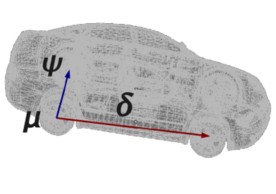
(a) Pose representation $\boldsymbol{\theta}$

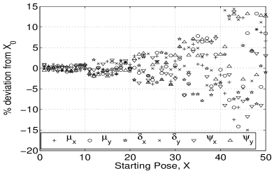
(b) Pose deviations

Figure 1: Figure 1(a) shows the pose representation $\boldsymbol{\theta}$ used for 3D car models. We use the rear wheel center $\boldsymbol{\mu}$, the vector between the wheel centres $\boldsymbol{\delta}$ and unit vector $\boldsymbol{\psi}$ in the direction of the rear wheel axle. Figure 1(b) shows the deviations of the randomly generated starting poses used for reliability testing. The test cases were generated to fall within percentage deviations in the ranges of 1%, 2%, 4%, 8% and 16% from the true pose $\boldsymbol{\theta}_{0}$ in the image. Poses 1-10 have a deviations of 1%, poses 11-20 have a deviation of 2% etc.

Artificial photographs. To understand the behaviour of the loss function, we have generated loss landscapes for artificial images of 3D models. To produce these landscapes, an artificial photograph was generated by projecting the 3D model at a known pose $\boldsymbol{\theta}_{0}$ with Phong shading. We then vary the pose parameters, two at a time about $\boldsymbol{\theta}_{0}$ and find the value of the loss function between this altered projection and the “photograph” taken at $\boldsymbol{\theta}_{0}$. These loss values are recorded, allowing us to visualise the behaviour of the loss function by observing surface and contour plots of these values. The unaltered pose values should project an image identical to the input photograph, giving a loss of zero according to the loss function derived in Section 4, with a higher loss exhibited at other poses. The variation of the loss with respect to a pair of pose parameters is shown in Figure 2(a). It can be seen from these loss landscapes that the loss has a clear minimum at the initial pose $\boldsymbol{\theta}_{0}$. The loss values increase as these pose parameters deviate away from $\boldsymbol{\theta}_{0}$, up to $\pm 20\%$. From this data, we are able to see that the minimum corresponding to $\boldsymbol{\theta}_{0}$ can be considered a global minimum for all practical purposes. The shape of the surface plots was similar for all other parameter pairs, indicating that the full 6D landscape of the loss function should similarly have a global minimum at the initial pose, allowing us to find this point using standard optimisation techniques, as demonstrated in Section 6.

Loss landscape. The landscape of the loss function was analysed for real photographs by varying the pose parameters of the model about a pose obtained by manually matching the 3D car model to a real photograph. The variation was plotted by taking a pair of pose parameters at a time over the entire set of pose parameters. A loss landscape obtained by varying $\mu_{y}$ and $\delta_{x}$ for a real photograph is shown in Figure 2(b). The variation of the loss function for other pose parameter pairs were found to be similar. Although a global minimum exists at the best pose of the real photograph, the nature of the loss function surface makes it more difficult to optimise when compared to artificial photos (Figure 2(a)). In particular, one can observe local minima in the periphery of the landscape, and the full 6D landscape is considerably more complex.

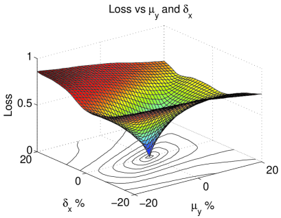
(a) Artificial photo

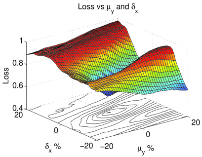
(b) Real photo

Figure 2: Loss landscapes for artificial and real photos. The six dimensional loss function was visualised by plotting its variation with a pair of pose parameters at a time. Based on our pose representation this results in fifteen plots. The variation of the loss function with a pair of pose parameters are shown for an artificial photograph and a real photograph. The nature of the loss function for real photographs makes it more difficult to find the global minimum (hence the correct pose) than for artificial photographs.

6 Optimising Vehicle Pose using the Loss Function

As explained in Section 4, the correct pose parameters $\boldsymbol{\theta_{opt}}$ will give the lowest loss value. The loss function landscape, as discussed in Section 5, shows that $\boldsymbol{\theta_{opt}}$ corresponds to the global minimum of the loss function. Therefore, an optimisation was performed on the loss function to obtain $\boldsymbol{\theta_{opt}}$ based on the pose representation $\boldsymbol{\theta}$ (Equation 5). The optimisation strategy and its reliability in different scenarios is discussed in this section.

The Optimiser. To immunise the optimisation from pixel quantisation artefacts and noise in the images, direct search methods that do not calculate the derivative of the loss function were considered. The optimisation was performed using the well known Downhill Simplex Method (DS) [NM65, PTVF07, Mat], owing to its efficiency and robustness. When optimising an $n$-dimensional function with the DS method, a so called simplex consisting of $n+1$ points is used to traverse the $n$-dimensional search space and find the optimum.

The reliability of the optimisation is adversely affected by the existence of local minima. Fortunately, the Downhill Simplex method has a useful property. In most cases, if the simplex is reinitialised at the pose parameters of the local minimum and the optimisation is performed again, the solution converges to the global minimum. Proper parameterisation is important for the optimiser to give good results. We have used a normalised pose parameterisation as follows.

Normalised pose parameters. Normalisation gives each pose parameter a comparable range during optimisation. The normalised pose $\boldsymbol{\boldsymbol{\theta}_{N}}$ was obtained by normalising $\boldsymbol{\mu}$ and $\boldsymbol{\delta}$ w.r.t. the dimensions of the photograph.

$$\boldsymbol{\boldsymbol{\theta}_{N}}=\left(\frac{\mu_{x}}{I_{W}},\frac{\mu_{y}}{I_{H}},\frac{\delta_{x}}{I_{W}},\frac{\delta_{y}}{I_{H}},\psi_{x},\psi_{y}\right)$$

$I_{W},I_{H}$ are the width and height of the photograph (2D image). $\boldsymbol{\psi}$ is a unit vector and does not require normalisation.

Initialisation. The downhill simplex method, like all optimisation techniques, requires a reasonable starting position. There are many methods for selecting a starting point, from repeated random initialisation to structured partitioning of the optimisation volume. A disadvantage of these methods is that they require a number of optimisation runs to locate the optimal point, which can take significant time. Depending on the application, it may be possible to develop a coarse location method which provides an estimate of the optimal pose.

The wheel match method described by Hutter and Brewer [HB09] is one such method, providing an initial match for a vehicle pose if the vehicle’s wheels are visible. Wheel match estimations using this method generally locate the wheel centres with a high degree of accuracy, but perform less effectively when determining the axle direction. This indicates that it may be possible to perform staged optimisation, attempting to fix some parameters before others. In general, parameter estimation using this method is within 5-15% of the true value. This initial pose selection is sufficient for our purposes.

Reliability of the pose estimate. Tests were carried out to asses the reliability of the pose estimate. We first generated synthetic “photographs” by rendering a 2D projection of a 3D car model at a known pose $\boldsymbol{\boldsymbol{\theta}_{0}}$. The optimisation was performed from initial poses $\boldsymbol{\boldsymbol{\theta}}$ that had a known deviation from $\boldsymbol{\boldsymbol{\theta}_{0}}$. Test poses were selected at 1%, 2%, 4%, 8% and 16% deviation from the known initial parameters so as to investigate a large hyper-volume in 6D space. The parameter values for 50 such random starting poses, 10 for each range, are shown in Figure  1(b). The reliability for each percentage range was defined as the proportion of correct matches in that deviation range. Exact pose recovery for synthetic images and better than careful manual tuning for real photos were regarded as correct. With this definition, a reliability of 1 indicates that all test cases in the range converged. A reliability of 0 indicates that none of the test cases in the range converged.

Reliability for artificial images. To ensure that the selected optimisation method is appropriate, we first investigate a simple case in which an artificial image with known parameters is constructed and used to validate the optimisation method. The reliability of the optimisation (with simplex re-initialisations) was found to be 100% (Figure 4) for initial poses with up to a 16% deviation from the matching pose.

Reliability for artificial images with real backgrounds. Next we rendered artificial car models on a real background photo, and performed the same reliability tests. Allowing simplex re-initialisations preserved a 100% convergence up to the 8% deviation range (Figure 4), although the simplex did not converge for certain starting poses at a 16% deviation. This shows that the effects of a real background can deteriorate the reliability of the pose estimate for higher deviations. In order to address this issue, a further refinement of the algorithm was made by clipping the background in the photograph when calculating the loss.

Clipping the background. The methodology used to lower the effects of the image background is as follows: Pixels in the projected image that do not correspond to points of the 3D model were treated as background. These pixels do not have surface normal components as they do not belong to the 3D model. Therefore, they can easily be filtered out by identifying pixels in the projected image that have null values for all three components $(x,y,z)$ of the surface normal. Only the remaining pixels $P=\{p\in Z\mskip-3.0mu\mskip-3.0mu\mskip-3.0muZ_{n_{x}}\times Z\mskip-3.0mu\mskip-3.0mu\mskip-3.0muZ_{n_{y}}:\boldsymbol{\phi}(p)\neq\boldsymbol{0}\}$ were considered for the loss calculation (Figure 4).

Reliability for real images using parallel projection. The reliability of the pose estimates on a real car photo are shown in Figure 4. Correct pose estimates with a high reliability were obtained for starting poses up to an 8% deviation.

Reliability for real images using perspective projection. The distance from the camera to the projection plane in the OpenGL perspective projection model was used as a seventh parameter when optimising using perspective projection. The extra pose parameter makes the optimisation harder at higher deviations as seen in the reliability graph in Figure 4. The reliability of the pose estimate may be further improved by using more sophisticated optimisation methods.

An example of a correctly estimated pose for a starting pose within a 16% deviation from the manually matched pose is shown in Figures 3(a) and 3(b). Given that we lack an absolute ground truth estimate, pose estimates were labelled as correct or incorrect based on their visual similarity to the input image.

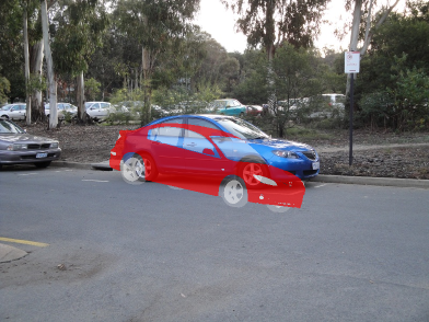
(a) Starting pose

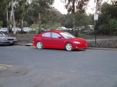
(b) Estimated pose

Figure 3: Pose estimation results. We show a sample pose estimation result for a real photograph of a 2005 Mazda 3 car. The car in the original photograph is blue. The estimated pose is shown by projecting the 3D car model over the photograph. The 3D car model is in red.

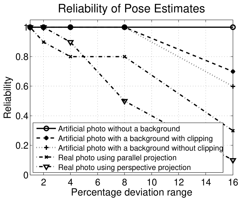
Figure 4: Results of the reliability tests. The graph shows the results of the reliability tests based on initial poses with percentage deviations as shown in Fig.1(b). Results for an artificial photograph (a projection of the 3D model), an artificial photograph with a real background superimposed and a real photograph are included.

7 Technical Aspects

In this section we describe some of the technical aspects of the proposed work. The initial code was implemented in MATLAB [Mat], however, components were gradually ported to C in order to improve performance.

3D rendering. In order to calculate the loss values described in Section 4, it was required to render the surface normals and brightness of a 3D model at a given pose. Initially, the rendering was done using model3D [Mic], a BSD licensed MATLAB [Mat] class. As this rendering was not fast enough for our application, a separate module was written in C to render the model off-screen using OpenGL [Ope] pBuffer extension and GLX. This C module was used with the MATLAB code using the MEX gateway. Initially, only the rendering was done in C. The rendered 2D intensity and surface normal matrices were returned back to MATLAB using the MEX gateway. This seemed to exhaust memory during the reliability tests described in Section 6. Therefore, the rendering and the loss calculation were also implemented in C, with only the loss value returned to MATLAB for use in optimisation.

Table 1: Rendering and loss calculation times.

Approach	Loss calc.	Render
MATLAB	0.16 s	2.28 s
C/OpenGL	0.04 s	0.17 s

This second approach improved performance in terms of speed and memory usage. A summary of the time taken to render the image and to calculate the loss using these approaches are presented in Table 1.

3D models. Triangulated 3D car models of significant complexity and detail in the AutoDesk 3DS file format were used for the work in this paper. These models were purchased from online 3D model vendors and had in the order of 30,000 nodes and in the order of 50,000 triangles.

Running times. A typical Downhill Simplex minimisation required in the order of 100–200 loss function evaluations. Using the C based loss calculation and OpenGL rendering, pose estimation in artificial images took around 1 minute for models with more than 30,000 nodes. Recent work done in [MNLF] on pose estimation using point correspondences, takes more than 3 minutes (200 seconds) for an artificial image of a model with only 80 points. Hence, despite being a pixel based method, the performance of our approach is very encouraging.

Possible improvements. The OpenGL context needs to be initialised each time the loss is calculated, when the C module (MEX) to calculate the loss is invoked from MATLAB. A further speed-up could be obtained by implementing the entire code (rendering and optimisation) in C, whereby the time spent on initialising the OpenGL context could be saved, as this needs to be done only once. It was also noted that although hardware accelerated OpenGL performs fast rendering, reading the rendered pixels back to main memory causes a performance bottleneck. The loss calculation may also be done in the graphics hardware itself, using GLSL or GPU computing, in order to avoid this bottleneck.

8 Discussion

Summary. A method to register a known 3D model on a given 2D image is presented in this paper. The correlation between attributes in the 2D image and projected 3D model are analysed in order to arrive at a correct pose estimate. The method differs from existing 2D-3D registration methods found in the literature. The proposed method requires only a single view of the object. It does not require a motion sequence and works on a static image from a given view. Also, the method does not require the camera parameters to be known a priori. Explicit point correspondences or matched features (which are hard to obtain when comparing 3D models and image modalities) need not be known beforehand. The method can recover the full 3D pose of an object. It does not require prior training or learning. As the method can handle 3D models of high complexity and detail, it could be used for applications that require detailed analysis of 2D images. It is particularly useful in situations where a known 3D model is used as a ground truth for analysing a 2D photograph. The method has been currently tested on real and artificial photographs of cars with promising results.

Outlook. A planned application of the method is to analyse images of damaged cars. A known 3D model of the damaged car will be registered on the image to be analysed, using the proposed registration method. This will be used as a ground truth. The method could be extended further to simultaneously identify the type of the car while estimating its pose, by optimising the loss function for a number of 3D models and selecting the model with the lowest loss value. More sophisticated optimisation methods may be used to improve results further.

Conclusion. We conclude from our results that the linearly invariant loss function derived in Section 4 can be used to estimate the pose of cars from real photographs. We also demonstrate that the Downhill Simplex method can be effectively used to optimise the loss function in order to obtain the correct pose. Allowing simplex re-initialisations makes the method more robust against local minima. The possibility of needing such re-initialisations can be significantly reduced by clipping the background of the image when calculating the loss. Despite being a direct pixel based method (as opposed to a feature/point based method), the performance of our method is very encouraging in comparison with other recent approaches, as discussed in Section 7.

References

- [ANB09] M. Arie-Nachimson and R. Basri. Constructing implicit 3d shape models for pose estimation. In ICCV, 2009.
- [Bro81] Brooks, R. A., and Binford, T. O. Geometric modelling in vision for manufacturing. In Proceedings of the Society of Photo-Optical Instrumentation Engineers Conference on Robot Vision, volume 281, pages 141–159, Washington, DC, USA, April 1981.
- [CD86] Roland T. Chin and Charles R. Dyer. Model-based recognition in robot vision. ACM Comput. Surv., 18(1):67–108, 1986.
- [DDDS04] P. David, D. DeMenthon, R. Duraiswami, and H. Samet. SoftPOSIT: Simultaneous pose and correspondence determination. International Journal of Computer Vision, 59(3):259–284, 2004.
- [DF90] R. Deriche and O. Faugeras. Tracking line segments. Image and Vision Computing, 8(4):261–270, 1990.
- [FP02] David A. Forsyth and Jean Ponce. Computer Vision: A Modern Approach. Prentice Hall Professional Technical Reference, 2002.
- [FvDFH95] J. D. Foley, A. v. Dam, S. K. Feiner, and J. F. Hughes. Computer Graphics: Principles and Practice in C. 2nd edition, 1995.
- [GA79] G. J. Gleason and G. J. Agin. A modular system for sensor-controlled manipulation and inspection. In Proceedings of the 9th International Symposium on Industrial Robots, pages 57–70, Washington, DC, USA, March 1979. Society of Manufacturing Engineers.
- [HB09] M. Hutter and N. Brewer. Matching 2-D Ellipses to 3-D Circles with Application to Vehicle Pose Identification. pages 153–158. Image and Vision Computing New Zealand, 2009. IVCNZ’09. 24th International Conference, 2009.
- [Hor75] B.K.P. Horn. Obtaining shape from shading information. In PsychCV75, pages 115–155, 1975.
- [HU90] D.P. Huttenlocher and S. Ullman. Recognizing solid objects by alignment with an image. International Journal of Computer Vision, 5(2):195–212, 1990.
- [KN97] Henner Kollnig and Hans-Hellmut Nagel. 3d pose estimation by directly matching polyhedral models to gray value gradients. Int. J. Comput. Vision, 23(3):283–302, 1997.
- [Mat] The MathWorks. MATLAB R2009b. http://www.mathworks.com.
-
[Mic]
Steven Michael.
Model3d.
http://www.mathworks.com/matlabcentral/fileexchange/7940-model3d. - [MNLF] F. Moreno-Noguer, V. Lepetit, and P. Fua. Pose priors for simultaneously solving alignment and correspondence. Computer Vision–ECCV 2008, pages 405–418.
- [NM65] JA Nelder and R. Mead. A simplex method for function minimization. The computer journal, 7(4):308, 1965.
- [Ope] OpenGL. http://www.opengl.org.
- [Per78] W. A. Perkins. A model-based vision system for industrial parts. IEEE Trans. Comput., 27(2):126–143, 1978.
- [Poj82] Poje, J. F., and Delp, E. J. A review of techniques for obtaining depth information with applications to machine vision. Technical report, Center for Robotics and Integrated Manufacturing, Univ. of Michigan, Ann Arbor, 1982.
- [PTVF07] William H. Press, Saul A. Teukolsky, William T. Vetterling, and Brian P. Flannery. Numerical recipes in C (3rd ed.): the art of scientific computing. Cambridge University Press, New York, NY, USA, 2007.
- [TB00] T.N. Tan and K.D. Baker. Efficient image gradient based vehicle localization. IEEE Transactions on Image Processing, 9(8):1343–1356, 2000.
- [Woo78] RJ Woodham. Photometric stereo: A reflectance map technique for determining surface orientation from image intensity. In Proc. SPIE, volume 155, pages 136–143, 1978.
- [XNJR03] E.P. Xing, A.Y. Ng, M.I. Jordan, and S. Russell. Distance metric learning with application to clustering with side-information. Advances in neural information processing systems, pages 521–528, 2003.
- [YT77] M. Yachida and S. Tsuji. A versatile machine vision system for complex industrial parts. IEEE Trans. Comput., 26(9):882–894, 1977.