Financial correlations at ultra-high frequency: theoretical models and empirical estimation

Iacopo Mastromatteo Iacopo Mastromatteo
SISSA, Via Beirut 2-4, 34014 Trieste, Italy
Matteo Marsili Matteo Marsili
The Abdus Salam International Centre for Theoretical Physics, Strada Costiera 11, 34014 Trieste, Italy
 and  Patrick Zoi Patrick Zoi
Risk & Capital Management, Assicurazioni Generali, Piazza Duca degli Abruzzi 2, 34132 Trieste, Italy
Abstract.

A detailed analysis of correlation between stock returns at high frequency is compared with simple models of random walks. We focus in particular on the dependence of correlations on time scales – the so-called Epps effect. This provides a characterization of stochastic models of stock price returns which is appropriate at very high frequency.

1. Introduction

The study of covariances between stocks is a central problem in finance, both to achieve theoretical understanding of market structure [1] and to exploit its relevant applications, such as portfolio optimization [2]. With the availability of financial high frequency data, it has become possible to estimate correlations on very short time scales, down to the frequency of individual transactions. As Epps first observed in 1979, the measured correlations between stock prices decrease as sampling frequency of time series grows [3]. Since then other studies on data coming from different stock markets [4] [5] and foreign exchange markets [6] [7] evidenced the persistence of such phenomenon – called Epps effects – across different markets.

Understanding the dependence of financial correlations on time scale has important practical consequences for portfolio management. For example, for large portfolios, the estimation of risk measures at low frequency (e.g. one day) suffers from instabilities, due to the scarcity of data [8]. Estimates of financial correlations – and hence of risk measures – at high frequency can rely on much richer and longer time series and can potentially detect structural changes more efficiently. Relating the structure of correlations at longer time scales to that at shorter time scales, provides means of overcoming the information deficiency causing the instability of risk measures. Interestingly, Borghesi et al. [9] found that the structure of correlations in groups of very liquid stocks, is largely invariant across time scales ranging from 5 minutes to one day. This suggests that estimates of correlations on long time scales from high frequency correlations is in principle feasible.

Transactions in financial markets play two rôles: in principle (i) they impact returns causing price movements, but in practice (ii) they also allow prices to be known, fixing the market value of a traded security until the next trade takes place. Correspondingly, two main contributions to the Epps effect have been considered in the literature so far: the first relates the Epps effect to genuine lagged correlations, and it arises from (temporary or permanent) impact of individual trades on the price dynamics. The second relates to the fact that price dynamics is not synchronous across stocks (i.e. transactions take place at different times, in principle, on different stocks).111The finiteness of the tick-size is also a significant source of Epps effect; its impact has been investigated in [10] [11].

Both lagged correlations and asynchronous sampling contribute to the Epps effect, but the relative weight of these two effects is not always easy to assess (see [12] and [13]): the first aspect to be considered is the fact that trading is not synchronous so that covariance estimation is intrinsically problematic at high frequency [14]. Lo and MacKinley proposed a solution to this issue based on a ”random censorship” model [15], which was able to explain why simple estimators tend to bias correlations towards zero at high frequency (more recent works following this line are [16] [17] [18] and [19]). The second factor contributing to the Epps effect is the presence of genuinely lagged correlations (lead-lag effect) [20] [21] [22], which should contain informations about the dynamical structure of the market.

This paper addresses the issue of disentangling these effects at very high frequency. We adopt an approach similar to [15], and use a previous tick estimator (see [23] for an analysis of interpolation-based estimators) to check the impact of asynchronous trading on correlations, without any specific choice for their genuine structure; alternative choices to deal with asynchrony are indeed available (namely [24] and [25]). The performance of some popular estimators has been investigated in [26].

We discuss a minimal model of price dynamics, which describes an infinitely liquid market: a transaction in this scenario has the only effect of revealing the asset price at a given instant of time, but sampling has no impact on prices. We find that also in this oversimplified scenario transactions can strongly affect correlations; in particular the Epps effect is always dominated by the asynchronous sampling at very high frequency. We show that it is possible to infer the genuine correlation structure of the market if one supposes inter-trade times to be exponentially distributed; in particular we can analytically disentangle the contribution to the Epps effect due to asynchronous trading to the one due to a genuine lag.

We apply the model to data of NYSE, finding that some features of the time series of returns at very high frequency can successfully be reproduced. In particular, assuming a process of asynchronous sampling of correlated random walks, we can estimate the underlying correlation function. The heterogeneity of sampling frequency in the bare data implies some predictability of less active stocks from the knowledge of more active ones. But once the effect of asynchronous sampling is removed, we find no causal structure in lagged cross-correlations. Still, cross-correlations are significantly non-zero over time lags of the order of ten seconds, whereas auto-correlations decay on the scale of one or two seconds. This provides evidence of an information contagion process across stocks, at ultra-high frequency.

The rest of the paper is organized as follows: we first discuss the origin of the Epps effect in simple theoretical models with synchronous (Section 2) or asynchronous sampling (Section 3). Section 4 discusses how to reconstruct the underlying correlations from asynchronously sampled data, in theoretical models. Section 5 applies these insights to empirical tick-by-tick data of NYSE. We summarize and discuss our results in Section 6. Technical derivations and proofs are relegated to the appendix for the sake of readability.

2. The origin of Epps effect: simple theoretical models

Consider a multivariate time series with stationary increments dXti𝑑subscriptsuperscript𝑋𝑖𝑡dX^{i}_{t}, where t𝑡t is a continuous time parameter and i=1,,n𝑖1𝑛i=1,\dots,n. The series will represent in the following the infinitesimal increment of the log-price of asset i𝑖i at time t𝑡t; let the finite variation of log-price after a time ΔtΔ𝑡\Delta t be given by222All the following considerations can be easily generalized to the discrete time case. We choose for simplicity to present them in continuous time. Notice that cτijsubscriptsuperscript𝑐𝑖𝑗𝜏c^{ij}_{\tau} is to be interpreted as a distribution (e.g. it may contain terms proportional to δ(τ)𝛿𝜏\delta(\tau)). :

XΔti=0Δt𝑑Xti,subscriptsuperscript𝑋𝑖Δ𝑡superscriptsubscript0Δ𝑡differential-dsubscriptsuperscript𝑋𝑖𝑡X^{i}_{\Delta t}=\int_{0}^{\Delta t}dX^{i}_{t}\;,

and say that the infinitesimal, lagged correlations are given by:

cttijdtdt=dXtidXtjsubscriptsuperscript𝑐𝑖𝑗𝑡superscript𝑡𝑑𝑡𝑑superscript𝑡delimited-⟨⟩𝑑subscriptsuperscript𝑋𝑖𝑡𝑑subscriptsuperscript𝑋𝑗superscript𝑡c^{ij}_{t-t^{\prime}}\,dt\,dt^{\prime}=\langle dX^{i}_{t}dX^{j}_{t^{\prime}}\rangle

while the spectrum Sωijsubscriptsuperscript𝑆𝑖𝑗𝜔S^{ij}_{\omega} is defined as

Sωij=+𝑑τcτijeiωτ.subscriptsuperscript𝑆𝑖𝑗𝜔superscriptsubscriptdifferential-d𝜏subscriptsuperscript𝑐𝑖𝑗𝜏superscript𝑒𝑖𝜔𝜏S^{ij}_{\omega}=\int_{-\infty}^{+\infty}d\tau\,c^{ij}_{\tau}\,e^{i\omega\tau}.

We will be interested in characterizing the dependence of the finite, equal time correlation CΔtij=XΔtiXΔtjsubscriptsuperscript𝐶𝑖𝑗Δ𝑡delimited-⟨⟩subscriptsuperscript𝑋𝑖Δ𝑡subscriptsuperscript𝑋𝑗Δ𝑡C^{ij}_{\Delta t}=\langle X^{i}_{\Delta t}X^{j}_{\Delta t}\rangle on the time scale ΔtΔ𝑡\Delta t. Its behavior can be extracted from the knowledge of the series dXti𝑑subscriptsuperscript𝑋𝑖𝑡dX^{i}_{t}, which can be related to CΔtijsubscriptsuperscript𝐶𝑖𝑗Δ𝑡C^{ij}_{\Delta t} as:

CΔtijsubscriptsuperscript𝐶𝑖𝑗Δ𝑡\displaystyle C^{ij}_{\Delta t} =\displaystyle= 0Δt0Δt𝑑t𝑑tcttijsuperscriptsubscript0Δ𝑡superscriptsubscript0Δ𝑡differential-d𝑡differential-dsuperscript𝑡subscriptsuperscript𝑐𝑖𝑗𝑡superscript𝑡\displaystyle\int_{0}^{\Delta t}\int_{0}^{\Delta t}dt\,dt^{\prime}\,c^{ij}_{t-t^{\prime}}
=\displaystyle= 12π+𝑑ωSωijω2(eiωΔt1)(eiωΔt1)12𝜋superscriptsubscriptdifferential-d𝜔subscriptsuperscript𝑆𝑖𝑗𝜔superscript𝜔2superscript𝑒𝑖𝜔Δ𝑡1superscript𝑒𝑖𝜔Δ𝑡1\displaystyle\frac{1}{2\pi}\int_{-\infty}^{+\infty}d\omega\,\frac{S^{ij}_{\omega}}{\omega^{2}}\left(e^{-i\omega\Delta t}-1\right)\left(e^{i\omega\Delta t}-1\right)

While for a purely Brownian motion, the scaling of CΔtijsubscriptsuperscript𝐶𝑖𝑗Δ𝑡C^{ij}_{\Delta t} is linear in ΔtΔ𝑡\Delta t, in the general case we will quantify deviations from linearity of CΔtijsubscriptsuperscript𝐶𝑖𝑗Δ𝑡C^{ij}_{\Delta t} by considering the quantity:

(2) ρΔtij=CΔtijCΔtiiCΔtjj,subscriptsuperscript𝜌𝑖𝑗Δ𝑡subscriptsuperscript𝐶𝑖𝑗Δ𝑡subscriptsuperscript𝐶𝑖𝑖Δ𝑡subscriptsuperscript𝐶𝑗𝑗Δ𝑡\rho^{ij}_{\Delta t}=\frac{C^{ij}_{\Delta t}}{\sqrt{C^{ii}_{\Delta t}C^{jj}_{\Delta t}}}\;,

that is the Pearson correlation coefficient, built by normalizing the covariance to the variances. We will say that the Epps effect is absent whenever ρΔtijsubscriptsuperscript𝜌𝑖𝑗Δ𝑡\rho^{ij}_{\Delta t} is independent of ΔtΔ𝑡\Delta t, and it is present otherwise.

It is interesting to remark some general features of ρΔtijsubscriptsuperscript𝜌𝑖𝑗Δ𝑡\rho^{ij}_{\Delta t}: first, the positivity of the eigenvalues of the covariance matrix CΔtijsubscriptsuperscript𝐶𝑖𝑗Δ𝑡C^{ij}_{\Delta t} ensures that |ρΔtij|1subscriptsuperscript𝜌𝑖𝑗Δ𝑡1|\rho^{ij}_{\Delta t}|\leq 1. The finiteness of the limit Δt0Δ𝑡0\Delta t\rightarrow 0 of ρΔtijsubscriptsuperscript𝜌𝑖𝑗Δ𝑡\rho^{ij}_{\Delta t} can then be checked from the continuity of the coefficients: if both auto- and cross-correlations are infinite at the origin, then ρΔtijsubscriptsuperscript𝜌𝑖𝑗Δ𝑡\rho^{ij}_{\Delta t} is finite; the same holds if auto- and cross-correlations are both finite at the origin. The case with infinite auto-correlations and finite cross-correlations gives instead ρΔtij0subscriptsuperscript𝜌𝑖𝑗Δ𝑡0\rho^{ij}_{\Delta t}\rightarrow 0: whenever the time needed by the system to auto-correlate is much smaller than the time needed to cross-correlate, then the equal time correlation coefficient goes to 0. In the opposite limit ΔtΔ𝑡\Delta t\rightarrow\infty, if +𝑑τcτij=𝒞ijsuperscriptsubscriptdifferential-d𝜏subscriptsuperscript𝑐𝑖𝑗𝜏superscript𝒞𝑖𝑗\int_{-\infty}^{+\infty}d\tau\,c^{ij}_{\tau}=\mathcal{C}^{ij} is finite, one can also see that:

ρij=𝒞ij𝒞ii𝒞jjsubscriptsuperscript𝜌𝑖𝑗superscript𝒞𝑖𝑗superscript𝒞𝑖𝑖superscript𝒞𝑗𝑗\rho^{ij}_{\infty}=\frac{\mathcal{C}^{ij}}{\sqrt{\mathcal{C}^{ii}\mathcal{C}^{jj}}}

The behavior of ρΔtijsubscriptsuperscript𝜌𝑖𝑗Δ𝑡\rho^{ij}_{\Delta t} during the transient is also interesting, as it contains non-trivial informations about the time needed by the system to correlate the dynamics. The origin of the Epps effect is best illustrated by discussing few simple examples.

2.1. Example (Correlated Brownian motions):

Let’s consider the case of a bivariate process of the kind:

dXt1𝑑subscriptsuperscript𝑋1𝑡\displaystyle dX^{1}_{t} =\displaystyle= cdηt0+1cdηt1𝑐𝑑subscriptsuperscript𝜂0𝑡1𝑐𝑑subscriptsuperscript𝜂1𝑡\displaystyle\sqrt{c}\,d\eta^{0}_{t}+\sqrt{1-c}\,d\eta^{1}_{t}
dXt2𝑑subscriptsuperscript𝑋2𝑡\displaystyle dX^{2}_{t} =\displaystyle= cdηt0+1cdηt2𝑐𝑑subscriptsuperscript𝜂0𝑡1𝑐𝑑subscriptsuperscript𝜂2𝑡\displaystyle\sqrt{c}\,d\eta^{0}_{t}+\sqrt{1-c}\,d\eta^{2}_{t}

where the dηti𝑑superscriptsubscript𝜂𝑡𝑖d\eta_{t}^{i} are white noises, so that dηtidηtj=delimited-⟨⟩𝑑superscriptsubscript𝜂𝑡𝑖𝑑subscriptsuperscript𝜂𝑗superscript𝑡absent\langle d\eta_{t}^{i}d\eta^{j}_{t^{\prime}}\rangle=
δijδttdtdtsuperscript𝛿𝑖𝑗subscript𝛿𝑡superscript𝑡𝑑𝑡𝑑superscript𝑡\delta^{ij}\delta_{t-t^{\prime}}\,dt\,dt^{\prime}. Then this is the only case in which linearity strictly holds both for variance and covariance:

CΔt12subscriptsuperscript𝐶12Δ𝑡\displaystyle C^{12}_{\Delta t} =\displaystyle= cΔt𝑐Δ𝑡\displaystyle c\,\Delta t
CΔtiisubscriptsuperscript𝐶𝑖𝑖Δ𝑡\displaystyle C^{ii}_{\Delta t} =\displaystyle= ΔtΔ𝑡\displaystyle\phantom{c\,}\Delta t

so that:

ρΔt12=c,subscriptsuperscript𝜌12Δ𝑡𝑐\rho^{12}_{\Delta t}=c\;,

independent of ΔtΔ𝑡\Delta t, and there is no Epps effect.

2.2. Example (Lagged series):

Let’s now consider the lagged version of the previous process:

dXt1𝑑subscriptsuperscript𝑋1𝑡\displaystyle dX^{1}_{t} =\displaystyle= cdηt0+1cdηt1𝑐𝑑subscriptsuperscript𝜂0𝑡1𝑐𝑑subscriptsuperscript𝜂1𝑡\displaystyle\sqrt{c}\,d\eta^{0}_{t\phantom{+\tau}}+\sqrt{1-c}\,d\eta^{1}_{t}
dXt2𝑑subscriptsuperscript𝑋2𝑡\displaystyle dX^{2}_{t} =\displaystyle= cdηt+τ0+1cdηt2𝑐𝑑subscriptsuperscript𝜂0𝑡𝜏1𝑐𝑑subscriptsuperscript𝜂2𝑡\displaystyle\sqrt{c}\,d\eta^{0}_{t+\tau}+\sqrt{1-c}\,d\eta^{2}_{t}

In this case:

cttiisuperscriptsubscript𝑐𝑡superscript𝑡𝑖𝑖\displaystyle c_{t-t^{\prime}}^{ii} =\displaystyle= δttsubscript𝛿𝑡superscript𝑡\displaystyle\phantom{c}\,\delta_{t-t^{\prime}}
ctt12superscriptsubscript𝑐𝑡superscript𝑡12\displaystyle c_{t-t^{\prime}}^{12} =\displaystyle= cδttτ𝑐subscript𝛿𝑡superscript𝑡𝜏\displaystyle c\,\delta_{t-t^{\prime}-\tau}

and it is easy to see (appendix B) that ρ𝜌\rho results in this case:

ρΔt12=c(1τΔt)θ(Δtτ),subscriptsuperscript𝜌12Δ𝑡𝑐1𝜏Δ𝑡𝜃Δ𝑡𝜏\rho^{12}_{\Delta t}=c\left(1-\frac{\tau}{\Delta t}\right)\theta(\Delta t-\tau)\;,

where θ(t)𝜃𝑡\theta(t) is the step function, so the presence of an Epps effect is evident.

2.3. Example (Different widths):

We can now consider another bivariate process, whose lagged correlations are:

ctt12superscriptsubscript𝑐𝑡superscript𝑡12\displaystyle c_{t-t^{\prime}}^{12} =\displaystyle= c(12ξle|tt|/ξl)𝑐12subscript𝜉𝑙superscript𝑒𝑡superscript𝑡subscript𝜉𝑙\displaystyle c\,\left(\frac{1}{2\,\xi_{l}}e^{-|t-t^{\prime}|/\xi_{l}}\right)
cttiisuperscriptsubscript𝑐𝑡superscript𝑡𝑖𝑖\displaystyle c_{t-t^{\prime}}^{ii} =\displaystyle= 12ξse|tt|/ξs,12subscript𝜉𝑠superscript𝑒𝑡superscript𝑡subscript𝜉𝑠\displaystyle\phantom{c\,(}\frac{1}{2\,\xi_{s}}e^{-|t-t^{\prime}|/\xi_{s}}\,,

with the conditions ξlξssubscript𝜉𝑙subscript𝜉𝑠\xi_{l}\geq\xi_{s} and c1𝑐1c\leq 1 ensuring |ρΔt12|1subscriptsuperscript𝜌12Δ𝑡1|\rho^{12}_{\Delta t}|\leq 1. In this case one has:

ρΔt12=c[Δt+ξl(eΔt/ξl1)Δt+ξs(eΔt/ξs1)]subscriptsuperscript𝜌12Δ𝑡𝑐delimited-[]Δ𝑡subscript𝜉𝑙superscript𝑒Δ𝑡subscript𝜉𝑙1Δ𝑡subscript𝜉𝑠superscript𝑒Δ𝑡subscript𝜉𝑠1\rho^{12}_{\Delta t}=c\left[\frac{\Delta t+\xi_{l}\left(e^{-\Delta t/\xi_{l}}-1\right)}{\Delta t+\xi_{s}\left(e^{-\Delta t/\xi_{s}}-1\right)}\right]

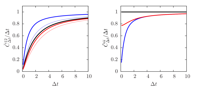
Such quantity is a constant only for ξs=ξlsubscript𝜉𝑠subscript𝜉𝑙\xi_{s}=\xi_{l}, while in the general case it is a function which grows from ρ012=cξs/ξlsubscriptsuperscript𝜌120𝑐subscript𝜉𝑠subscript𝜉𝑙\rho^{12}_{0}=c\,\xi_{s}/\xi_{l} to an asymptotic value ρ12subscriptsuperscript𝜌12\rho^{12}_{\infty}, as represented in the blue lines of figure 3. The case ξs0subscript𝜉𝑠0\xi_{s}\rightarrow 0 is also interesting, as the variance becomes linear, while ρΔtijsubscriptsuperscript𝜌𝑖𝑗Δ𝑡\rho^{ij}_{\Delta t} is given by:

ρΔt12=c[1+ξlΔt(eΔt/ξl1)]subscriptsuperscript𝜌12Δ𝑡𝑐delimited-[]1subscript𝜉𝑙Δ𝑡superscript𝑒Δ𝑡subscript𝜉𝑙1\rho^{12}_{\Delta t}=c\left[1+\frac{\xi_{l}}{\Delta t}\left(e^{-\Delta t/\xi_{l}}-1\right)\right]

The above examples show that an Epps effect is present if the covariance of a process grows with ΔtΔ𝑡\Delta t at a rate smaller than the variance, or equivalently the infinitesimal, lagged cross-correlations cτijsubscriptsuperscript𝑐𝑖𝑗𝜏c^{ij}_{\tau} are not proportional to auto-correlations cτiisubscriptsuperscript𝑐𝑖𝑖𝜏c^{ii}_{\tau}. We will see in section 5 that financial time series show at high frequency a correlation structure which is reminiscent of the one of these examples; in particular such structure is well fitted by a model where the dynamics of correlations is described by a lag parameter τ𝜏\tau and a width parameter ξ𝜉\xi, and where variances grow faster with respect to covariances. In [27] this approach is also used to describe the dynamics related with the time evolution of the correlation matrix.

3. Asynchronous sampling of correlated random walks

While studying a multivariate time series at very high frequency (say, tick-by-tick financial data), it is unlikely that all transactions happen simultaneously; additionally some time bin may contain no data point at all, as no transaction took place. This fact may cause problems in the estimation of volatilities and correlations [14], especially in the extreme case in which one tries to evaluate such quantities at time scales of the order of the inter-trade time. A possible approach to deal with this issue is the creation of a synchronous series [15] out of the asynchronous one by means of some prescription, such as linear interpolation or previous-tick interpolation [23]. We adopt this latter, simpler estimator to study the impact of asynchrony on measured correlations, as it allows an easy analytical treatment of such quantities without requiring any assumption on their genuine nature (in particular we will focus on models containing lagged and short ranged correlations).

Consider an underlying synchronous process dXti𝑑subscriptsuperscript𝑋𝑖𝑡dX^{i}_{t} defined as in section 2, and n𝑛n subsets of points Ui={tki}ksuperscript𝑈𝑖subscriptsubscriptsuperscript𝑡𝑖𝑘𝑘U^{i}=\{t^{i}_{k}\}_{k\in\mathbb{Z}} randomly drawn on the real line. Let the probability of drawing a point between t𝑡t and t+dt𝑡𝑑𝑡t+dt for subset Uisuperscript𝑈𝑖U^{i} be given by λidtsubscript𝜆𝑖𝑑𝑡\lambda_{i}\,dt. In this way for each subset Uisuperscript𝑈𝑖U^{i} the number of points drawn in an interval [t1,t2]subscript𝑡1subscript𝑡2[t_{1},t_{2}] is a Poissonian random variable of mean λi(t2t1)subscript𝜆𝑖subscript𝑡2subscript𝑡1\lambda_{i}\,(t_{2}-t_{1}). The corresponding waiting time distribution is exponential, and is given by pi(t)=λieλitsubscript𝑝𝑖𝑡subscript𝜆𝑖superscript𝑒subscript𝜆𝑖𝑡p_{i}(t)=\lambda_{i}e^{-\lambda_{i}t}. Given a set of Uisuperscript𝑈𝑖U^{i} and a realization of the underlying synchronous process Xtisubscriptsuperscript𝑋𝑖𝑡X^{i}_{t}, one can define an asynchronous process:

X~Δti=t1t2𝑑Xtisubscriptsuperscript~𝑋𝑖Δ𝑡superscriptsubscriptsubscript𝑡1subscript𝑡2differential-dsubscriptsuperscript𝑋𝑖𝑡\tilde{X}^{i}_{\Delta t}=\int_{t_{1}}^{t_{2}}dX^{i}_{t}

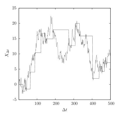
where t1=max{tkiUi|tki<0}subscript𝑡1subscriptsuperscript𝑡𝑖𝑘conditionalsuperscript𝑈𝑖subscriptsuperscript𝑡𝑖𝑘0t_{1}=\max\{t^{i}_{k}\in U^{i}|\,t^{i}_{k}<0\} and t2=max{tkiUi|tki<Δt}subscript𝑡2subscriptsuperscript𝑡𝑖𝑘conditionalsuperscript𝑈𝑖subscriptsuperscript𝑡𝑖𝑘Δ𝑡t_{2}=\max\{t^{i}_{k}\in U^{i}|\,t^{i}_{k}<\Delta t\}. This time series is a piecewise constant function, with discrete jumps at the points Δt=tkiΔ𝑡subscriptsuperscript𝑡𝑖𝑘\Delta t=t^{i}_{k} , as shown in figure 1); notice that this construction implements the previous tick estimator prescription (PTE) to deal with missing data.
Refer to caption
Figure 1. We plot here a realization of a synchronous process XΔtsubscript𝑋Δ𝑡X_{\Delta t} (dashed line), and a randomly sampled version of the same realization (full line), obtained with a sampling rate λ=0.05𝜆0.05\lambda=0.05.

Covariance can be defined in this case as:

C~Δtij=E[X~ΔtiX~Δtj]subscriptsuperscript~𝐶𝑖𝑗Δ𝑡𝐸delimited-[]delimited-⟨⟩subscriptsuperscript~𝑋𝑖Δ𝑡subscriptsuperscript~𝑋𝑗Δ𝑡\tilde{C}^{ij}_{\Delta t}=E\left[\langle\tilde{X}^{i}_{\Delta t}\tilde{X}^{j}_{\Delta t}\rangle\right]

where E[]𝐸delimited-[]E[\cdot] denotes expectation value with respect to the sampling process. Then one can generalize the Epps effect, defining as in the previous case the function ρ~Δtijsubscriptsuperscript~𝜌𝑖𝑗Δ𝑡\tilde{\rho}^{ij}_{\Delta t}: if such function depends on ΔtΔ𝑡\Delta t, (generalized) Epps effect is present, otherwise it is absent.

We will now show three properties which allow to extract information about the asynchronous process X~Δtisubscriptsuperscript~𝑋𝑖Δ𝑡\tilde{X}^{i}_{\Delta t} given the spectrum of the synchronous process XΔtisubscriptsuperscript𝑋𝑖Δ𝑡X^{i}_{\Delta t}. The proof of these results is given in appendix A.

P1: Covariance of asynchronous processes

Given an asynchronous time series X~Δtisuperscriptsubscript~𝑋Δ𝑡𝑖\tilde{X}_{\Delta t}^{i} defined using a synchronous time series of spectrum Sωijsubscriptsuperscript𝑆𝑖𝑗𝜔S^{ij}_{\omega} and waiting time distributions pi(t)=θ(t)λieλitsuperscript𝑝𝑖𝑡𝜃𝑡subscript𝜆𝑖superscript𝑒subscript𝜆𝑖𝑡p^{i}(t)=\theta(t)\lambda_{i}\,e^{-\lambda_{i}t}, for ij𝑖𝑗i\neq j it holds:

(3) C~Δtij=12π+𝑑ωSωijω2[λiλj(λi+iω)(λjiω)](eiωΔt1)(eiωΔt1)subscriptsuperscript~𝐶𝑖𝑗Δ𝑡12𝜋superscriptsubscriptdifferential-d𝜔subscriptsuperscript𝑆𝑖𝑗𝜔superscript𝜔2delimited-[]subscript𝜆𝑖subscript𝜆𝑗subscript𝜆𝑖𝑖𝜔subscript𝜆𝑗𝑖𝜔superscript𝑒𝑖𝜔Δ𝑡1superscript𝑒𝑖𝜔Δ𝑡1\tilde{C}^{ij}_{\Delta t}=\frac{1}{2\pi}\int_{-\infty}^{+\infty}d\omega\,\frac{S^{ij}_{\omega}}{\omega^{2}}\,\left[\frac{\lambda_{i}\lambda_{j}}{(\lambda_{i}+i\omega)(\lambda_{j}-i\omega)}\right]\left(e^{-i\omega\Delta t}-1\right)\left(e^{i\omega\Delta t}-1\right)

Equivalently, covariance in the asynchronous case can be computed by correcting the synchronous spectrum with the substitution:

(4) S~ωij=Sωijλiλj(λi+iω)(λjiω)subscriptsuperscript~𝑆𝑖𝑗𝜔subscriptsuperscript𝑆𝑖𝑗𝜔subscript𝜆𝑖subscript𝜆𝑗subscript𝜆𝑖𝑖𝜔subscript𝜆𝑗𝑖𝜔\tilde{S}^{ij}_{\omega}=S^{ij}_{\omega}\frac{\lambda_{i}\lambda_{j}}{(\lambda_{i}+i\omega)(\lambda_{j}-i\omega)}

In real space, such substitution is equivalent to the convolution:

(5) c~ttij=λiλj(λi+λj)[t𝑑τctτijeλj(tτ)+t+𝑑τctτijeλi(τt)].superscriptsubscript~𝑐𝑡superscript𝑡𝑖𝑗subscript𝜆𝑖subscript𝜆𝑗subscript𝜆𝑖subscript𝜆𝑗delimited-[]superscriptsubscriptsuperscript𝑡differential-d𝜏superscriptsubscript𝑐𝑡𝜏𝑖𝑗superscript𝑒subscript𝜆𝑗superscript𝑡𝜏superscriptsubscriptsuperscript𝑡differential-d𝜏superscriptsubscript𝑐𝑡𝜏𝑖𝑗superscript𝑒subscript𝜆𝑖𝜏superscript𝑡\tilde{c}_{t-t^{\prime}}^{ij}=\frac{\lambda_{i}\lambda_{j}}{(\lambda_{i}+\lambda_{j})}\Bigg{[}\int_{-\infty}^{t^{\prime}}d\tau\;c_{t-\tau}^{ij}e^{-\lambda_{j}(t^{\prime}-\tau)}+\int_{t^{\prime}}^{+\infty}d\tau\;c_{t-\tau}^{ij}e^{-\lambda_{i}(\tau-t^{\prime})}\Bigg{]}.

P2: Variance of asynchronous processes

Consider the asynchronous time series X~Δtsubscript~𝑋Δ𝑡\tilde{X}_{\Delta t}, defined using a synchronous time series of spectrum Sωsubscript𝑆𝜔S_{\omega} and a waiting time distribution p(t)=θ(t)λeλt𝑝𝑡𝜃𝑡𝜆superscript𝑒𝜆𝑡p(t)=\theta(t)\lambda\,e^{-\lambda t}. Then it holds:

C~Δtsubscript~𝐶Δ𝑡\displaystyle\tilde{C}_{\Delta t} =\displaystyle= 12π+𝑑ωSωω2(eiωΔt1)(eiωΔt1)+limit-from12𝜋superscriptsubscriptdifferential-d𝜔subscript𝑆𝜔superscript𝜔2superscript𝑒𝑖𝜔Δ𝑡1superscript𝑒𝑖𝜔Δ𝑡1\displaystyle\frac{1}{2\pi}\int_{-\infty}^{+\infty}d\omega\,\frac{S_{\omega}}{\omega^{2}}\left(e^{-i\omega\Delta t}-1\right)\left(e^{i\omega\Delta t}-1\right)+
+\displaystyle+ 2λ2[12π+𝑑ωSω1+ω2/λ2(eiωΔteλΔt)]2superscript𝜆2delimited-[]12𝜋superscriptsubscriptdifferential-d𝜔subscript𝑆𝜔1superscript𝜔2superscript𝜆2superscript𝑒𝑖𝜔Δ𝑡superscript𝑒𝜆Δ𝑡\displaystyle\frac{2}{\lambda^{2}}\left[\frac{1}{2\pi}\int_{-\infty}^{+\infty}d\omega\,\frac{S_{\omega}}{1+\omega^{2}/\lambda^{2}}\left(e^{-i\omega\Delta t}-e^{-\lambda\Delta t}\right)\right]

Equivalently, to compute the variance in the asynchronous case it is necessary to add to the synchronous value a correction, so that one gets:

(6) C~Δt=CΔt+2λ2(c¯ΔteλΔtc¯0)subscript~𝐶Δ𝑡subscript𝐶Δ𝑡2superscript𝜆2subscript¯𝑐Δ𝑡superscript𝑒𝜆Δ𝑡subscript¯𝑐0\tilde{C}_{\Delta t}=C_{\Delta t}+\frac{2}{\lambda^{2}}\left(\bar{c}_{\Delta t}-e^{-\lambda\Delta t}\bar{c}_{0}\right)\,

where c¯τsubscript¯𝑐𝜏\bar{c}_{\tau} is the Fourier anti-transform of the damped spectrum Sω1+ω2/λ2subscript𝑆𝜔1superscript𝜔2superscript𝜆2\frac{S_{\omega}}{1+\omega^{2}/\lambda^{2}}.

P3: Case of linear variance

If an asynchronous time series X~Δtsubscript~𝑋Δ𝑡\tilde{X}_{\Delta t} is defined using a synchronous series of variance CΔtsubscript𝐶Δ𝑡C_{\Delta t} linear in ΔtΔ𝑡\Delta t (corresponding to a constant spectrum Sωsubscript𝑆𝜔S_{\omega}) and waiting time distribution p(t)=θ(t)λeλt𝑝𝑡𝜃𝑡𝜆superscript𝑒𝜆𝑡p(t)=\theta(t)\lambda\,e^{-\lambda t}, then the asynchronous value of its variance corresponds to the synchronous one.

The property P1 shows what is the effect of the random sampling on the measured covariance: if λ=λi=λj𝜆subscript𝜆𝑖subscript𝜆𝑗\lambda=\lambda_{i}=\lambda_{j} substitution (4) is a low-pass filter (a Lorentzian) with a cutoff scale set by λ𝜆\lambda, which suppresses signal at frequencies bigger than the sampling scale. In the case λiλjsubscript𝜆𝑖subscript𝜆𝑗\lambda_{i}\neq\lambda_{j} an effect of spurious causality333We employ the term ”causality” in a loose sense, using the expression ”returns of stock i𝑖i cause returns of stock j𝑗j” to signify that cτij>cτijsubscriptsuperscript𝑐𝑖𝑗𝜏subscriptsuperscript𝑐𝑖𝑗𝜏c^{ij}_{\tau}>c^{ij}_{-\tau}, that is, an asymmetry is measured in the lagged correlation of two stocks is also induced: kernel (4) has in general a complex phase, which generates an asymmetry between c~τijsubscriptsuperscript~𝑐𝑖𝑗𝜏\tilde{c}^{ij}_{\tau} and c~τijsubscriptsuperscript~𝑐𝑖𝑗𝜏\tilde{c}^{ij}_{-\tau}, as pointed out in [15]. The direction of such asymmetry is such that the more frequently sampled series appears to influence the less sampled one: this merely reflects the fact that one can use the information contained in the more sampled series to successfully forecast the less sampled one. The property P2 allows to calculate in general the asynchronous value of the variance, and in particular for the simple case of a very narrow correlation coefficient cτiisubscriptsuperscript𝑐𝑖𝑖𝜏c^{ii}_{\tau} P3 implies that variance doesn’t necessarily decrease as λisubscript𝜆𝑖\lambda_{i} gets smaller, while covariance always gets suppressed; this is why, generally speaking, asynchronous sampling tends to enhance Epps effect. Notice that, while P1 directly relates cτijsubscriptsuperscript𝑐𝑖𝑗𝜏c^{ij}_{\tau} with c~τijsubscriptsuperscript~𝑐𝑖𝑗𝜏\tilde{c}^{ij}_{\tau} (and Sωijsubscriptsuperscript𝑆𝑖𝑗𝜔S^{ij}_{\omega} with S~ωijsubscriptsuperscript~𝑆𝑖𝑗𝜔\tilde{S}^{ij}_{\omega}), P2 just connects CΔtiisubscriptsuperscript𝐶𝑖𝑖Δ𝑡C^{ii}_{\Delta t} with C~Δtiisubscriptsuperscript~𝐶𝑖𝑖Δ𝑡\tilde{C}^{ii}_{\Delta t}: the asynchronous value of the auto-correlation function c~τiisubscriptsuperscript~𝑐𝑖𝑖𝜏\tilde{c}^{ii}_{\tau} has to be indirectly obtained from C~Δtiisubscriptsuperscript~𝐶𝑖𝑖Δ𝑡\tilde{C}^{ii}_{\Delta t}. For τ0𝜏0\tau\neq 0, this can be done by observing that:

(7) d2dΔt2C~Δtii|Δt=τ=c~τii+c~τii=2c~τii=1π𝑑ωS~ωiieiωτevaluated-atsuperscript𝑑2𝑑Δsuperscript𝑡2subscriptsuperscript~𝐶𝑖𝑖Δ𝑡Δ𝑡𝜏superscriptsubscript~𝑐𝜏𝑖𝑖superscriptsubscript~𝑐𝜏𝑖𝑖2subscriptsuperscript~𝑐𝑖𝑖𝜏1𝜋differential-d𝜔subscriptsuperscript~𝑆𝑖𝑖𝜔superscript𝑒𝑖𝜔𝜏\frac{d^{2}}{d\Delta t^{2}}\tilde{C}^{ii}_{\Delta t}\Bigg{|}_{\Delta t=\tau}=\tilde{c}_{\tau}^{ii}+\tilde{c}_{-\tau}^{ii}=2\tilde{c}^{ii}_{\tau}=\frac{1}{\pi}\int d\omega\,\tilde{S}^{ii}_{\omega}\,e^{-i\omega\tau}

For τ=0𝜏0\tau=0 instead the auto-correlation c~τiisubscriptsuperscript~𝑐𝑖𝑖𝜏\tilde{c}^{ii}_{\tau} may contain a δτsubscript𝛿𝜏\delta_{\tau}, which can be deduced from the behavior of C~Δtiisubscriptsuperscript~𝐶𝑖𝑖Δ𝑡\tilde{C}^{ii}_{\Delta t} for Δt0Δ𝑡0\Delta t\rightarrow 0. Specifically, if C~ΔtiiΔtsimilar-tosubscriptsuperscript~𝐶𝑖𝑖Δ𝑡Δ𝑡\tilde{C}^{ii}_{\Delta t}\sim\Delta t, then the auto-correlation is divergent in τ=0𝜏0\tau=0, which signals the presence of a term δτsubscript𝛿𝜏\delta_{\tau}. Conversely, if C~ΔtiiΔt2similar-tosubscriptsuperscript~𝐶𝑖𝑖Δ𝑡Δsuperscript𝑡2\tilde{C}^{ii}_{\Delta t}\sim\Delta t^{2} or if C~Δtiisubscriptsuperscript~𝐶𝑖𝑖Δ𝑡\tilde{C}^{ii}_{\Delta t} vanishes faster than Δt2Δsuperscript𝑡2\Delta t^{2}, then c~τiisuperscriptsubscript~𝑐𝜏𝑖𝑖\tilde{c}_{\tau}^{ii} is regular in 0.

These results allow us to generalize the analysis of the examples in section 2 to the asynchronous case.

3.1. Example (Correlated Brownian motions):

In this simple case the synchronous value of the correlation coefficient is given by:

cτ12=cδτsuperscriptsubscript𝑐𝜏12𝑐subscript𝛿𝜏c_{\tau}^{12}=c\,\delta_{\tau}\,

If now we suppose the rates of the sampling processes to be all equal to λ𝜆\lambda, equation (5) can be used to calculate the asynchronous value of covariance, while the variance inherits linearity from the synchronous case. The result reads (see appendix B):

ρ~Δt12=c(1+1λΔt(eλΔt1)),subscriptsuperscript~𝜌12Δ𝑡𝑐11𝜆Δ𝑡superscript𝑒𝜆Δ𝑡1\tilde{\rho}^{12}_{\Delta t}=c\,\left(1+\frac{1}{\lambda\Delta t}\left(e^{-\lambda\Delta t}-1\right)\right)\;,

which is plotted in figure 3 (black line). In this case we have a spurious (induced by the sampling) Epps effect, as the original time series did not show any Epps effect.

3.2. Example (Lagged series):

Now we turn to the synchronous process:

dXt1𝑑subscriptsuperscript𝑋1𝑡\displaystyle dX^{1}_{t} =\displaystyle= cdηt0+1cdηt1𝑐𝑑subscriptsuperscript𝜂0𝑡1𝑐𝑑subscriptsuperscript𝜂1𝑡\displaystyle\sqrt{c}\,d\eta^{0}_{t\phantom{+\tau}}+\sqrt{1-c}\,d\eta^{1}_{t}
dXt2𝑑subscriptsuperscript𝑋2𝑡\displaystyle dX^{2}_{t} =\displaystyle= cdηt+τ0+1cdηt2𝑐𝑑subscriptsuperscript𝜂0𝑡𝜏1𝑐𝑑subscriptsuperscript𝜂2𝑡\displaystyle\sqrt{c}\,d\eta^{0}_{t+\tau}+\sqrt{1-c}\,d\eta^{2}_{t}

and consider again sampling rates λ1=λ2=λsubscript𝜆1subscript𝜆2𝜆\lambda_{1}=\lambda_{2}=\lambda. Then, using the above properties, one can find that (see appendix B):

ρ~Δtij={c2λΔteλ(Δt+τ)(1eλΔt)2ifΔt<τcλΔt[eλΔtcosh(λτ)eλτ]+c(1τΔt)ifΔt>τsubscriptsuperscript~𝜌𝑖𝑗Δ𝑡cases𝑐2𝜆Δ𝑡superscript𝑒𝜆Δ𝑡𝜏superscript1superscript𝑒𝜆Δ𝑡2ifΔ𝑡𝜏missing-subexpressionmissing-subexpressionmissing-subexpressionlimit-from𝑐𝜆Δ𝑡delimited-[]superscript𝑒𝜆Δ𝑡𝜆𝜏superscript𝑒𝜆𝜏missing-subexpressionmissing-subexpressionmissing-subexpressionmissing-subexpressionmissing-subexpression𝑐1𝜏Δ𝑡ifΔ𝑡𝜏\tilde{\rho}^{ij}_{\Delta t}=\left\{\begin{array}[]{lcc}\displaystyle{\frac{c}{2\lambda\Delta t}e^{-\lambda(\Delta t+\tau)}\left(1-e^{\lambda\Delta t}\right)^{2}}&\rm{if}&\Delta t<\tau\\ \phantom{,}&&\\ \displaystyle{\frac{c}{\lambda\Delta t}\left[e^{-\lambda\Delta t}\cosh(\lambda\tau)-e^{-\lambda\tau}\right]+}&&\\ \\ \displaystyle{c\left(1-\frac{\tau}{\Delta t}\right)}&\rm{if}&\Delta t>\tau\end{array}\right.

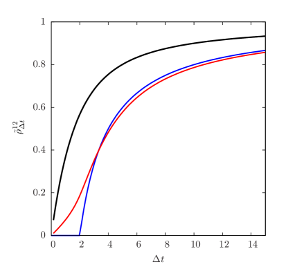
and check that Epps effect is enhanced by the effect of the sampling (covariance grows even slower than in the synchronous case), so that genuine and spurious effects superimpose as shown in figure 2.
Refer to caption
Figure 2. Equal time correlation coefficient for two lagged processes, both for the case of synchronous and asynchronous sampling. The lag parameter τ𝜏\tau and the sampling rate λ𝜆\lambda are set to τ=0,λ=1formulae-sequence𝜏0𝜆1\tau=0,\lambda=1 (black line), τ=2,λ=formulae-sequence𝜏2𝜆\tau=2,\lambda=\infty (blue), τ=2,λ=1formulae-sequence𝜏2𝜆1\tau=2,\lambda=1 (red line).

3.3. Example (Different widths):

Also in this case the genuine Epps effect is enhanced by the asynchronous sampling; indeed in this case both variance and covariance are influenced by the sampling and produce a spurious effect. It is possible to calculate the coefficient C~Δt12subscriptsuperscript~𝐶12Δ𝑡\tilde{C}^{12}_{\Delta t} assuming sampling rates λ1subscript𝜆1\lambda_{1} and λ2subscript𝜆2\lambda_{2}. Its value reads:

C~Δt12=c[Δt+(λ1λ2ξl32u1v2(eΔt/ξl1)λ2λ1(λ1+λ2)u1v1(eλ1Δt1))+(λ1λ2)]\tilde{C}^{12}_{\Delta t}=c\,\Bigg{[}\Delta t+\bigg{(}\frac{\lambda_{1}\lambda_{2}\xi_{l}^{3}}{2u_{1}v_{2}}(e^{-\Delta t/\xi_{l}}-1)-\frac{\lambda_{2}}{\lambda_{1}(\lambda_{1}+\lambda_{2})u_{1}v_{1}}(e^{-\lambda_{1}\Delta t}-1)\bigg{)}+\bigg{(}\lambda_{1}\leftrightarrow\lambda_{2}\bigg{)}\Bigg{]}

where the coefficients uisubscript𝑢𝑖u_{i} and visubscript𝑣𝑖v_{i} are defined in appendix B. The variance is given by:

C~Δtii=Δt+ξs(λi2ξs2(eΔt/ξs1)(eλiΔt1)λi2ξs21)subscriptsuperscript~𝐶𝑖𝑖Δ𝑡Δ𝑡subscript𝜉𝑠superscriptsubscript𝜆𝑖2superscriptsubscript𝜉𝑠2superscript𝑒Δ𝑡subscript𝜉𝑠1superscript𝑒subscript𝜆𝑖Δ𝑡1superscriptsubscript𝜆𝑖2superscriptsubscript𝜉𝑠21\tilde{C}^{ii}_{\Delta t}=\Delta t+\xi_{s}\left(\frac{\lambda_{i}^{2}\xi_{s}^{2}(e^{-\Delta t/\xi_{s}}-1)-(e^{-\lambda_{i}\Delta t}-1)}{\lambda_{i}^{2}\xi_{s}^{2}-1}\right)

Notice that the sampling induces a singular auto-correlation function for the variance: while the synchronous value of cτiisubscriptsuperscript𝑐𝑖𝑖𝜏c^{ii}_{\tau} is regular in the origin, one can check that it becomes singular in zero as an effect of the sampling. In particular, using equation (7), one finds that the asynchronous auto-correlation is given by:

c~τii=11+λiξsδτ+ξsλi22(λi2ξs21)(e|τ|/ξeλi|τ|),subscriptsuperscript~𝑐𝑖𝑖𝜏11subscript𝜆𝑖subscript𝜉𝑠subscript𝛿𝜏subscript𝜉𝑠superscriptsubscript𝜆𝑖22superscriptsubscript𝜆𝑖2superscriptsubscript𝜉𝑠21superscript𝑒𝜏𝜉superscript𝑒subscript𝜆𝑖𝜏\tilde{c}^{ii}_{\tau}=\frac{1}{1+\lambda_{i}\xi_{s}}\,\delta_{\tau}+\frac{\xi_{s}\lambda_{i}^{2}}{2(\lambda_{i}^{2}\xi_{s}^{2}-1)}\left(e^{-|\tau|/\xi}-e^{-\lambda_{i}|\tau|}\right)\;,

and it is easy to see that the regular part goes to zero for small values of τ𝜏\tau, a feature which is also present in empirical data.
This example shows how the Epps effect can be induced both from variance and covariance (as in this case neither of those quantities is linear), and that the sampling may additionally give a spurious contribution to the Epps effect (as the functional dependence of C~Δtijsubscriptsuperscript~𝐶𝑖𝑗Δ𝑡\tilde{C}^{ij}_{\Delta t} and C~Δtiisubscriptsuperscript~𝐶𝑖𝑖Δ𝑡\tilde{C}^{ii}_{\Delta t} changes due to the sampling). In figure 3 some typical curves for normalized variance and covariance are presented for this model.
Refer to caption
Figure 3. Normalized covariance and variance for two processes displaying exponential decay both of cross-correlation and of auto-correlation, where the decay constant are respectively ξlsubscript𝜉𝑙\xi_{l} and ξssubscript𝜉𝑠\xi_{s}, with ξs<ξlsubscript𝜉𝑠subscript𝜉𝑙\xi_{s}<\xi_{l}. Both the case of synchronous and asynchronous sampling (of common rate λ𝜆\lambda) are represented. On the right, the variance is plotted in the cases λ=𝜆\lambda=\infty, ξs=0.3subscript𝜉𝑠0.3\xi_{s}=0.3 (blue line), λ=1𝜆1\lambda=1, ξs=0subscript𝜉𝑠0\xi_{s}=0 (black line) and λ=1𝜆1\lambda=1, ξs=0.3subscript𝜉𝑠0.3\xi_{s}=0.3 (red line). On the left, the covariance is represented in the cases λ=𝜆\lambda=\infty, ξl=0.4subscript𝜉𝑙0.4\xi_{l}=0.4 (thick blue line), λ=𝜆\lambda=\infty, ξl=0.8subscript𝜉𝑙0.8\xi_{l}=0.8 (narrow blue line), λ=1𝜆1\lambda=1, ξl=0.4subscript𝜉𝑙0.4\xi_{l}=0.4 (thick red line), λ=1𝜆1\lambda=1, ξl=0.8subscript𝜉𝑙0.8\xi_{l}=0.8 (narrow red line) and λ=1𝜆1\lambda=1, ξl=0subscript𝜉𝑙0\xi_{l}=0 (black line).

4. Filtering of asynchronous time series

An interesting application of property (5) concerns data filtering of asynchronous time series: as it is possible to quantify how a synchronous time series is influenced by an exponential random sampling, it is also possible to discount its damping effect on the high frequency region of the cross-correlation spectrum. As the random sampling induces a convolution with a known kernel, the reconstruction of the genuine cross correlation structure requires a deconvolution. In particular, given a measured asynchronous time series X~tisubscriptsuperscript~𝑋𝑖𝑡\tilde{X}^{i}_{t}, the deconvolution procedure can be carried on following these lines:

  1. (1)

    Calculate the measured spectrum S~ωijsubscriptsuperscript~𝑆𝑖𝑗𝜔\tilde{S}^{ij}_{\omega} of the time series from raw data X~tisubscriptsuperscript~𝑋𝑖𝑡\tilde{X}^{i}_{t}

  2. (2)

    Compute the sampling rate λisubscript𝜆𝑖\lambda_{i} for each process;

  3. (3)

    Estimate the genuine spectrum S^ωijsuperscriptsubscript^𝑆𝜔𝑖𝑗\hat{S}_{\omega}^{ij}444Notice that the corrected spectrum has the right properties to construct consistent correlation matrices; in particular it is Hermitian and it satisfies S^ωji=S^ωijsubscriptsuperscript^𝑆𝑗𝑖𝜔subscriptsuperscript^𝑆𝑖𝑗𝜔\hat{S}^{ji}_{\omega}=\hat{S}^{ij}_{-\omega}. by inverting (4):

    S^ωij=S~ωij(λiλj(λi+iω)(λjiω))1=S~ωijKωij1superscriptsubscript^𝑆𝜔𝑖𝑗superscriptsubscript~𝑆𝜔𝑖𝑗superscriptsubscript𝜆𝑖subscript𝜆𝑗subscript𝜆𝑖𝑖𝜔subscript𝜆𝑗𝑖𝜔1superscriptsubscript~𝑆𝜔𝑖𝑗subscriptsuperscript𝐾𝑖𝑗1𝜔\hat{S}_{\omega}^{ij}=\tilde{S}_{\omega}^{ij}\left(\frac{\lambda_{i}\lambda_{j}}{(\lambda_{i}+i\omega)(\lambda_{j}-i\omega)}\right)^{-1}=\tilde{S}_{\omega}^{ij}K^{ij\,-1}_{\omega}
  4. (4)

    Write cross-correlations c^ttijsuperscriptsubscript^𝑐𝑡superscript𝑡𝑖𝑗\hat{c}_{t-t^{\prime}}^{ij} using equation (2)

This deconvolution procedure, known as inverse filtering, should in principle allow to compute the genuine signal with infinite accuracy; in practice, dealing with time series of finite length and in which time is discretized, some effects have to be taken into account. Moreover, while effects of discreteness and finite size are easy to quantify (appendix C), a more careful treatment of noise is needed: as the inverse deconvolution amplifies the high frequency region of the spectrum with a term proportional to ω2superscript𝜔2\omega^{2}, the noise that typically dominates that region affects crucially the accuracy of the reconstructed signal. A possible solution is to set a cutoff to the maximum frequency used to deconvolve the spectrum, choosing for example a deconvolution kernel of the kind:

S^ωij=S~ωijKωij1(|Kωij|2|Kωij|2+SNRω1ij)subscriptsuperscript^𝑆𝑖𝑗𝜔subscriptsuperscript~𝑆𝑖𝑗𝜔subscriptsuperscript𝐾𝑖𝑗1𝜔superscriptsubscriptsuperscript𝐾𝑖𝑗𝜔2superscriptsubscriptsuperscript𝐾𝑖𝑗𝜔2superscriptsubscriptSNR𝜔1𝑖𝑗\hat{S}^{ij}_{\omega}=\tilde{S}^{ij}_{\omega}K^{ij\,-1}_{\omega}\left(\frac{|K^{ij}_{\omega}|^{2}}{|K^{ij}_{\omega}|^{2}+{\rm SNR}_{\omega}^{-1\,ij}}\right)

where SNRωijsubscriptsuperscriptSNRij𝜔\rm{SNR}^{ij}_{\omega} is the expected signal-to-noise ratio of the genuine signal. This leads to what is called a Wiener filter [29].

5. Empirical analysis on NYSE data

An empirical analysis has been carried on using tick-by-tick data from the New York Stock Exchange (NYSE) collected during the period going from 02.01.2003 to
12.31.2003. We studied daily time series (T=20000𝑇20000T=20000 seconds) of the 100 most traded stocks, excluding for each day the first 45 and the last 21 minutes of trades, and then averaged over a set of M=248𝑀248M=248 days to obtain the spectra S~ωijsuperscriptsubscript~𝑆𝜔𝑖𝑗\tilde{S}_{\omega}^{ij}. X~Δtisubscriptsuperscript~𝑋𝑖Δ𝑡\tilde{X}^{i}_{\Delta t} was computed from the observed values of logptisuperscriptsubscript𝑝𝑡𝑖\log p_{t}^{i}, where the price was defined to be constant between consecutive trades (PTE prescription). All series have been normalized to zero mean and unit variance. It has been assumed that measured prices are randomly sampled points of an underlying synchronous time series as described above. The sampling rates λisubscript𝜆𝑖\lambda_{i} were computed for each stock and the waiting time distributions have been taken to be exponential as a first order approximation.

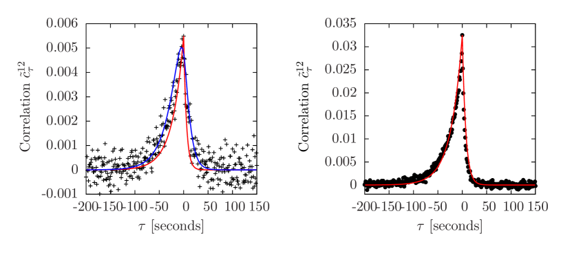
Cross-correlation coefficients have been systematically calculated; as expected raw cross-correlation coefficients c~τijsubscriptsuperscript~𝑐𝑖𝑗𝜏\tilde{c}^{ij}_{\tau} show a narrow peak near τ=0𝜏0\tau=0 corresponding to the market mode (figure 4), justifying a fit with functions of the form:

(8) c~τij=csynce|ττsync|/ξsyncsubscriptsuperscript~𝑐𝑖𝑗𝜏subscript𝑐𝑠𝑦𝑛𝑐superscript𝑒𝜏subscript𝜏𝑠𝑦𝑛𝑐subscript𝜉𝑠𝑦𝑛𝑐\tilde{c}^{ij}_{\tau}=c_{sync}\,e^{-|\tau-\tau_{sync}|/\xi_{sync}}
Refer to caption
Figure 4. Left: The raw, infinitesimal cross-correlation coefficient c~τGE/Ksubscriptsuperscript~𝑐𝐺𝐸𝐾𝜏\tilde{c}^{\,GE/K}_{\tau} is shown for the pair of assets GE and K as a function of the lag τ𝜏\tau (black points); the asymmetry of this function can be explained assuming genuine correlations of the simple form cτGE/K=cδτsubscriptsuperscript𝑐𝐺𝐸𝐾𝜏𝑐subscript𝛿𝜏c^{GE/K}_{\tau}=c\,\delta_{\tau} and convoluting the effect of the sampling (red line); the best fit of the form of equation (9) is also shown (blue line). Right: Infinitesimal cross-correlation coefficient c~τ12subscriptsuperscript~𝑐12𝜏\tilde{c}^{12}_{\tau} for two asynchronously sampled processes (black points); the evolution of the underlying time series with constant correlation was simulated. Sampling times were taken to coincide with those of the stocks GE and K in the data set. The red line shows the theoretical correlation curve obtained for the same underlying process with an exponential waiting time distribution matching the measured sampling rates.

The influence of the asynchronous sampling on these inferred parameters is indeed relevant, as the typical sampling times λ1superscript𝜆1\lambda^{-1} are of the same order of ξsyncsubscript𝜉𝑠𝑦𝑛𝑐\xi_{sync}; the simplest way to take into account its effect is to fit using functions of the form:

(9) c~τij=casyne|ττasyn|/ξasynKτijsubscriptsuperscript~𝑐𝑖𝑗𝜏subscript𝑐𝑎𝑠𝑦𝑛superscript𝑒𝜏subscript𝜏𝑎𝑠𝑦𝑛subscript𝜉𝑎𝑠𝑦𝑛subscriptsuperscript𝐾𝑖𝑗𝜏\tilde{c}^{ij}_{\tau}=c_{asyn}\,e^{-|\tau-\tau_{asyn}|/\xi_{asyn}}*K^{ij}_{\tau}

where Kτijsubscriptsuperscript𝐾𝑖𝑗𝜏K^{ij}_{\tau} is the kernel appearing in (5), which depends on the estimated sampling frequencies λisubscript𝜆𝑖\lambda_{i} and λjsubscript𝜆𝑗\lambda_{j}, and * denotes convolution.

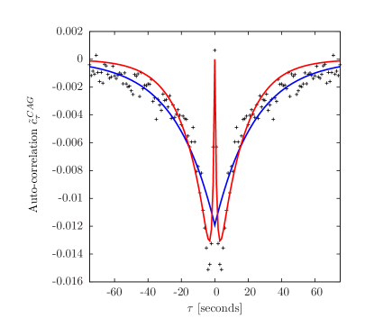
Auto-correlations have also been computed for all the stocks, and both their qualitative and quantitative behavior turn out to be very different from the case of cross-correlations. In particular one can see that all auto-correlations are positively divergent in the origin, but assume finite values for lags different than 0, as shown in figure 5. Then the simplest fit that can be performed is the one with a function of the kind:

(10) c~τii=asyncδτbsync(e|τ|/ξsync2ξsync)subscriptsuperscript~𝑐𝑖𝑖𝜏subscript𝑎𝑠𝑦𝑛𝑐subscript𝛿𝜏subscript𝑏𝑠𝑦𝑛𝑐superscript𝑒𝜏subscript𝜉𝑠𝑦𝑛𝑐2subscript𝜉𝑠𝑦𝑛𝑐\tilde{c}^{ii}_{\tau}=a_{sync}\,\delta_{\tau}-b_{sync}\left(\frac{e^{-|\tau|/\xi_{sync}}}{2\,\xi_{sync}}\right)

which is the superposition of a purely Brownian part with a fast decaying part. As in the case of cross-correlations, we can also fit those functions using their asynchronous counterpart:

c~τiisubscriptsuperscript~𝑐𝑖𝑖𝜏\displaystyle\tilde{c}^{ii}_{\tau} =\displaystyle= (aasynbasyn1+λiξasyn)δτsubscript𝑎𝑎𝑠𝑦𝑛subscript𝑏𝑎𝑠𝑦𝑛1subscript𝜆𝑖subscript𝜉𝑎𝑠𝑦𝑛subscript𝛿𝜏\displaystyle\left(a_{asyn}-\frac{b_{asyn}}{1+\lambda_{i}\xi_{asyn}}\right)\delta_{\tau}
\displaystyle- basyn[ξasynλi22[(λiξasyn)21](e|τ|/ξasyneλi|τ|)],subscript𝑏𝑎𝑠𝑦𝑛delimited-[]subscript𝜉𝑎𝑠𝑦𝑛superscriptsubscript𝜆𝑖22delimited-[]superscriptsubscript𝜆𝑖subscript𝜉𝑎𝑠𝑦𝑛21superscript𝑒𝜏subscript𝜉𝑎𝑠𝑦𝑛superscript𝑒subscript𝜆𝑖𝜏\displaystyle b_{asyn}\left[\frac{\xi_{asyn}\lambda_{i}^{2}}{2[(\lambda_{i}\xi_{asyn})^{2}-1]}\left(e^{-|\tau|/\xi_{asyn}}-e^{-\lambda_{i}|\tau|}\right)\right]\;,

as suggested by the examples discussed in the previous sections.
Refer to caption
Figure 5. A typical infinitesimal auto-correlation coefficient (in this case c~τCAGsubscriptsuperscript~𝑐𝐶𝐴𝐺𝜏\tilde{c}^{\,CAG}_{\tau}) is plotted (black points). Its best fit of the form (10) is plotted in blue, while the best fit of the form (5) is represented in red. Notice that even if the empirical function we plotted is negative and has a bimodal shape, a positive diverging contribution in τ=0𝜏0\tau=0 should also be taken into account.

The results of the fit of auto- and cross-correlation coefficient with the raw and corrected functions defined above are summarized in Table 1, where three kinds of ensembles (AC, T and L) were considered.

Table 1. Results for auto- and cross-correlation coefficients c~τijsubscriptsuperscript~𝑐𝑖𝑗𝜏\tilde{c}^{ij}_{\tau} fitted against the functions defined in section 5 for various ensembles. Ensemble AC, used to compute auto-correlations, contains the 100 most traded assets of the NYSE, while ensembles T and L contain, respectively, the 10 more traded and the 10 less traded assets of the same market, and have been used to compute cross-correlation functions. For each of the parameters we write the ensemble average and show in parenthesis its standard deviation.
Ensemble ξsyncsubscript𝜉𝑠𝑦𝑛𝑐\xi_{sync} ξasynsubscript𝜉𝑎𝑠𝑦𝑛\xi_{asyn} τsyncsubscript𝜏𝑠𝑦𝑛𝑐\tau_{sync} τasynsubscript𝜏𝑎𝑠𝑦𝑛\tau_{asyn} χsync2χasyn21subscriptsuperscript𝜒2𝑠𝑦𝑛𝑐subscriptsuperscript𝜒2𝑎𝑠𝑦𝑛1\frac{\chi^{2}_{sync}}{\chi^{2}_{asyn}}-1
AC 21.8 1.27  - - 0.30
(32.3) (1.36)  - - (0.63)0.63(0.63)
T-T 12.93 7.69 0.30 -0.27 -0.05
(1.56) (2.07) (1.55) (1.98) (0.14)
T-L 21.42 9.36 8.62 2.10 0.69
(3.99) (4.45) (4.62) (4.04) (0.36)
L-L 28.36 10.85 -0.73 -1.66 0.005
(4.60) (6.13) (4.14) (4.98) (0.08)0.08(0.08)

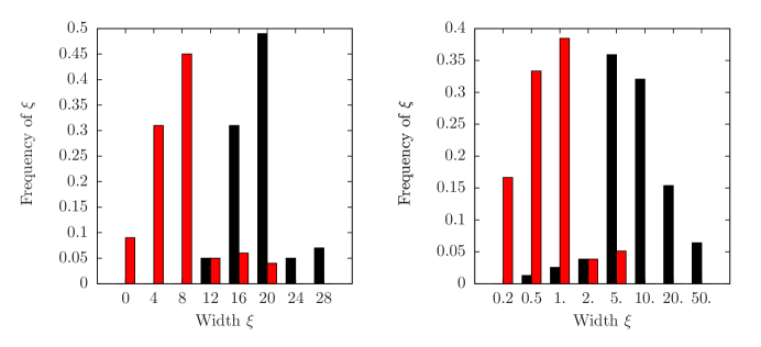
First we discuss the results for the ensemble AC, which contains the 100 most traded assets of NYSE, and has been used to compute the infinitesimal auto-correlation coefficients. The raw functions have a raw width ξsyncsubscript𝜉𝑠𝑦𝑛𝑐\xi_{sync} broadly distributed around a mean value of 20 s, as shown in Table 1, and are typically characterized by a bimodal shape (79% of the empirical functions are compatible with zero for τ=0𝜏0\tau=0) which the raw model cannot account for. The inclusion of the sampling effect in the fitting functions improves the descriptive power of the model just slightly: on average the chi-square is reduced of about 30%, but fluctuations in the ensemble are strong. Indeed, the asynchrony explains naturally the bimodal shape of the auto-correlations, and shifts the width of the corrected function ξasynsubscript𝜉𝑎𝑠𝑦𝑛\xi_{asyn} to a small interval centered around a value of 1 s (figure 6), providing thus a mechanism to explain most of the signal width. A similar result holds for the ratios async/bsyncsubscript𝑎𝑠𝑦𝑛𝑐subscript𝑏𝑠𝑦𝑛𝑐a_{sync}/b_{sync} and aasyn/basynsubscript𝑎𝑎𝑠𝑦𝑛subscript𝑏𝑎𝑠𝑦𝑛a_{asyn}/b_{asyn}: while the former follows a broad distribution, the latter is sharply peaked around a mean value of 1.5absent1.5\approx 1.5. These results do not qualitatively change if one takes as synchronous fitting function the superposition of a delta function with two exponentials.

The other ensembles which have been considered are T and L, containing respectively the 10 most and less traded assets of the AC ensemble; they have been used to calculate the infinitesimal cross-correlation coefficient for all the pairs of the form T-L, T-T and L-L. The inferred widths ξsyncsubscript𝜉𝑠𝑦𝑛𝑐\xi_{sync} are generally spread on a window of 30 s, ranging from 10 seconds (T-T ensemble) to 40 seconds (L-L), while the values of τsyncsubscript𝜏𝑠𝑦𝑛𝑐\tau_{sync} often exceed 10 s in the T-L case, indicating that a lack of symmetry is present in this ensemble; the direction of the asymmetry reveals an influence of the most traded stocks towards the less traded ones. For the T-L ensemble, the asynchronous model turns out to provide a better description of the data (see e.g. figure 4), as residuals are significantly reduced, and most of the asymmetry is accounted for in the kernel. Additionally, asynchronous sampling explains much of the observed width of correlations functions, as shown in figure 6. Still, compared to auto-correlations the histogram of estimated widths of cross-correlations is centered at values significantly different from zero, of the order of 10 seconds.
Refer to caption
Figure 6. Histogram of the fitted values of ξsyncsubscript𝜉𝑠𝑦𝑛𝑐\xi_{sync} (black bars) and ξasynsubscript𝜉𝑎𝑠𝑦𝑛\xi_{asyn} (red bars), both for cross-correlations (left) and auto-correlations (right). In the case of cross-correlations we considered a sample consisting of the 10 more active assets and the 10 less active ones, while for the auto-correlation we considered the 100 most active assets. Notice that while the left plot is in linear-linear scale, the right one is in log-linear scale: for auto-correlations most of the width is induced by the sampling, while for the cross-correlations the asynchrony seems to play a less significant rôle.

In the T-T and L-L cases the descriptive power of the two models is almost identical (when sampling rates are similar, it becomes harder to statistically discriminate functions (8) and (9)). Again, even if a part of the width ξsyncsubscript𝜉𝑠𝑦𝑛𝑐\xi_{sync} is explained by sampling, the value of ξasynsubscript𝜉𝑎𝑠𝑦𝑛\xi_{asyn} is significantly different from zero, meaning that other mechanisms contribute to the formation of Epps effect. Interestingly, while the raw width varies significantly within the ensembles T-L, T-T and L-L, the corrected width ξasynsubscript𝜉𝑎𝑠𝑦𝑛\xi_{asyn} is compatible for all of them and of the order of 10 seconds.

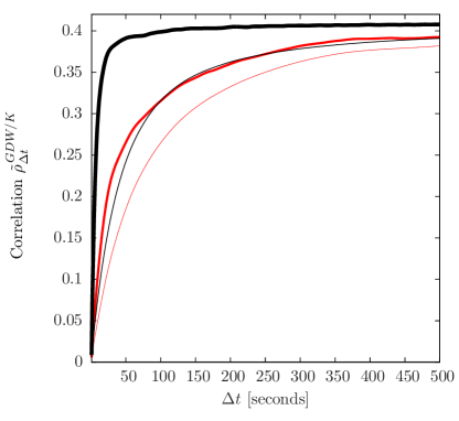
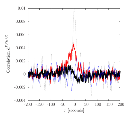
In order to compensate for the effect of the sampling it is also possible to filter the raw signal using the procedure described above; this allows us to evaluate the impact of the asynchrony on the measured correlations as a function of the scale ΔtΔ𝑡\Delta t. Figure 7 shows the saturation curves of the correlation ρΔtijsubscriptsuperscript𝜌𝑖𝑗Δ𝑡\rho^{ij}_{\Delta t} for a pair of assets using both raw and filtered data and compares them with the ones obtained for a pair of simulated Brownian motions with the same asymptotic value of correlation. Results obtained for simulated data set the maximum efficiency of the filter, which is fixed by the length of the time series; empirical data show that the reconstructed curve is well below such bound, indicating that other effects do contribute to the formation of the Epps. These features include by micro-structural effects, such as finite tick-size [10] [11], and possibly an intrinsic time scale related to human reaction [16] . The same features are detected in figure 8, where the infinitesimal, raw cross-correlations c~τijsubscriptsuperscript~𝑐𝑖𝑗𝜏\tilde{c}^{ij}_{\tau} are compared to the filtered ones; the presence of a residual Epps effect is indicated here by the finite width of the filtered curve. Additionally, most of the asymmetry contained in the raw curve can be successfully removed, as most of the lag is induced as an effect of the different sampling rates.
Refer to caption
Figure 7. The raw equal time correlation coefficient ρ~ΔtGDW/Ksubscriptsuperscript~𝜌𝐺𝐷𝑊𝐾Δ𝑡\tilde{\rho}^{\,GDW/K}_{\Delta t} (narrow red line) is shown for the pair GDW and K, together with the same curve obtained with filtered data (thick red line). The black line corresponds to the correlation coefficient for a simulated process with the same asymptotic value of ρ~Δt12subscriptsuperscript~𝜌12Δ𝑡\tilde{\rho}^{12}_{\Delta t}, sampling rates and statistics of the other curves, whose cross and auto-correlations are δτproportional-toabsentsubscript𝛿𝜏\propto\delta_{\tau}; the dashed line is the filtered version of the same curve.
Refer to caption
Figure 8. Raw and filtered infinitesimal cross-correlation coefficients c~τPFE/Ksubscriptsuperscript~𝑐𝑃𝐹𝐸𝐾𝜏\tilde{c}^{\,PFE/K}_{\tau} for stocks PFE and K calculated in year 2003 (respectively, red and dotted line), together with their asymmetrical parts (c~τPFE/Kc~τPFE/K)/2subscriptsuperscript~𝑐𝑃𝐹𝐸𝐾𝜏subscriptsuperscript~𝑐𝑃𝐹𝐸𝐾𝜏2(\tilde{c}^{\,PFE/K}_{\tau}-\tilde{c}^{\,PFE/K}_{-\tau})/2 (black and blue line).

Within this approach it is also necessary to estimate from empirical data the nature of the waiting time distribution, as it usually deviates from the exponential one which is assumed. The effect of the deviations must then be evaluated to ensure the consistency of the procedure previously described. We analyzed this issue by simulating a set of synchronous time series of known spectrum, and sampling them using points extracted from real data; then spectra for those series were systematically checked against the analytical predictions obtained for an exponential waiting time distribution. On the right side of figure 4 we compare the effect of an exponential sampling with the real one, finding that no significant difference is induced by fluctuations of λisubscript𝜆𝑖\lambda_{i}.

6. Conclusions

In this paper we investigated the time-dependence of financial correlations and their decay at very high frequency (Epps effect), showing that some simple models of stochastic process are able to describe this features. We found that in case of exponentially sampled data the impact of asynchrony on correlations can be analytically controlled, and its contribution can be exactly evaluated. We also find that within this framework one can successfully describe some features of the empirical correlations observed in the NYSE market, namely the heterogeneity of the price change predictability and the presence of a causal structure in the cross-correlations. The first feature is detected as a broad distribution of widths both in the auto- and cross-correlation functions of the assets, and can be explained by taking into account the effect of the sampling. The second one is quantified by the lag of cross-correlation functions, and again can be almost completely justified by including the sampling effect. Finally, we find that a significant fraction of the Epps effect cannot be explained as just due to the effect of asynchrony, indicating that other kind of effects, conjectured in [16] to be related to time scales of human reaction, contribute to the observed dynamics of correlations.

Appendix A Effect of an exponential random sampling

We now turn to prove the properties which allow us to analytically account for the effect of the random sampling.
To prove property P1, we consider a multivariate synchronous process XΔtisubscriptsuperscript𝑋𝑖Δ𝑡X^{i}_{\Delta t}, and let the asynchronous sampling be induced by a waiting time distribution pi(t)=λieλitsubscript𝑝𝑖𝑡subscript𝜆𝑖superscript𝑒subscript𝜆𝑖𝑡p_{i}(t)=\lambda_{i}e^{-\lambda_{i}t} as described in section 3. We want to show that for such a process, the covariance can be computed using the substitution:

S~ωij=Sωijλiλj(λi+iω)(λjiω)subscriptsuperscript~𝑆𝑖𝑗𝜔subscriptsuperscript𝑆𝑖𝑗𝜔subscript𝜆𝑖subscript𝜆𝑗subscript𝜆𝑖𝑖𝜔subscript𝜆𝑗𝑖𝜔\tilde{S}^{ij}_{\omega}=S^{ij}_{\omega}\frac{\lambda_{i}\lambda_{j}}{(\lambda_{i}+i\omega)(\lambda_{j}-i\omega)}

where Sωijsubscriptsuperscript𝑆𝑖𝑗𝜔S^{ij}_{\omega} is the spectrum of the synchronous process. This can be seen by directly computing the covariance, which is by definition:

C~Δtijsubscriptsuperscript~𝐶𝑖𝑗Δ𝑡\displaystyle\tilde{C}^{ij}_{\Delta t} =\displaystyle= E[t1it2it1jt2jdXtidXtj]𝐸delimited-[]superscriptsubscriptsubscriptsuperscript𝑡𝑖1subscriptsuperscript𝑡𝑖2superscriptsubscriptsubscriptsuperscript𝑡𝑗1subscriptsuperscript𝑡𝑗2delimited-⟨⟩𝑑subscriptsuperscript𝑋𝑖𝑡𝑑subscriptsuperscript𝑋𝑗superscript𝑡\displaystyle E\left[\int_{t^{i}_{1}}^{t^{i}_{2}}\int_{t^{\prime j}_{1}}^{{t^{\prime j}_{2}}}\langle dX^{i}_{t}dX^{j}_{t^{\prime}}\rangle\right]
=\displaystyle= λi2λj20𝑑t1i𝑑t1j0Δt𝑑t2i𝑑t2j(t1it2it1jt2jdXtidXtj)eλi(Δt+t1i+t2i)eλj(Δt+t1j+t2j),superscriptsubscript𝜆𝑖2superscriptsubscript𝜆𝑗2superscriptsubscript0differential-dsubscriptsuperscript𝑡𝑖1differential-dsubscriptsuperscript𝑡𝑗1superscriptsubscript0Δ𝑡differential-dsubscriptsuperscript𝑡𝑖2differential-dsubscriptsuperscript𝑡𝑗2superscriptsubscriptsubscriptsuperscript𝑡𝑖1subscriptsuperscript𝑡𝑖2superscriptsubscriptsubscriptsuperscript𝑡𝑗1subscriptsuperscript𝑡𝑗2delimited-⟨⟩𝑑subscriptsuperscript𝑋𝑖𝑡𝑑subscriptsuperscript𝑋𝑗superscript𝑡superscript𝑒subscript𝜆𝑖Δ𝑡subscriptsuperscript𝑡𝑖1subscriptsuperscript𝑡𝑖2superscript𝑒subscript𝜆𝑗Δ𝑡subscriptsuperscript𝑡𝑗1subscriptsuperscript𝑡𝑗2\displaystyle\lambda_{i}^{2}\lambda_{j}^{2}\int_{-\infty}^{0}dt^{i}_{1}dt^{\prime j}_{1}\int_{0}^{\Delta t}dt^{i}_{2}dt^{\prime j}_{2}\left(\int_{t^{i}_{1}}^{t^{i}_{2}}\int_{t^{\prime j}_{1}}^{{t^{\prime j}_{2}}}\langle dX^{i}_{t}dX^{j}_{t^{\prime}}\rangle\right)\;e^{\lambda_{i}(-\Delta t+t^{i}_{1}+t^{i}_{2})}\;e^{\lambda_{j}(-\Delta t+t^{\prime j}_{1}+t^{\prime j}_{2})}\;,

where we have used the symmetry with respect to time inversion of the exponential waiting time distribution. The expression in parenthesis can be written in Fourier space as:

t1it2it1jt2jdXtidXtj=12πt1it2i𝑑tt1jt2j𝑑t𝑑ωSωijeiω(tt)superscriptsubscriptsubscriptsuperscript𝑡𝑖1subscriptsuperscript𝑡𝑖2superscriptsubscriptsubscriptsuperscript𝑡𝑗1subscriptsuperscript𝑡𝑗2delimited-⟨⟩𝑑subscriptsuperscript𝑋𝑖𝑡𝑑subscriptsuperscript𝑋𝑗superscript𝑡12𝜋superscriptsubscriptsubscriptsuperscript𝑡𝑖1subscriptsuperscript𝑡𝑖2differential-d𝑡superscriptsubscriptsubscriptsuperscript𝑡𝑗1subscriptsuperscript𝑡𝑗2differential-dsuperscript𝑡differential-d𝜔subscriptsuperscript𝑆𝑖𝑗𝜔superscript𝑒𝑖𝜔𝑡superscript𝑡\int_{t^{i}_{1}}^{t^{i}_{2}}\int_{t^{\prime j}_{1}}^{{t^{\prime j}_{2}}}\langle dX^{i}_{t}dX^{j}_{t^{\prime}}\rangle=\frac{1}{2\pi}\int_{t^{i}_{1}}^{t^{i}_{2}}dt\int_{t^{\prime j}_{1}}^{{t^{\prime j}_{2}}}dt^{\prime}\int d\omega\,S^{ij}_{\omega}e^{-i\omega(t-t^{\prime})}

And the two time integrals can be performed, leading to:

12π𝑑ωSωijω2(eiωt2ieiωt1i)(eiωt2jeiωt1j)12𝜋differential-d𝜔subscriptsuperscript𝑆𝑖𝑗𝜔superscript𝜔2superscript𝑒𝑖𝜔subscriptsuperscript𝑡𝑖2superscript𝑒𝑖𝜔subscriptsuperscript𝑡𝑖1superscript𝑒𝑖𝜔subscriptsuperscript𝑡𝑗2superscript𝑒𝑖𝜔subscriptsuperscript𝑡𝑗1\frac{1}{2\pi}\int d\omega\frac{S^{ij}_{\omega}}{\omega^{2}}\left(e^{-i\omega t^{i}_{2}}-e^{-i\omega t^{i}_{1}}\right)\left(e^{i\omega t^{\prime j}_{2}}-e^{i\omega t^{\prime j}_{1}}\right)

Now one can integrate over the waiting time measure, getting as a final expression:

C~Δtij=12π𝑑ωSωijω2λiλj(λi+iω)(λjiω)(eiωΔt1)(eiωΔt1)subscriptsuperscript~𝐶𝑖𝑗Δ𝑡12𝜋differential-d𝜔subscriptsuperscript𝑆𝑖𝑗𝜔superscript𝜔2subscript𝜆𝑖subscript𝜆𝑗subscript𝜆𝑖𝑖𝜔subscript𝜆𝑗𝑖𝜔superscript𝑒𝑖𝜔Δ𝑡1superscript𝑒𝑖𝜔Δ𝑡1\tilde{C}^{ij}_{\Delta t}=\frac{1}{2\pi}\int d\omega\frac{S^{ij}_{\omega}}{\omega^{2}}\frac{\lambda_{i}\lambda_{j}}{(\lambda_{i}+i\omega)(\lambda_{j}-i\omega)}\left(e^{-i\omega\Delta t}-1\right)\left(e^{i\omega\Delta t}-1\right)

which is identical to equation (2) obtained in the synchronous case, except for the substitution
SωijSωijλiλj(λi+iω)(λjiω)subscriptsuperscript𝑆𝑖𝑗𝜔subscriptsuperscript𝑆𝑖𝑗𝜔subscript𝜆𝑖subscript𝜆𝑗subscript𝜆𝑖𝑖𝜔subscript𝜆𝑗𝑖𝜔S^{ij}_{\omega}\rightarrow S^{ij}_{\omega}\frac{\lambda_{i}\lambda_{j}}{(\lambda_{i}+i\omega)(\lambda_{j}-i\omega)}. In this last step the presence of an exponential sampling is crucial to obtain a convolution as the result of the computation, as the dependence of the above integrand from ΔtΔ𝑡\Delta t requires a cancellation; in particular one can see that the exponential waiting time distribution is the only one producing a convolution as the result of this last integration. It is also important to remark that independence between the sampling process and the underlying time series has been implicitly assumed in all our construction.

Also P2 can be proved by directly calculating the variance. In particular, if given a synchronous process of spectrum Sωsubscript𝑆𝜔S_{\omega} one builds an asynchronous process of sampling rate λ𝜆\lambda, its variance is given by:

C~Δtsubscript~𝐶Δ𝑡\displaystyle\tilde{C}_{\Delta t} =\displaystyle= E[12π+𝑑ωSωω2(2eiω(t2t1)eiω(t2t1))]𝐸delimited-[]12𝜋superscriptsubscriptdifferential-d𝜔subscript𝑆𝜔superscript𝜔22superscript𝑒𝑖𝜔subscript𝑡2subscript𝑡1superscript𝑒𝑖𝜔subscript𝑡2subscript𝑡1\displaystyle E\left[\frac{1}{2\pi}\int_{-\infty}^{+\infty}d\omega\,\frac{S_{\omega}}{\omega^{2}}\left(2-e^{-i\omega(t_{2}-t_{1})}-e^{i\omega(t_{2}-t_{1})}\right)\right]
=\displaystyle= 12π+dωSωω2{λ200Δtdτ1dτ2eλτ1eλτ2\displaystyle\frac{1}{2\pi}\int_{-\infty}^{+\infty}d\omega\,\frac{S_{\omega}}{\omega^{2}}\bigg{\{}\lambda^{2}\int_{0}^{\infty}\int_{0}^{\Delta t}d\tau_{1}d\tau_{2}\,e^{-\lambda\tau_{1}}e^{-\lambda\tau_{2}}
×\displaystyle\times (2eiω(Δtτ2+τ1)eiω(Δtτ2+τ1))}\displaystyle\left(2-e^{-i\omega(\Delta t-\tau_{2}+\tau_{1})}-e^{i\omega(\Delta t-\tau_{2}+\tau_{1})}\right)\bigg{\}}

which results:

C~Δtsubscript~𝐶Δ𝑡\displaystyle\tilde{C}_{\Delta t} =\displaystyle= 12π+𝑑ωSωω2(eiωΔt1)(eiωΔt1)+limit-from12𝜋superscriptsubscriptdifferential-d𝜔subscript𝑆𝜔superscript𝜔2superscript𝑒𝑖𝜔Δ𝑡1superscript𝑒𝑖𝜔Δ𝑡1\displaystyle\frac{1}{2\pi}\int_{-\infty}^{+\infty}d\omega\,\frac{S_{\omega}}{\omega^{2}}\left(e^{-i\omega\Delta t}-1\right)\left(e^{i\omega\Delta t}-1\right)+
+\displaystyle+ 2λ2[12π+𝑑ωSω1+ω2/λ2(eiωΔteλΔt)]2superscript𝜆2delimited-[]12𝜋superscriptsubscriptdifferential-d𝜔subscript𝑆𝜔1superscript𝜔2superscript𝜆2superscript𝑒𝑖𝜔Δ𝑡superscript𝑒𝜆Δ𝑡\displaystyle\frac{2}{\lambda^{2}}\left[\frac{1}{2\pi}\int_{-\infty}^{+\infty}d\omega\,\frac{S_{\omega}}{1+\omega^{2}/\lambda^{2}}\left(e^{-i\omega\Delta t}-e^{-\lambda\Delta t}\right)\right]

Finally, if variances in the synchronous case are linear (i.e. (XΔt)2=σ2Δtdelimited-⟨⟩superscriptsubscript𝑋Δ𝑡2superscript𝜎2Δ𝑡\langle(X_{\Delta t})^{2}\rangle=\sigma^{2}\Delta t) or equivalently if Sωsubscript𝑆𝜔S_{\omega} is constant, then in the asynchronous one they are not modified, as one can see computing the correcting term in equation (6), which in this case is vanishing.

Appendix B Calculation of variance and covariance

Given a synchronous process Xtisubscriptsuperscript𝑋𝑖𝑡X^{i}_{t}, we are interested in calculating the quantities CΔtijsubscriptsuperscript𝐶𝑖𝑗Δ𝑡C^{ij}_{\Delta t} and C~Δtijsubscriptsuperscript~𝐶𝑖𝑗Δ𝑡\tilde{C}^{ij}_{\Delta t} defined as in equation (2) and (3) in some representative cases. Indeed we will write the expression for the asynchronous covariance only, considering exponential waiting time processes of rates λisubscript𝜆𝑖\lambda_{i}, as the corresponding expressions for the synchronous case can be obtained taking the limit λisubscript𝜆𝑖\lambda_{i}\rightarrow\infty in the resulting formulas. Let us consider for the synchronous process a spectrum of the kind:

Sωij=eiωτ1+ω2ξ2subscriptsuperscript𝑆𝑖𝑗𝜔superscript𝑒𝑖𝜔𝜏1superscript𝜔2superscript𝜉2S^{ij}_{\omega}=\frac{e^{i\omega\tau}}{1+\omega^{2}\xi^{2}}

where we assume τ>0𝜏0\tau>0 and ξ>0𝜉0\xi>0, consistently with the assumption of correlations of the kind cttij=12ξe|ttτ|/ξsubscriptsuperscript𝑐𝑖𝑗𝑡superscript𝑡12𝜉superscript𝑒𝑡superscript𝑡𝜏𝜉c^{ij}_{t-t^{\prime}}=\frac{1}{2\xi}e^{-|t-t^{\prime}-\tau|/\xi}, in which a lag and an exponential decay are superimposed. Then one can calculate using equation (2) and substitution (4):

C~Δtij=12π+dωω2(eiωΔt1)(eiωΔt1)[eiωτ(1+ω2ξ2)(1+iω/λi)(1iω/λj)]subscriptsuperscript~𝐶𝑖𝑗Δ𝑡12𝜋superscriptsubscript𝑑𝜔superscript𝜔2superscript𝑒𝑖𝜔Δ𝑡1superscript𝑒𝑖𝜔Δ𝑡1delimited-[]superscript𝑒𝑖𝜔𝜏1superscript𝜔2superscript𝜉21𝑖𝜔subscript𝜆𝑖1𝑖𝜔subscript𝜆𝑗\tilde{C}^{ij}_{\Delta t}=\frac{1}{2\pi}\int_{-\infty}^{+\infty}\frac{d\omega}{\omega^{2}}\left(e^{-i\omega\Delta t}-1\right)\left(e^{i\omega\Delta t}-1\right)\left[\frac{e^{i\omega\tau}}{(1+\omega^{2}\xi^{2})(1+i\omega/\lambda_{i})(1-i\omega/\lambda_{j})}\right]

Above integral can be solved by integration on the complex plane after choosing an appropriate contour. In particular the integral can be written as:

C~Δtij=12π+𝑑ω(Aωij+Bωij)subscriptsuperscript~𝐶𝑖𝑗Δ𝑡12𝜋superscriptsubscriptdifferential-d𝜔subscriptsuperscript𝐴𝑖𝑗𝜔subscriptsuperscript𝐵𝑖𝑗𝜔\tilde{C}^{ij}_{\Delta t}=\frac{1}{2\pi}\int_{-\infty}^{+\infty}d\omega\;(A^{ij}_{\omega}+B^{ij}_{\omega})

with:

Aωijsubscriptsuperscript𝐴𝑖𝑗𝜔\displaystyle A^{ij}_{\omega} =\displaystyle= (2eiωΔtω2)Sωij2superscript𝑒𝑖𝜔Δ𝑡superscript𝜔2subscriptsuperscript𝑆𝑖𝑗𝜔\displaystyle\phantom{-}\left(\frac{2-e^{i\omega\Delta t}}{\omega^{2}}\right)S^{ij}_{\omega}
Bωijsubscriptsuperscript𝐵𝑖𝑗𝜔\displaystyle B^{ij}_{\omega} =\displaystyle= (eiωΔtω2)Sωijsuperscript𝑒𝑖𝜔Δ𝑡superscript𝜔2subscriptsuperscript𝑆𝑖𝑗𝜔\displaystyle-\left(\frac{e^{-i\omega\Delta t}}{\omega^{2}}\right)S^{ij}_{\omega}

Then the full integral can be splitted in two (diverging) parts, whose value can be calculated by residues. In particular, while the integral of Aωijsubscriptsuperscript𝐴𝑖𝑗𝜔A^{ij}_{\omega} can be always found by choosing a semicircular contour closed on the upper imaginary plane, to integrate Bωijsubscriptsuperscript𝐵𝑖𝑗𝜔B^{ij}_{\omega} it is necessary to close the contour according to the sign of ΔtτΔ𝑡𝜏\Delta t-\tau. Then the result splits into:

C~Δtijsubscriptsuperscript~𝐶𝑖𝑗Δ𝑡\displaystyle\tilde{C}^{ij}_{\Delta t} =\displaystyle= Resi/ξAω+ResiλiAωResi/ξBωsubscriptRes𝑖𝜉subscript𝐴𝜔subscriptRes𝑖subscript𝜆𝑖subscript𝐴𝜔subscriptRes𝑖𝜉subscript𝐵𝜔\displaystyle{\rm Res}_{i/\xi}A_{\omega}+{\rm Res}_{i\lambda_{i}}A_{\omega}-{\rm Res}_{-i/\xi}B_{\omega}
\displaystyle- ResiλjBω+Res0(AωBω)/2subscriptRes𝑖subscript𝜆𝑗subscript𝐵𝜔subscriptRes0subscript𝐴𝜔subscript𝐵𝜔2\displaystyle{\rm Res}_{-i\lambda_{j}}B_{\omega}+{\rm Res}_{0}(A_{\omega}-B_{\omega})/2

for Δt>τΔ𝑡𝜏\Delta t>\tau, and:

C~Δtijsubscriptsuperscript~𝐶𝑖𝑗Δ𝑡\displaystyle\tilde{C}^{ij}_{\Delta t} =\displaystyle= Resi/ξAω+ResiλiAω+Resi/ξBωsubscriptRes𝑖𝜉subscript𝐴𝜔subscriptRes𝑖subscript𝜆𝑖subscript𝐴𝜔subscriptRes𝑖𝜉subscript𝐵𝜔\displaystyle{\rm Res}_{i/\xi}A_{\omega}+{\rm Res}_{i\lambda_{i}}A_{\omega}+{\rm Res}_{i/\xi}B_{\omega}
+\displaystyle+ ResiλiBω+Res0(Aω+Bω)/2subscriptRes𝑖subscript𝜆𝑖subscript𝐵𝜔subscriptRes0subscript𝐴𝜔subscript𝐵𝜔2\displaystyle{\rm Res}_{i\lambda_{i}}B_{\omega}+{\rm Res}_{0}(A_{\omega}+B_{\omega})/2

for Δt<τΔ𝑡𝜏\Delta t<\tau, where Resz0fzsubscriptRessubscript𝑧0subscript𝑓𝑧{\rm Res}_{z_{0}}f_{z} denotes the residue of fzsubscript𝑓𝑧f_{z} in z0subscript𝑧0z_{0}. For Δt>τΔ𝑡𝜏\Delta t>\tau this reads:

C~Δtijsubscriptsuperscript~𝐶𝑖𝑗Δ𝑡\displaystyle\tilde{C}^{ij}_{\Delta t} =\displaystyle= Δtτ+λi1λj1+λiλjξ3(e(Δtτ)/ξ2uivjeτ/ξviuj+e(Δt+τ)/ξ2viuj)+Δ𝑡𝜏superscriptsubscript𝜆𝑖1superscriptsubscript𝜆𝑗1limit-fromsubscript𝜆𝑖subscript𝜆𝑗superscript𝜉3superscript𝑒Δ𝑡𝜏𝜉2subscript𝑢𝑖subscript𝑣𝑗superscript𝑒𝜏𝜉subscript𝑣𝑖subscript𝑢𝑗superscript𝑒Δ𝑡𝜏𝜉2subscript𝑣𝑖subscript𝑢𝑗\displaystyle\Delta t-\tau+\lambda_{i}^{-1}-\lambda_{j}^{-1}+\lambda_{i}\lambda_{j}\xi^{3}\left(\frac{e^{-(\Delta t-\tau)/\xi}}{2u_{i}v_{j}}-\frac{e^{-\tau/\xi}}{v_{i}u_{j}}+\frac{e^{-(\Delta t+\tau)/\xi}}{2v_{i}u_{j}}\right)+
+\displaystyle+ [λjeλiτλi(λi+λj)uivi](2eλiΔt)[λieλj(Δtτ)λj(λi+λj)ujvj]delimited-[]subscript𝜆𝑗superscript𝑒subscript𝜆𝑖𝜏subscript𝜆𝑖subscript𝜆𝑖subscript𝜆𝑗subscript𝑢𝑖subscript𝑣𝑖2superscript𝑒subscript𝜆𝑖Δ𝑡delimited-[]subscript𝜆𝑖superscript𝑒subscript𝜆𝑗Δ𝑡𝜏subscript𝜆𝑗subscript𝜆𝑖subscript𝜆𝑗subscript𝑢𝑗subscript𝑣𝑗\displaystyle\left[\frac{\lambda_{j}e^{-\lambda_{i}\tau}}{\lambda_{i}(\lambda_{i}+\lambda_{j})u_{i}v_{i}}\right](2-e^{-\lambda_{i}\Delta t})-\left[\frac{\lambda_{i}e^{-\lambda_{j}(\Delta t-\tau)}}{\lambda_{j}(\lambda_{i}+\lambda_{j})u_{j}v_{j}}\right]

while for Δt<τΔ𝑡𝜏\Delta t<\tau it is:

C~Δtij=λiλjξ3eτ/ξviuj(cosh(Δt/ξ)1)+[2λjeλiτλi(λi+λj)uivi](1cosh(λiΔt)),subscriptsuperscript~𝐶𝑖𝑗Δ𝑡subscript𝜆𝑖subscript𝜆𝑗superscript𝜉3superscript𝑒𝜏𝜉subscript𝑣𝑖subscript𝑢𝑗Δ𝑡𝜉1delimited-[]2subscript𝜆𝑗superscript𝑒subscript𝜆𝑖𝜏subscript𝜆𝑖subscript𝜆𝑖subscript𝜆𝑗subscript𝑢𝑖subscript𝑣𝑖1subscript𝜆𝑖Δ𝑡\tilde{C}^{ij}_{\Delta t}=\frac{\lambda_{i}\lambda_{j}\xi^{3}e^{-\tau/\xi}}{v_{i}u_{j}}\left(\cosh(\Delta t/\xi)-1\right)+\left[\frac{2\lambda_{j}e^{-\lambda_{i}\tau}}{\lambda_{i}(\lambda_{i}+\lambda_{j})u_{i}v_{i}}\right](1-\cosh(\lambda_{i}\Delta t))\;,

where ui=1+λiξsubscript𝑢𝑖1subscript𝜆𝑖𝜉u_{i}=1+\lambda_{i}\xi and vi=1+λiξsubscript𝑣𝑖1subscript𝜆𝑖𝜉v_{i}=-1+\lambda_{i}\xi. Formulas given in the examples of section 2 and 3 can be recovered from this expression by taking the appropriate limits.

Appendix C Finite size effects

The construction described in sections 2 and 3 can be generalized to the case of finite size time series in discrete time (t=1,,T𝑡1𝑇t=1,\dots,T): after having defined the discrete Fourier transform of the series dXti𝑑subscriptsuperscript𝑋𝑖𝑡dX^{i}_{t} as:

dXni𝑑superscriptsubscript𝑋𝑛𝑖\displaystyle dX_{n}^{i} =\displaystyle= t=0T1dXtie2πint/Tsuperscriptsubscript𝑡0𝑇1𝑑subscriptsuperscript𝑋𝑖𝑡superscript𝑒2𝜋𝑖𝑛𝑡𝑇\displaystyle\sum_{t=0}^{T-1}\,dX^{i}_{t}\,e^{2\pi int/T}
dXti𝑑superscriptsubscript𝑋𝑡𝑖\displaystyle dX_{t}^{i} =\displaystyle= 1Tn=0T1dXnie2πint/T1𝑇superscriptsubscript𝑛0𝑇1𝑑subscriptsuperscript𝑋𝑖𝑛superscript𝑒2𝜋𝑖𝑛𝑡𝑇\displaystyle\frac{1}{T}\sum_{n=0}^{T-1}\,dX^{i}_{n}\,e^{-2\pi int/T}

and the spectrum as:

Snij=dXnidXnjT,subscriptsuperscript𝑆𝑖𝑗𝑛delimited-⟨⟩𝑑subscriptsuperscript𝑋𝑖𝑛𝑑subscriptsuperscript𝑋𝑗𝑛𝑇S^{ij}_{n}=\frac{\langle dX^{i}_{n}dX^{j}_{n}\rangle}{T}\,,

it is possible to consider an asynchronous sampling defined through a rate ΛisubscriptΛ𝑖\Lambda_{i}, so that the probability of sampling the time series at time t𝑡t is uniform and equal to 1eΛi1superscript𝑒subscriptΛ𝑖1-e^{-\Lambda_{i}}. In this case the sampling induces an analogous effect, and substitution (4) becomes:

S~nij=Snij(1eΛi1eΛi+2πin/T)(1eΛj1eΛj2πin/T)subscriptsuperscript~𝑆𝑖𝑗𝑛subscriptsuperscript𝑆𝑖𝑗𝑛1superscript𝑒subscriptΛ𝑖1superscript𝑒subscriptΛ𝑖2𝜋𝑖𝑛𝑇1superscript𝑒subscriptΛ𝑗1superscript𝑒subscriptΛ𝑗2𝜋𝑖𝑛𝑇\tilde{S}^{ij}_{n}=S^{ij}_{n}\left(\frac{1-e^{-\Lambda_{i}}}{1-e^{-\Lambda_{i}+2\pi in/T}}\right)\left(\frac{1-e^{-\Lambda_{j}}}{1-e^{-\Lambda_{j}-2\pi in/T}}\right)

The filtration procedure described in section 4 can still be applied in this case, where it is affected by a finite error: correlations in real time have a minimum resolution which scales as T1/2superscript𝑇12T^{-1/2}, as noise effects on the measured spectrum fix the accuracy of the reconstructed signal.

References

  • [1] J.P. Bouchaud and M. Potters, Theory of financial risk and derivative pricing: from statistical physics to risk management (Cambridge University Press, Cambridge 2003).
  • [2] E.J. Elton and M.J. Gruber, Modern Portfolio theory and investment analysis (J. Wiley & sons, New York 1995).
  • [3] T. W. Epps, Journal of the American Statistical Association 74, (1979) 291-298.
  • [4] G. Bonanno, F. Lillo, R. N.  Mantegna, Quantitative Finance 1, (2001) 1-9.
  • [5] A. Zebedee, Journal of Economics and Business 61 (4), (2009) 279-294.
  • [6] M. Lundin, M. Dacorogna and U. Müller, Financial Markets Tick by Tick (Wiley & Sons, New York 1999) 91-126.
  • [7] J. Muthuswamy, S. Sarkar, A. Low and E. Terry, Journal of Future Markets 21 (2), (2001) 127-144.
  • [8] S. Pafka, I. Kondor and G. Nagy, J. Banking Finance 31 (5), (2007) 1545-1573.
  • [9] C. Borghesi, M. Marsili and S. Micciché , Physical Review E 76, (2007) 026104 .
  • [10] M. C. Munnix, R. Schafer, T. Guhr, Physica A 389 (4), (2010) 767-779.
  • [11] M. C. Munnix, R. Schafer, T. Guhr, Physica A 389 (21), (2010) 4828-4843.
  • [12] R. Renò, International Journal of Theoretical and Applied Finance 6 (1), (2003) 87-102.
  • [13] J. Large, Unpublished paper: Oxford-Man Institute, (2007) University of Oxford.
  • [14] M. Scholes and J. Williams, Journal of Financial Economics 5, (1977) 309-327.
  • [15] A. Lo and C. MacKinlay, Journal of Econometrics 45, (1990) 181-211.
  • [16] B. Tóth, J. Kertész, Quantitative Finance 9 (7), (2009) 793-802.
  • [17] B. Tóth, J. Kertész, Physica A 388, (2009) 1696-1705.
  • [18] O. E. Bandorff-Nielsen, P. R.  Hansen, A. Lunde, N. Shephard, Technical Report (University of Oxford, 2009).
  • [19] L. Zhang, Journal of Econometrics, In Press, Corrected Proof, (2010).
  • [20] A. Lo, A.C. MacKinlay, Rev. Financ. Stud. 3, (1990) 175-205.
  • [21] L. Kullmann, J. Kertész, K. Kaski, Phys. Rev. E 66, (2002) 026125.
  • [22] B. Tóth, J. Kertész, Physica A 360, (2006) 505-515.
  • [23] M. M. Dacorogna, R. Gençay, U. Müller, , R. B. Olsen, and O. V. Pictet, An Introduction to High-Frequency Finance (Academic Press, San Diego 2001).
  • [24] P. Malliavin, M. E. Mancino, Finance and Stochastics 4, (2002) 49-61.
  • [25] T. Hayashi, N. Yoshida, Bernoulli 11, (2005) 359 379.
  • [26] J. E. Griffin, R. A. Oomen, Journal of Econometrics 160 (1), (2011) 58-68.
  • [27] M. Potters, J. P. Bouchaud, L. Laloux, Acta Phys. Pol. B 36, (2005) 2767.
  • [28] B. Toth and J. Kertesz, PROC.SPIE 6601, (2007) 66010J.
  • [29] N. Wiener, Extrapolation, Interpolation, and Smoothing of Stationary Time Series (Wiley, New York, 1949).