Robust equilibrated a posteriori error estimators for the Reissner-Mindlin system
Emmanuel
Creusé111Université des Sciences et Technologies de
Lille, Laboratoire Paul Painlevé UMR 8524, and EPI SIMPAF - INRIA
Lille Nord Europe,
Cité Scientifique, 59655 Villeneuve d’Ascq Cedex email:
creuse@math.univ-lille1.fr, Serge Nicaise222Université de
Valenciennes et du Hainaut Cambrésis, LAMAV, FR CNRS 2956,
Institut des Sciences et Techniques de Valenciennes, F-59313 -
Valenciennes Cedex 9 France, email:
Serge.Nicaise@univ-valenciennes.fr, Emmanuel Verhille 333Université des Sciences et Technologies de
Lille, Laboratoire Paul Painlevé UMR 8524,
Cité Scientifique, 59655 Villeneuve d’Ascq Cedex email:
verhille@math.univ-lille1.fr
Abstract
We consider a conforming finite element approximation of the
Reissner-Mindlin system. We propose a new robust a posteriori error
estimator
based on conforming finite elements
and equilibrated fluxes. It is shown that this estimator gives rise
to an upper bound where the constant is one up to higher order
terms. Lower bounds can also be established with constants
depending on the shape regularity of the mesh. The reliability and
efficiency of the proposed estimator are confirmed by some numerical
tests.
Key Words Reissner-Mindlin plate, finite elements, a posteriori error estimators.
The finite element method is often used for the
numerical approximation of partial differential equations, see,
e.g., [7, 8, 13]. In many engineering
applications, adaptive techniques based on a posteriori error
estimators have become an indispensable tool to obtain reliable
results. Nowadays there exists a vast amount of literature on
locally defined a posteriori error estimators for problems in
structural mechanics. We refer to the monographs
[1, 2, 29, 32] for a good overview
on this topic. In general, upper and lower bounds are established
in order to guarantee the reliability and the efficiency of the
proposed estimator. Most of the existing approaches involve
constants depending on the shape regularity of the elements; but
these dependencies are often not given. Only a small number of
approaches gives rise to estimates with explicit constants, see,
e.g.,
[1, 6, 15, 20, 21, 25, 28, 29, 30].
However in practical applications the knowledge of such constants is
of great importance, especially for adaptivity.
The finite element approximation of the Reissner-Mindlin system
recently became an active subject of research due to its practical
importance and its non trivial challenges to overcome. In
particular, appropriated finite elements have to be used in order to
avoid shear locking. Such elements are in our days well known and
different a priori error estimates are available in the literature.
On the contrary for a posteriori error analysis only a small number
of results exists, we refer to
[5, 9, 11, 12, 21, 26, 27, 24].
Most of these papers enter in the first category mentioned before
and to our knowledge only the paper [21] proposes an
estimator where an upper bound is proved with a constant 1.
Hence our goal is to give an estimator that is robust with respect
to the thickness parameter , with an explicit constant in the
upper bound, that is also efficient and that is explicitly
computable. For these purposes
we use an approach based on equilibrated fluxes and –conforming elements.
Similar ideas can be found, e.g., in
[6, 15, 21, 28, 30].
For an overview on
equilibration techniques, we refer to [1, 25].
The outline of the paper is as follows: We recall, in Section 2,
the Reissner-Mindlin system, its numerical approximation and
introduce some useful quantities. Section 3 is devoted to some
preliminary results in order to prove the upper bound. This one
directly follows from these considerations and is given in
full details in section 4. The lower bound developped in section 5 relies on suitable norm
equivalences and by using appropriated approximations of
the solutions. Finally some numerical tests are presented
in section 6, that confirm the reliability and the efficiency of our
error estimator.
2 The boundary value problem and its discretization
Let be a bounded open domain of with a Lipschitz
boundary that we suppose to be polygonal. We consider the
following Reissner-Mindlin problem : Given
defined as the scaled transverse loading function and a
fixed positive real number that represents the thickness of the
plate, find such that
(1)
where
(2)
Here, stands for the usual inner product in (any power of) , the operator denotes the usual term-by term tensor product and
is the usual elasticity tensor given by
The parameters , and are some
Lamé coefficients defined according to the Young modulus and
the Poisson coefficient of the material. In the following, for shortness the -norm is denoted
by . The usual norm and seminorm of are
respectively denoted by and and
the usual norm on is denoted . For
all these norms, in the case , the index is
dropped. The usual Poincaré-Friedrichs constant in is the
smallest positive constant such that
By Korn’s inequality [22], is an inner product on
equivalent to the usual one. Indeed, defining the
energy norm by
This shows that (4) holds with . The conclusion follows from the Lax-Milgram
lemma for which the other assumptions to fulfill are obvious.
Let us now consider a discretization of (1)-(2) based
on a conforming triangulation of composed
of triangles. We assume that this triangulation is regular, i.e.,
for any element , the ratio is
bounded by a constant independent of and of the mesh
size , where
is the diameter of and the diameter of its largest
inscribed ball. We consider on this triangulation the classical
conforming finite element spaces
defined by
The discrete formulation of the Reissner-Mindlin problem is now to
find such that
(6)
with
(7)
Here, denotes the reduction integration operator in
the context of shear-locking with values in the so-called discrete
shear force space which depends on
the finite element involved [3, 4, 18, 19, 31].
We assume moreover that
where , equipped with the norm
Here, for any , and
is the unit tangent vector along .
In this work, is defined as the interpolation operator
from on the conforming
lower-order Nedelec finite element space [22].
By the usual Helmholtz decomposition of any vector field
[8, p. 299], there exists and
such that :
(8)
as well as a constant such that
More precisely, we introduce the constant such that
Given the exact solution as well as the approximated one , the usual error is defined as
(9)
The residuals are also defined as follows
(10)
(11)
Finally, let us now introduce, in the spirit of [21], the spaces and respectively defined by
where is the space of symmetric tensors of second
rank. We now fix an arbitrary such that
, where is the projection operator
from to the piecewise constant fonctions on the
triangulation. Let us also fix such that
. Their existence and construction will be
explained later on.
We finally need to introduce the following mesh-dependent norm.
For all , we
define
(12)
For all functional defined on , the dual norm associated with (12) is
classically defined by
(13)
3 Preliminary results
The aim of this section is to prove four lemmas which will be used in
the following of the paper.
Lemma 3.1
Let us consider . Then we have
Proof:
We first write
Consequently, we have
Using the three following Young inequalities
we get
This proves the lemma.
Lemma 3.2
we have
(14)
Proof:
First, it can be shown that for any ,
so that
Hence we get
Lemma 3.3
where and are given by the Helmholtz decomposition (8).
Proof:
This result is similar to the one given in [11]. First,
(1) and (8) lead to
A simple calculation shows that
So we get
Lemma 3.4
Proof:
The proof is once again similar to the one in [11]. Because
of (8), we first remark that
Proof:
Assuming , the parameters and arising in the values of
and in (15) are first chosen such that
and . Namely
we take . Consequently, we
obtain
(17)
with
Now, in order to provide a result as sharp as possible, it remains
to choose appropriately the parameter to make
the coefficients , and
arising in (17) as small as possible. Since we always have , the assumption leads to
At this stage we remark that the two functions
as well as reach their minimum value for the same
value of the argument , namely for .
So, by a simple calculation, corollary 4.2 holds.
Now, it remains to bound each of the two residuals.
Lemma 4.3
Let be such that , with and
is the patch of elements surrounding (consequence of the mesh regularity).
Then there exists only depending on the mesh
regularity such that
(18)
where corresponds to an oscillating term.
Proof:
For any , let us consider where is defined such that (see, for
example [14], known as the Clément operator)
(19)
Moreover, it can be shown [11] that there exists and
such that for all and for any
,
Proof:
The theorem is a direct consequence of corollary 4.2, lemma
4.3 and lemma 4.4.
Remark 4.6
In theorem 4.5, all constants are explicitly
given. Indeed, even if and depend on the domain
whereas and depend on the used mesh, they can be
evaluated or at least bounded, see [10] and section 6 below devoted to
the numerical validations.
Remark 4.7
The assumption needed
in corollary 4.2 is not restrictive
since, in the Reissner-Mindlin model, is expected to be a
very small parameter, so that this property is naturally obtained.
5 Efficiency of the estimator
In order to prove the efficiency of the estimator, each part of it has now to be bounded by the error up to a multiplicative constant. In the following, the notation and means the existence of positive constants and , which are
independent of the mesh size, of the plate thickness parameter , of the quantities and under
consideration and of the coefficients of the operators such that
and , respectively. The constants may in particular depend on the aspect ratio of the mesh.
Lemma 5.1
Proof:
Since
we have
and with the Poincaré-Friedrichs inequality, we get
Proof:
Because of lemma 3.1 of [15], we have for any the equivalence
where is the outward unit normal vector to . Now we
define as in [15], by noticing that (6)
implies that
hence there exist fluxes for all edges such
that
where , being a fixed normal vector to
. According to the definition of the elements there then
exists a unique such that
Hence we define such that its restriction to each triangle
is equal to . According to its definition belongs to
and moreover according to [15], we have
Then by the use of theorem 6.2 from [1] and the
mesh regularity we get
where denotes the jump of the quantity
through the edge . Consequently
(27)
Using the classical edge bubble functions as well as elementwise inverse estimates, it is proved in [11], section 4.3 that :
(28)
Moreover, with the use of classical element bubble functions as well as elementwise inverse estimates, it is also proved in [11], section 4.1 that :
(29)
Now, from (27) associated to the standard triangular inequality :
There exists a relevant choice of
and of such that
Proof:
The proof is a direct consequence of lemma 5.1, 5.2 and 5.3.
6 Numerical validation
Here we illustrate and validate our theoretical
results by a simple computational example. Let be the unit
square . We consider the exact solution in
of the Reissner-Mindlin problem (1)-(2) given
by
and
with
The corresponding scaled transverse loading function is given by
with
This analytical solution is extended by on to
obtain .
Here we take , , and
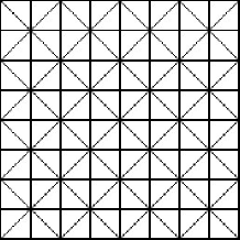
. The meshes we use are uniform ones composed of squares, each of
them being cut into 8 triangles as displayed on Figure
1 for . The refinement strategy is an
uniform one so that the value of the mesh size between two
consecutive meshes is twice smaller.
Figure 1: Mesh level corresponding to and .
In order to validate the reliability of the estimator, we
consider the ”discrete error” given by
where stands for the piecewise -discontinuous
interpolation of on the mesh . This
discrete error is defined by approximating the norm
of arising in (see (9)) by its discrete
locally computable version defined by
(30)
The computation of is now an easy
task and simply corresponds to the determination of the largest
eigenvalue of a classical generalized finite dimensional eigenvalue
problem. In order to validate the reliability of the estimator
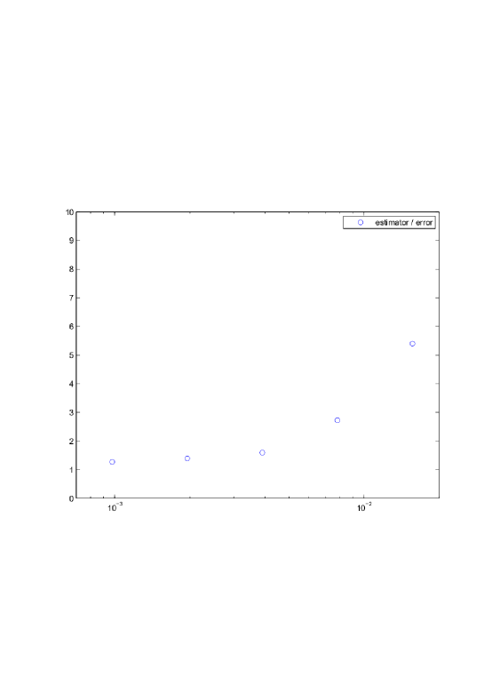
according to theorem 4.5, the error estimator is
defined by
and we plot on Figure 2 the evolution of
the computed effectivity index versus .
Here, the values of as well as are respectively
computed in the same manner as in [15] and
[30], in order to obtain relevant choices
as required by theorem 5.4 to ensure the efficiency of the estimator.
Practically, some fluxes through the edges of
each triangle of the mesh are needed, and have to be computed by
solving local linear problems. In fact, in our tests, these values
are explicitely defined. For , we use , where
denotes the averaged value on the triangles on each side of of evaluated at the middle of .
For , we use . Here, is the averaged value over the triangles surrouding the node of the piecewise constant function on each triangle
, and stands for the classical -Lagrange basis function associated with the node .
Moreoever, for the construction of , the
Argyris basis functions have to be used (see section 4 of [30] as well as [17] for the practical
implementation).
From (16) we have .
The Poincaré-Friedrichs constant is here equal to
since is the unit square. Because of the
kind of meshes used (see Figure 1), we have
and (see annex
7.2). Finally, it can be proved [23]
that on the unit square, ,
hence below we take this upper bound for (while it is
conjectured that , see [16]).
Figure 2: versus .
As expected by the theory, it can be observed that the
computed effectivity index is larger than one. Moreover, it converges
towards a constant close to one when goes towards zero, so that the proposed
estimator is asymptotically exact.
7.2 Evaluation of for the triangulation of section 6
With the definitions given above, let us consider
an affine function on , so that on . With
and defined in the proof of lemma 4.3 and the
triangular inequality, we get
[1]
M. Ainsworth and J. Oden.
A posteriori error estimation in finite element analysis.
John Wiley and Sons, 2000.
[2]
I. Babuška and T. Strouboulis.
The finite element methods and its reliability.
Clarendon Press, Oxford.
[3]
K.J. Bathe, F. Brezzi and M. Fortin. Mixed-interpolated elements for Reissner-Mindlin plates. Int. J. Num. Meths. Engrg, Volume 28, pp 1787-1801, 1989.
[4]
K.J. Bathe and E. Dvorkin. A four-node plate bending element based on Mindlin-Reissner plate theory and a mixed interpolation. Int. J. Num. Meths. Engrg., 21, pp 367-383, 1985.
[5]
L. Beirão da Veiga, C. Chinosi, C. Lovadina, and R. Stenberg.
A-priori and a-posteriori error analysis for a family of
Reissner-Mindlin plate elements.
BIT, 48(2):189–213, 2008.
[6]
D. Braess and J. Schöberl.
Equilibrated residual error estimator for edge elements.
Math. Comp., 77(262):651–672, 2008.
[7]
S. C. Brenner and L. R. Scott.
The mathematical theory of finite element methods.
Springer, New York, 1994.
[8]
F. Brezzi and M. Fortin.
Mixed and hybrid finite element methods.
Springer-Verlag, New-York, 1991.
[9]
C. Carstensen.
Residual-based a posteriori error estimate for a nonconforming
Reissner-Mindlin plate finite element.
SIAM J. Numer. Anal., 39(6):2034–2044 (electronic), 2002.
[10] C. Cartensen and S.A Funken.
Constants in Clément-interpolation error and residual based
a posteriori error estimates in Finite Element Methods. East-West
J. Numer. Math., Vol 8, No 3. pp 153-175, 2000.
[11]
C. Cartensen and Jun Hu. A posteriori error analysis for
conforming MITC elements for Reissner-Mindlin plates. Mathematics
of computation, 77, 262, pp 611-632, 2008.
[12]
C. Carstensen and J. Schöberl.
Residual-based a posteriori error estimate for a mixed Reißner-Mindlin plate finite element method.
Numer. Math., 103(2):225–250, 2006.
[13]
P. G. Ciarlet.
The finite element method for elliptic problems.
North-Holland, Amsterdam, 1978.
[14]
Ph. Clement. Approximation by finite element functions using local regularization. RAIRO R2, pp 77-84, 1975.
[15]
S. Cochez-Dhondt and S. Nicaise. A posteriori error estimators
based on equilibrated fluxes. Computational Methods in Applied
Mathematics, Vol 10, pp 49-68, 2010.
[17] V. Domínguez and F.-J. Sayas. A
simple Matlab implementation of the Argyris element. ACM
Trans. Math. Software 35, no. 2, Art. 16, 11 pp, 2009.
[18]
R. Duran, E. Hernandez, L. Hervella-Nieto, E. Liberman and R. Rodriguez. Error estimates for lower-order isoparametric quadrilateral finite elements for plates. SIAM J. Numer. Anal., 41, pp 1751-1772, 2003.
[19]
Ricardo Durán and Elsa Liberman. On mixed finite element
methods for the Reissner-Mindlin plate model. Mathematics of Computation, 58, 198, pp 561-573, 1992.
[20]
A. Ern, S. Nicaise, and M. Vohralík.
An accurate flux reconstruction for
discontinuous Galerkin approximations of elliptic problems.
C. R. Math. Acad. Sci. Paris, 345(12):709–712, 2007.
[21]
M.E. Frolov, P. Neittaanmäki and S.I. Repin. Guaranteed
functional error estimates for the Reissner-Mindlin plate problem.
Journal of Mathematical Sciences, 132, 4, pp 553-561, 2006.
[22]
V. Girault and P.-A. Raviart.
Finite elements methods for Navier-Stokes equations, Theory and
Algorithms.
Springer Series in Computational Mathematics, Berlin, 1986.
[23]
C. O. Horgan and L. E. Payne.
On inequalities of Korn, Friedrichs and Babuška-Aziz.
Arch. Rational Mech. Anal., 82(2):165–179, 1983.
[24]
J. Hu and Y. Huang.
A posteriori error analysis of finite element methods for Reissner-Mindlin plates.
SIAM J. Numer. Anal., 47 (6):4446-4472, 2010.
[25]
P. Ladevèze and D. Leguillon.
Error estimate procedure in the finite element method and
applications.
SIAM J. Numer. Anal., 20:485–509, 1983.
[26]
E. Liberman.
A posteriori error estimator for a mixed finite element method for
Reissner-Mindlin plate.
Math. Comp., 70(236):1383–1396 (electronic), 2001.
[27]
C. Lovadina and R. Stenberg.
A posteriori error analysis of the linked interpolation technique for
plate bending problems.
SIAM J. Numer. Anal., 43(5):2227–2249 (electronic), 2005.
[28]
R. Luce and B. Wohlmuth.
A local a posteriori error estimator based on equilibrated fluxes.
SIAM J. Numer. Anal., 42:1394–1414, 2004.
[29]
P. Neittaanmaäki and S. Repin.
Reliable methods for computer simulation: error control and a
posteriori error estimates., volume 33 of Studies in Mathematics and
its applications.
Elsevier, Amsterdam, 2004.
[30]
S. Nicaise, K. Witowski, and B. I. Wohlmuth.
An a posteriori error estimator for the Lamé equation based on
equilibrated fluxes.
IMA J. Numer. Anal., 28(2):331–353, 2008.
[31]
R. Stenberg and M. Suri. An hp error analysis of MITC plate elements. SIAM J. Numer. Anal. 34, pp 544-568, 1997.
[32]
R. Verfurth.
A review of a posteriori error estimation and adaptive
mesh-refinement techniques.
Teubner Skripten zur Numerik, 1996.