Probabilistic Inferences in Bayesian Networks

Abstract

Bayesian network is a complete model for the variables and their relationships, it can be used to answer probabilistic queries about them. A Bayesian network can thus be considered a mechanism for automatically applying Bayes’ theorem to complex problems. In the application of Bayesian networks, most of the work is related to probabilistic inferences. Any variable updating in any node of Bayesian networks might result in the evidence propagation across the Bayesian networks. This paper sums up various inference techniques in Bayesian networks and provide guidance for the algorithm calculation in probabilistic inference in Bayesian networks.

1 Introduction

Because a Bayesian network is a complete model for the variables and their relationships, it can be used to answer probabilistic queries about them. For example, the network can be used to find out updated knowledge of the state of a subset of variables when other variables (the evidence variables) are observed. This process of computing the posterior distribution of variables given evidence is called probabilistic inference. A Bayesian network can thus be considered a mechanism for automatically applying Bayes’ theorem to complex problems.

In the application of Bayesian networks, most of the work is related to probabilistic inferences. Any variable updating in any node of Bayesian networks might result in the evidence propagation across the Bayesian networks. How to examine and execute various inferences is the important task in the application of Bayesian networks.

This chapter will sum up various inference techniques in Bayesian networks and provide guidance for the algorithm calculation in probabilistic inference in Bayesian networks. Information systems are of discrete event characteristics, this chapter mainly concerns the inferences in discrete events of Bayesian networks.

2 The Semantics of Bayesian Networks

The key feature of Bayesian networks is the fact that they provide a method for decomposing a probability distribution into a set of local distributions. The independence semantics associated with the network topology specifies how to combine these local distributions to obtain the complete joint probability distribution over all the random variables represented by the nodes in the network. This has three important consequences.

Firstly, naively specifying a joint probability distribution with a table requires a number of values exponential in the number of variables. For systems in which interactions among the random variables are sparse, Bayesian networks drastically reduce the number of required values.

Secondly, efficient inference algorithms are formed in that work by transmitting information between the local distributions rather than working with the full joint distribution.

Thirdly, the separation of the qualitative representation of the influences between variables from the numeric quantification of the strength of the influences has a significant advantage for knowledge engineering. When building a Bayesian network model, one can focus first on specifying the qualitative structure of the domain and then on quantifying the influences. When the model is built, one is guaranteed to have a complete specification of the joint probability distribution.

The most common computation performed on Bayesian networks is the determination of the posterior probability of some random variables, given the values of other variables in the network. Because of the symmetric nature of conditional probability, this computation can be used to perform both diagnosis and prediction. Other common computations are: the computation of the probability of the conjunction of a set of random variables, the computation of the most likely combination of values of the random variables in the network and the computation of the piece of evidence that has or will have the most influence on a given hypothesis.

A detailed discussion of inference techniques in Bayesian networks can be found in the book by Pearl [Pearl, 2000].

• Probabilistic semantics. Any complete probabilistic model of a domain must, either explicitly or implicitly, represent the joint distribution which the probability of every possible event as defined by the values of all the variables. There are exponentially many such events, yet Bayesian networks achieve compactness by factoring the joint distribution into local, conditional distributions for each variable given its parents. If $x_{i}$ denotes some value of the variable $X_{i}$ and $\pi(x_{i})$ denotes some set of values for $X_{i}$’s parents $\pi(x_{i})$, then $P(x_{i}|\pi(x_{i}))$ denotes this conditional distribution. For example, $P(x_{4}|x_{2},x_{3})$ is the probability of wetness given the values of sprinkler and rain. Here $P(x_{4}|x_{2},x_{3})$ is the brief of $P(x_{4}|\{x_{2},x_{3}\})$. The set parentheses are omitted for the sake of readability. We use the same expression in this thesis. The global semantics of Bayesian networks specifies that the full joint distribution is given by the product

  $$P(x_{1},\ldots,x_{n})=\prod_{i}P(x_{i}|\pi(x_{i}))$$ (1)

  Equation 1 is also called the chain rule for Bayesian networks.

  

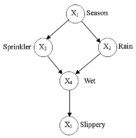
  Figure 1: Causal Influences in A Bayesian Network.

  In the example Bayesian network in Figure 1, we have

  $$P(x_{1},x_{2},x_{3},x_{4},x_{5})=P(x_{1})P(x_{2}|x_{1})P(x_{3}|x_{1})P(x_{4}|x_{2},x_{3})P(x_{5}|x_{4})$$ (2)

  Provided the number of parents of each node is bounded, it is easy to see that the number of parameters required grows only linearly with the size of the network, whereas the joint distribution itself grows exponentially. Further savings can be achieved using compact parametric representations, such as noisy-OR models, decision tress, or neural networks, for the conditional distributions [Pearl, 2000].

  There are also entirely equivalent local semantics, which assert that each variable is independent of its non-descendants in the network given its parents. For example, the parents of $X_{4}$ in Figure 1 are $X_{2}$ and $X_{3}$ and they render $X_{4}$ independent of the remaining non-descendant, $X_{1}$. That is,

  $$P(x_{4}|x_{1},x_{2},x_{3})=P(x_{4}|x_{2},x_{3})$$ (3)

  The collection of independence assertions formed in this way suffices to derive the global assertion in Equation 2, and vice versa. The local semantics are most useful in constructing Bayesian networks, because selecting as parents the direct causes of a given variable automatically satisfies the local conditional independence conditions. The global semantics lead directly to a variety of algorithms for reasoning.

• Evidential reasoning. From the product specification in Equation 2, one can express the probability of any desired proposition in terms of the conditional probabilities specified in the network. For example, the probability that the sprinkler was on, given that the pavement is slippery, is

  $$P(X_{3}=on|X_{5}=true)$$ (4)

  $$=\frac{P(X_{3}=on,X_{5}=true)}{P(X_{5}=true)}$$

  $$=\frac{\sum_{x_{1},x_{2},x_{4}}P(x_{1},x_{2},X_{3}=on,x_{4},X_{5}=true)}{\sum_{x_{1},x_{2},x_{3},x_{4}}P(x_{1},x_{2},x_{3},x_{4},X_{5}=true)}$$

  $$=\frac{\sum_{x_{1},x_{2},x_{4}}P(x_{1})P(x_{2}|x_{1})P(X_{3}=on|x_{1})P(x_{4}|x_{2},X_{3}=on)P(X_{5}=true|x_{4})}{\sum_{x_{1},x_{2},x_{3},x_{4}}P(x_{1})P(x_{2}|x_{1})P(x_{3}|x_{1})P(x_{4}|x_{2},x_{3})P(X_{5}=true|x_{4})}$$

  These expressions can often be simplified in the ways that reflect the structure of the network itself.

  It is easy to show that reasoning in Bayesian networks subsumes the satisfiability problem in propositional logic and hence reasoning is NP-hard [Cooper, 1990]. Monte Carlo simulation methods can be used for approximate inference [Pearl, 1987], given that estimates are gradually improved as the sampling proceeds. (Unlike join-tree methods, these methods use local message propagation on the original network structure.) Alternatively, variational methods [Jordan et al., 1998] provide bounds on the true probability.

• Functional Bayesian networks. The networks discussed so far are capable of supporting reasoning about evidence and about actions. Additional refinement is necessary in order to process counterfactual information. For example, the probability that ”the pavement would not have been slippery had the sprinkler been OFF, given that the sprinkler is in fact ON and that the pavement is in fact slippery” cannot be computed from the information provided in Figure 1 and Equation 2. Such counterfactual probabilities require a specification in the form of functional networks, where each conditional probability $P(x_{i}|\pi(i))$ is replaced by a functional relationship $x_{i}=f_{i}(\pi(i),\epsilon_{i})$, where $\epsilon_{i}$ is a stochastic (unobserved) error term. When the functions $f_{i}$ and the distributions of $\epsilon_{i}$ are known, all counterfactual statements can be assigned unique probabilities, using evidence propagation in a structure called a ”twin network”. When only partial knowledge about the functional form of $f_{i}$ is available, bounds can be computed on the probabilities of counterfactual sentences [Balke & Pearl, 1995] [Pearl, 2000].

• Causal discovery. One of the most exciting prospects in recent years has been the possibility of using Bayesian networks to discover causal structures in raw statistical data [Pearl & Verma, 1991] [Spirtes et al., 1993] [Pearl, 2000], which is a task previously considered impossible without controlled experiments. Consider, for example, the following pattern of dependencies among three events: $A$ and $B$ are dependent, $B$ and $C$ are dependent, yet $A$ and $C$ are independent. If you ask a person to supply an example of three such events, the example would invariably portray $A$ and $C$ as two independent causes and $B$ as their common effect, namely, $A\rightarrow B\leftarrow C$. Fitting this dependence pattern with a scenario in which $B$ is the cause and $A$ and $C$ are the effects is mathematically feasible but very unnatural, because it must entail fine tuning of the probabilities involved; the desired dependence pattern will be destroyed as soon as the probabilities undergo a slight change.

  Such thought experiments tell us that certain patterns of dependency, which are totally void of temporal information, are conceptually characteristic of certain causal directionalities and not others. When put together systematically, such patterns can be used to infer causal structures from raw data and to guarantee that any alternative structure compatible with the data must be less stable than the one(s) inferred; namely, slight fluctuations in parameters will render that structure incompatible with the data.

• Plain beliefs. In mundane decision making, beliefs are revised not by adjusting numerical probabilities but by tentatively accepting some sentences as ”true for all practical purposes”. Such sentences, called plain beliefs, exhibit both logical and probabilistic characters. As in classical logic, they are propositional and deductively closed; as in probability, they are subject to retraction and to varying degrees of entrenchment. Bayesian networks can be adopted to model the dynamics of plain beliefs by replacing ordinary probabilities with non-standard probabilities, that is, probabilities that are infinitesimally close to either zero or one [Goldszmidt & Pearl, 1996].

• Models of cognition. Bayesian networks may be viewed as normative cognitive models of propositional reasoning under uncertainty [Pearl, 2000]. They handle noise and partial information by using local, distributed algorithm for inference and learning. Unlike feed forward neural networks, they facilitate local representations in which nodes correspond to propositions of interest. Recent experiments [Tenenbaum & Griffiths, 2001] suggest that they capture accurately the causal inferences made by both children and adults. Moreover, they capture patterns of reasoning that are not easily handled by any competing computational model. They appear to have many of the advantages of both the “symbolic” and the “subsymbolic” approaches to cognitive modelling.

  Two major questions arise when we postulate Bayesian networks as potential models of actual human cognition.

  Firstly, does an architecture resembling that of Bayesian networks exist anywhere in the human brain? No specific work had been done to design neural plausible models that implement the required functionality, although no obvious obstacles exist.

  Secondly, how could Bayesian networks, which are purely propositional in their expressive power, handle the kinds of reasoning about individuals, relations, properties, and universals that pervades human thought? One plausible answer is that Bayesian networks containing propositions relevant to the current context are constantly being assembled as needed to form a more permanent store of knowledge. For example, the network in Figure 1 may be assembled to help explain why this particular pavement is slippery right now, and to decide whether this can be prevented. The background store of knowledge includes general models of pavements, sprinklers, slipping, rain, and so on; these must be accessed and supplied with instance data to construct the specific Bayesian network structure. The store of background knowledge must utilize some representation that combines the expressive power of first-order logical languages (such as semantic networks) with the ability to handle uncertain information.

3 Reasoning Structures in Bayesian Networks

3.1 Basic reasoning structures

3.1.1 d-Separation in Bayesian Networks

d-Separation is one important property of Bayesian networks for inference. Before we define d-separation, we first look at the way that evidence is transmitted in Bayesian Networks. There are two types of evidence:

• Hard Evidence (instantiation) for a node $A$ is evidence that the state of $A$ is definitely a particular value.

• Soft Evidence for a node $A$ is any evidence that enables us to update the prior probability values for the states of $A$.

d-Separation (Definition):

Two distinct variables $X$ and $Z$ in a causal network are d-separated if, for all paths between $X$ and $Z$, there is an intermediate variable $V$ (distinct from $X$ and $Z$) such that either

• the connection is serial or diverging and $V$ is instantiated or

• the connection is converging, and neither $V$ nor any of $V$’s descendants have received evidence.

If $X$ and $Z$ are not d-separated, we call them d-connected.

3.1.2 Basic structures of Bayesian Networks

Based on the definition of d-seperation, three basic structures in Bayesian networks are as follows:

1. Serial connections

   Consider the situation in Figure 2. $X$ has an influence on $Y$, which in turn has an influence on $Z$. Obviously, evidence on $Z$ will influence the certainty of $Y$, which then influences the certainty of $Z$. Similarly, evidence on $Z$ will influence the certainty on $X$ through $Y$. On the other hand, if the state of $Y$ is known, then the channel is blocked, and $X$ and $Z$ become independent. We say that $X$ and $Z$ are d-separated given $Y$, and when the state of a variable is known, we say that it is instantiated (hard evidence).

   We conclude that evidence may be transmitted through a serial connection unless the state of the variable in the connection is known.

   

   Figure 2: Serial Connection. When $Y$ is Instantiated, it blocks the communication between $X$ and $Z$.

2. Diverging connections

   The situation in Figure 3 is called a diverging connection. Influence can pass between all the children of $X$ unless the state of $X$ is known. We say that $Y_{1},Y_{2},\ldots,Y_{n}$ are d-separated given $X$.

   Evidence may be transmitted through a diverging connection unless it is instantiated.

   

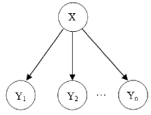
   Figure 3: Diverging Connection. If $X$ is instantiated, it blocks the communication between its children.

3. Converging connections

   

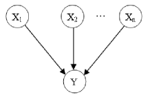
   Figure 4: Converging Connection. If $Y$ changes certainty, it opens for the communication between its parents.

   A description of the situation in Figure 4 requires a little more care. If nothing is known about $Y$ except what may be inferred from knowledge of its parents $X_{1},\ldots,X_{n}$, then the parents are independent: evidence on one of the possible causes of an event does not tell us anything about other possible causes. However, if anything is known about the consequences, then information on one possible cause may tell us something about the other causes.

   This is the explaining away effect illustrated in Figure 1. $X_{4}$ (pavement is wet) has occurred, and $X_{3}$ (the sprinkler is on) as well as $X_{2}$ (it’s raining) may cause $X_{4}$. If we then get the information that $X_{2}$ has occurred, the certainty of $X_{3}$ will decrease. Likewise, if we get the information that $X_{2}$ has not occurred, then the certainty of $X_{3}$ will increase.

The three preceding cases cover all ways in which evidence may be transmitted through a variable.

4 Classification of Inferences in Bayesian Networks

In Bayesian networks, 4 popular inferences are identified as:

1. Forward Inference

   Forward inferences is also called predictive inference (from causes to effects). The inference reasons from new information about causes to new beliefs about effects, following the directions of the network arcs. For example, in Figure 2, $X\rightarrow Y\rightarrow Z$ is a forward inference.

2. Backward Inference

   Backward inferences is also called diagnostic inference (from effects to causes). The inference reasons from symptoms to cause, Note that this reasoning occurs in the opposite direction to the network arcs. In Figure 2 , $Z\rightarrow Y$ is a backward inference. In Figure 3 , $Y_{i}\rightarrow X(i\in[1,n])$ is a backward inference.

3. Intercausal Inference

   Intercausal inferences is also called explaining away (between parallel variables). The inference reasons about the mutual causes (effects) of a common effect (cause). For example, in Figure 4, if the $Y$ is instantiated, $X_{i}$ and $X_{j}(i,j\in[1,n])$ are dependent. The reasoning $X_{i}\leftrightarrow X_{j}(i,j\in[1,n])$ is an intercausal inference. In Figure 3, if $X$ is not instantiated, $Y_{i}$ and $Y_{j}(i,j\in[1,n])$ are dependent. The reasoning $Y_{i}\leftrightarrow Y_{j}(i,j\in[1,n])$ is an intercausal inference.

4. Mixed inference

   Mixed inferences is also called combined inference. In complex Bayesian networks, the reasoning does not fit neatly into one of the types described above. Some inferences are a combination of several types of reasoning.

4.1 Inference in Bayesian Networks

4.1.1 inference in basic models

• in Serial Connections

  • the forward inference executes with the evidence forward propagation. For example, in Figure 5, consider the inference $X\rightarrow Y\rightarrow Z$.

    

    Figure 5: Inference in Serial Connection

    If Y is instantiated, X and Z are independent, then we have following example:

    $P(Z|XY)=P(Z|Y)$;

    $P(Z^{+}|Y^{+})=0.95$;

    $P(Z^{-}|Y^{+})=0.05$;

    $P(Z^{+}|Y^{-})=0.01$;

    $P(Z^{-}|Y^{-})=0.99$;

    if Y is not instantiated, X and Z are dependent, then

    $P(Z^{+}|X^{+}Y)=P(Z^{+}|Y^{+})P(Y^{+}|X^{+})+P(Z^{+}|Y^{-})P(Y^{-}|X^{+})$

    $=0.95*0.85+0.01*0.15=0.8075+0.0015=0.809$;

    $P(Z^{-}|X^{-}Y)=P(Z^{-}|Y^{+})P(Y^{+}|X^{-})+P(Z^{-}|Y^{-})P(Y^{-}|X^{-})$

    $=0.05*0.03+0.99*0.97=0.0015+0.9603=0.9618$.

  • the backward inference executes the evidence backward propagation. For example, in Figure 5, consider the inference $Z\rightarrow Y\rightarrow X$.

    1. If $Y$ is instantiated ($P(Y^{+})=1$ or $P(Y^{-})=1)$, $X$ and $Z$ are independent, then

       $$P(X|YZ)=P(X|Y)=\frac{P(X)P(Y|X)}{P(Y)}$$ (5)

       $P(X^{+}|Y^{+}Z)=P(X^{+}|Y^{+})=\frac{P(X^{+})P(Y^{+}|X^{+})}{P(Y^{+})}=\frac{09*0.85}{1}=0.765$;

       $P(X^{+}|Y^{-}Z)=P(X^{+}|Y^{-})=\frac{P(X^{+})P(Y^{-}|X^{+})}{P(Y^{-})}=\frac{09*0.15}{1}=0.135$.

    2. If $Y$ is not instantiated, $X$ and $Z$ are dependent (See the dashed lines in Figure 5). Suppose $P(Z^{+})=1$ then

       $P(X^{+}|YZ^{+})=\frac{P(X^{+}YZ^{+})}{P(YZ^{+})}=\frac{P(X^{+}YZ^{+})}{\sum_{X}P(XYZ^{+})}$;
       

       $P(X^{+}YZ^{+})=P(X^{+}Y^{+}Z^{+})+P(X^{+}Y^{-}Z^{+})=0.9*0.85*0.95+0.9*0.15*0.05=0.72675+0.00675=0.7335$;
       

       $\sum_{X}P(XYZ^{+})=P(X^{+}Y^{+}Z^{+})+P(X^{+}Y^{-}Z^{+})+P(X^{-}Y^{+}Z^{+})+P(X^{-}Y^{-}Z^{+})\\ =0.9*0.85*0.95+0.9*0.15*0.99+0.1*0.03*0.95+0.1*0.97*0.01\\ =0.72675+0.13365+0.00285+0.00097=0.86422$;
       

       $P(X^{+}|YZ^{+})=\frac{P(X^{+}YZ^{+})}{\sum_{X}P(XYZ^{+})}=\frac{0.7335}{0.86422}=0.8487.$

  In serial connections, there is no intercausal inference.

• in Diverging Connections

  • the forward inference executes with the evidence forward propagation. For example, in Figure 6, consider the inference $Y\rightarrow X$ and $Y\rightarrow Z$, the goals are easy to obtain by nature.

    

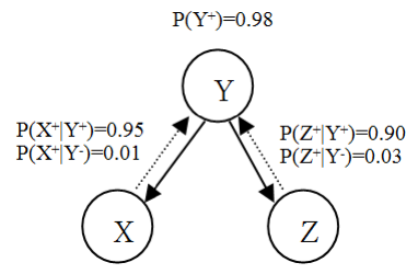
    Figure 6: Inference in Diverging Connection

  • the backward inference executes with the evidence backward propagation, see the dashed line in Figure 6, consider the inference $(XZ)\rightarrow Y$, $X$ and $Z$ are instantiated by assumption, suppose $P(X^{+}=1)$, $P(Z^{+}=1)$. Then,

    $$P(Y^{+}|X^{+}Z^{+})=\frac{P(Y^{+}X^{+}Z^{+})}{P(X^{+}Z^{+})}=\frac{P(Y^{+})P(X^{+}|Y^{+})P(Z^{+}|Y^{+})}{P(X^{+}Z^{+})}$$

    $$=\frac{0.98*0.95*0.90}{1}=0.8379$$ (6)

  • the intercausal inference executes between effects with a common cause. In Figure 6, if $Y$ is not instantiated, there exists intercausal inference in diverging connections. Consider the inference $X\rightarrow Z$,

    $P(X^{+}|YZ^{+})=\frac{P(X^{+}YZ^{+})}{P(YZ^{+})}=\frac{P(X^{+}Y^{+}Z^{+})+P(X^{+}Y^{-}Z^{+})}{P(Y^{+}Z^{+})+P(Y^{-}Z^{+})}$;

    $=\frac{0.98*0.95*0.90+0.02*0.01*0.03}{0.98*0.90+0.02*0.03}=0.94936$.

• in Converging Connections,

  • the forward inference executes with the evidence forward propagation. For example, in Figure 7, consider the inference $(XZ)\rightarrow Y$, $P(Y|XZ)$ is easy to obtain by the definition of Bayesian Network in by nature.

    

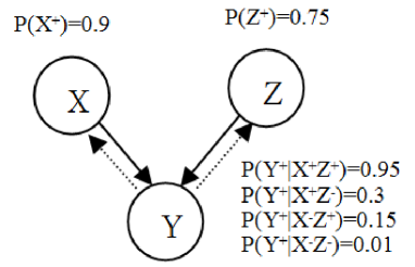
    Figure 7: Inference in Converging Connection

  • the backward inference executes with the evidence backward propagation. For example, in Figure 7, consider the inference $Y\rightarrow(XZ)$.

    $P(Y)=\sum_{XZ}P(XYZ)=\sum_{XZ}(P(Y|XZ)P(XZ))$,
    

    $P(XZ|Y)=\frac{P(Y|XZ)P(XZ)}{P(Y)}=\frac{P(Y|XZ)P(X)P(Z)}{\sum_{XZ}(P(Y|XZ)P(XZ))}$.
    

    Finally,

    $P(X|Y)=\sum_{Z}P(XZ|Y)$,

    $P(Z|Y)=\sum_{X}P(XZ|Y)$.

  • the intercausal inference executes between causes with a common effect, and the intermediate node is instantiated, then $P(Y^{+})=1$ or $P(Y^{-})=1$. In Figure 7, consider the inference $X\rightarrow Z$, suppose $P(Y^{+})=1$,

    $P(Z^{+}|X^{+}Y^{+})=\frac{P(Z^{+}X^{+}Y^{+})}{P(X^{+}Y^{+})}=\frac{P(Z^{+}X^{+}Y^{+})}{\sum_{Z}P(X^{+}Y^{+}Z)}$;
    

    $P(Z^{+}X^{+}Y^{+})=P(X^{+})P(Z^{+})P(Y^{+}|X^{+}Z^{+})$;
    

    $\sum_{Z}P(X^{+}YZ)=P(X^{+}Y^{+}Z^{+})+P(X^{+}Y^{+}Z^{-})$;
    

    $P(Z^{+}|X^{+}Y^{+})=\frac{P(Z^{+}X^{+}Y^{+})}{\sum_{Z}P(X^{+}Y^{+}Z)}=\frac{P(X^{+})P(Z^{+})P(Y^{+}|X^{+}Z^{+})}{P(X^{+}Y^{+}Z^{+})+P(X^{+}Y^{+}Z^{-})}.$

4.1.2 inference in complex model

For complex models in Bayesian networks, there are single-connected networks, multiple-connected, or event looped networks. It is possible to use some methods, such as Triangulated Graphs, Clustering and Join Trees [Bertele & Brioschi, 1972] [Finn & Thomas, 2007] [Golumbic, 1980], etc., to simplify them into a polytree. Once a polytree is obtained, the inference can be executed by the following approaches.

Polytrees have at most one path between any pair of nodes; hence they are also referred to as singly-connected networks.

Suppose $X$ is the query node, and there is some set of evident nodes $E,X\notin E$. The posterior probability (belief) is denoted as $\mathbb{B}(X)=P(X|E)$, see Figure 8.

Figure 8: Evidence Propagation in Polytree

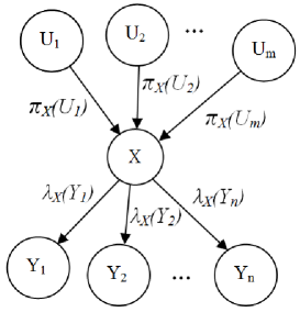
$E$ can be splitted into 2 parts: $E^{+}$ and $E^{-}$. $E^{-}$ is the part consisting of assignments to variables in the subtree rooted at $X$, $E^{+}$ is the rest of it.

$\pi_{X}(E^{+})=P(X|E^{+})$

$\lambda_{X}(E^{-})=P(E^{-}|X)$

$$\mathbb{B}(X)=P(X|E)=P(X|E^{+}E^{-})=\frac{P(E^{-}|XE^{+})P(X|E^{+})}{P(E^{-}|E^{+})}=\frac{P(E^{-}|X)P(X|E^{+})}{P(E^{-}|E^{+})}=\alpha\pi_{X}(E^{+})\lambda_{X}(E^{-})$$ (7)

$\alpha$ is a constant independent of $X$.

where

$$\lambda_{X}(E^{-})=\{\begin{array}[]{cc}1&if\ evidence\ is\ X=x_{i}\\ 0&if\ evidence\ is\ for\ another\ x_{j}\\ \end{array}$$ (8)

$$\pi_{X}(E^{+})=\sum_{u_{1},...,u_{m}}P(X|u_{1},...,u_{m})\prod_{i}\pi_{X}(u_{i})$$ (9)

1. Forward inference in Polytree

   Node $X$ sends $\pi$ messages to its children.

   $$\pi_{X}(U)=\{\begin{array}[]{cc}1&if\ x_{i}\in X\ is\ entered\\ 0&if\ evidentce\ is\ for\ another\ value\ x_{j}\\ \sum_{u_{1},...u_{m}}P(X|u_{1},...u_{m})\prod_{i}\pi_{X}(u_{i})&otherwise\end{array}$$ (10)

2. Backward inference in Polytree Node $X$ sends new $\lambda$ messages to its parents.

   $$\lambda_{X}(Y)=\prod_{y_{j}\in Y}[\sum_{j}P(y_{j}|X)\lambda_{X}(y_{j})]$$ (11)

4.2 Related Algorithms for Probabilistic Inference

Various types of inference algorithms exist for Bayesian networks [Lauritzen & Spiegelhalter, 1988] [Pearl, 1988] [Pearl, 2000] [Neal, 1993]. Each class offers different properties and works better on different classes of problems, but it is very unlikely that a single algorithm can solve all possible problem instances effectively. Every resolution is always based on a particular requirement. It is true that almost all computational problems and probabilistic inference using general Bayesian networks have been shown to be NP-hard by Cooper [Cooper, 1990].

In the early 1980’s, Pearl published an efficient message propagation inference algorithm for polytrees [Kim & Pearl, 1983] [Peal, 1986]. The algorithm is exact, and has polynomial complexity in the number of nodes, but works only for singly connected networks. Pearl also presented an exact inference algorithm for multiple connected networks called loop cutset conditioning algorithm [Peal, 1986]. The loop cutset conditioning algorithm changes the connectivity of a network and renders it singly connected by instantiating a selected subset of nodes referred to as a loop cutset. The resulting single connected network is solved by the polytree algorithm, and then the results of each instantiation are weighted by their prior probabilities. The complexity of this algorithm results from the number of different instantiations that must be considered. This implies that the complexity grows exponentially with the size of the loop cutest being $O(d^{c})$, where $d$ is the number of values that the random variables can take, and $c$ is the size of the loop cutset. It is thus important to minimize the size of the loop cutset for a multiple connected network. Unfortunately, the loop cutset minimization problem is NP-hard. A straightforward application of Pearl’s algorithm to an acyclic digraph comprising one or more loops invariably leads to insuperable problems [Koch & Westphall, 2001] [Neal, 1993].

Another popular exact Bayesian network inference algorithm is Lauritzen and Spiegelhalter’s clique-tree propagation algorithm [Lauritzen & Spiegelhalter, 1988]. It is also called a ”clustering” algorithm. It first transforms a multiple connected network into a clique tree by clustering the triangulated moral graph of the underlying undirected graph and then performs message propagation over the clique tree. The clique propagation algorithm works efficiently for sparse networks, but still can be extremely slow for dense networks. Its complexity is exponential in the size of the largest clique of the transformed undirected graph.

In general, the existent exact Bayesian network inference algorithms share the property of run time exponentiality in the size of the largest clique of the triangulated moral graph, which is also called the induced width of the graph [Lauritzen & Spiegelhalter, 1988].

5 Conclusion

This chapter summarizes the popular inferences methods in Bayesian networks. The results demonstrates that the evidence can propagated across the Bayesian networks by any links, whatever it is forward or backward or intercausal style. The belief updating of Bayesian networks can be obtained by various available inference techniques. Theoretically, exact inferences in Bayesian networks is feasible and manageable. However, the computing and inference is NP-hard. That means, in applications, in complex huge Bayesian networks, the computing and inferences should be dealt with strategically and make them tractable. Simplifying the Bayesian networks in structures, pruning unrelated nodes, merging computing, and approximate approaches might be helpful in the inferences of large scale Bayeisan networks.

References

- [Balke & Pearl, 1995] A. Balke and J. Pearl. Counterfactuals and policy analysis in structural models. Proceedings of the Eleventh Conference on Uncertainty in Artificial Intelligence, pages 11-18, 1995. Morgan Kaufmann.
- [Bertele & Brioschi, 1972] Bertele, U. and Brioschi, F. (1972). Nonserial Dynamic Programming. Academic Press, London, ISBN-13: 978-0120934508.
- [Cooper, 1990] G. Cooper. Computational complexity of probabilistic inference using Bayesian belief networks. Artificial Intelligence, 42:393-405, 1990.
- [Finn & Thomas, 2007 ] Finn V. Jensen and Thomas D. Nielsen (2007). Bayesian Networks and Decision Graphs. Springer, ISBN-13:978-0-387-68281-5.
- [Golumbic, 1980] Golumbic, M. C. (1980). Algorithmic Graph Theory and Perfect Graphs. Academic Press, London,ISBN-13: 978-0122892608.
- [Goldszmidt & Pearl, 1996] M. Goldszmidt and J. Pearl. Qualitative Probabilities for Default Reasoning, Belief Revision, and Causal Modeling. Artificial Intelligence, 84(1-2): 57-112, July 1996.
- [Jordan et al., 1998] M. I. Jordan, Z. Ghahramani, T. S. Jaakkola and L. K. Saul. An Introduction to Variational Methods for Graphical Models. M. I. Jordan (Ed.), Learning in Graphical Models. Kluwer, Dordrecht, The Netherlands, 1998.
- [Kim & Pearl, 1983] Jin H. Kim and Judea Pearl. A computational model for combined causal and diagnostic reasoning in inference systems. In Proceedings of the Eighth International Joint Conference on Artificial Intelligence (IJCAI-83), pages 190-193, 1983. Morgan Kaufmann.
- [ Koch & Westphall, 2001] F. L. Koch, and C. B. Westphall. Decentralized Network Management Using Distributed Artificial Intelligence. Journal of Network and systems management, Vol. 9, No. 4, December 2001.
- [Lauritzen & Spiegelhalter, 1988] S. L. Lauritzen and D. J. Spiegelhalter. Local Computations with Probabilities on Graphical Structures and Their Application to Expert Systems. Journal of the Royal Statistical Society, Series B 50:157-224, 1988.
- [Neal, 1993] R. M. Neal, Probabilistic Inference Using Markov Chain Monte Carlo methods, Tech. Rep. CRG-TR93-1, University of Toronto, Department of Computer Science, 1993.
- [Peal, 1986] J. Pearl. A constraint-propagation approach to probabilistic reasoning, Uncertainty in Artificial Intelligence. North-Holland, Amsterdam, pages 357-369, 1986.
- [Pearl, 1987] J. Pearl. Evidential Reasoning Using Stochastic Simulation of Causal Models. Artificial Intelligence, 32:247-257, 1987.
- [Pearl, 1988] J. Pearl. Probabilistic Reasoning in Intelligent Systems: Networks of Plausible Inference. Morgan Kaufmann, San Mateo, CA, 1988.
- [Pearl, 2000] J. Pearl. Causality: Models, Reasoning, and Inference. Cambridge, England: Cambridge University Press. New York, NY, 2000.
- [Pearl & Verma, 1991] J. Pearl and T. Verma. A theory of inferred causation. J. A. Allen, R. Fikes and E. Sandewall (Eds.), Principles of Knowledge Representation and Reasoning. Proceedings of the Second International Conference, pages 441-452. Morgan Kaufmann, San Mateo, CA, 1991.
- [Spirtes et al., 1993] P. Spirtes, C. Glymour and R. Scheines. Causation, Prediction, and Search. Springer-Verlag, New York, 1993.
- [Tenenbaum & Griffiths, 2001] J. B. Tenenbaum and T. L. Griffiths. Structure learning in human causal induction. Advances in Neural Information Processing Systems, volume 13, Denver, Colorado, 2001. MIT Press.