Pore-Scale Modeling of Non-Newtonian
Flow in Porous Media
Taha Sochi
A dissertation submitted to the
Department of Earth Science and Engineering
Imperial College London
in fulfillment of the requirements for the degree of
Doctor of Philosophy

Abstract
The thesis investigates the flow of non-Newtonian fluids in porous media using network modeling. Non-Newtonian fluids occur in diverse natural and synthetic forms and have many important applications including in the oil industry. They show very complex time and strain dependent behavior and may have initial yield stress. Their common feature is that they do not obey the simple Newtonian relation of proportionality between stress and rate of deformation. They are generally classified into three main categories: time-independent in which strain rate solely depends on the instantaneous stress, time-dependent in which strain rate is a function of both magnitude and duration of the applied stress and viscoelastic which shows partial elastic recovery on removal of the deforming stress and usually demonstrates both time and strain dependency.

The methodology followed in this investigation is pore-scale network modeling. Two three-dimensional topologically-disordered networks representing a sand pack and Berea sandstone were used. The networks are built from topologically-equivalent three-dimensional voxel images of the pore space with the pore sizes, shapes and connectivity reflecting the real medium. Pores and throats are modeled as having triangular, square or circular cross-section by assigning a shape factor, which is the ratio of the area to the perimeter squared and is obtained from the pore space description. An iterative numerical technique is used to solve the pressure field and obtain the total volumetric flow rate and apparent viscosity. In some cases, analytical expressions for the volumetric flow rate in a single tube are derived and implemented in each throat to simulate the flow in the pore space.

The time-independent category of the non-Newtonian fluids is investigated using two time-independent fluid models: Ellis and Herschel-Bulkley. Thorough comparison between the two random networks and the uniform bundle-of-tubes model is presented. The analysis confirmed the reliability of the non-Newtonian network model used in this study. Good results are obtained, especially for the Ellis model, when comparing the network model results to experimental data sets found in the literature. The yield-stress phenomenon is also investigated and several numerical algorithms were developed and implemented to predict threshold yield pressure of the network.

An extensive literature survey and investigation were carried out to understand the phenomenon of viscoelasticity and clearly identify its characteristic features, with special attention paid to flow in porous media. The extensional flow and viscosity and converging-diverging geometry were thoroughly examined as the basis of the peculiar viscoelastic behavior in porous media. The modified Bautista-Manero model, which successfully describes shear-thinning, elasticity and thixotropic time-dependency, was identified as a promising candidate for modeling the flow of viscoelastic materials which also show thixotropic attributes. An algorithm that employs this model to simulate steady-state time-dependent viscoelastic flow was implemented in the non-Newtonian code and the initial results were analyzed. The findings are encouraging for further future development.

The time-dependent category of the non-Newtonian fluids was examined and several problems in modeling and simulating the flow of these fluids were identified. Several suggestions were presented to overcome these difficulties.

Acknowledgements
I would like to thank

• My supervisor Prof. Martin Blunt for his guidance and advice and for offering this opportunity to study non-Newtonian flow in porous media at Imperial College London funded by the Pore-Scale Modeling Consortium.

• Our sponsors in the Pore-Scale Modeling Consortium (BHP, DTI, ENI, JOGMEC, Saudi Aramco, Schlumberger, Shell, Statoil and Total), for their financial support, with special thanks to Schlumberger for funding this research.

• Schlumberger Cambridge Research Centre for hosting a number of productive meetings in which many important aspects of the work presented in this thesis were discussed and assessed.

• Dr Valerie Anderson and Dr John Crawshaw for their help and advice with regards to the Tardy algorithm.

• The Internal Examiner Prof. Geoffrey Maitland from the Department of Chemical Engineering Imperial College London, and the External Examiner Prof. William Rossen from the Faculty of Civil Engineering and Geosciences Delft University for their helpful remarks and corrections which improved the quality of this work.

• Staff and students in Imperial College London for their kindness and support.

• Family and friends for support and encouragement, with special thanks to my wife.

Nomenclature

Symbol	Meaning and units
$\alpha$	parameter in Ellis model (—)
$\dot{\gamma}$	strain rate (s-1)
$\dot{\gamma}_{c}$	characteristic strain rate (s-1)
$\dot{\gamma}_{cr}$	critical shear rate (s-1)
$\dot{\gamma}$	rate-of-strain tensor
$\epsilon$	porosity (—)
$\varepsilon$	elongation (—)
$\dot{\varepsilon}$	elongation rate (s-1)
$\lambda$	structural relaxation time in Fredrickson model (s)
$\lambda_{1}$	relaxation time (s)
$\lambda_{2}$	retardation time (s)
$\lambda_{c}$	characteristic time of fluid (s)
$\lambda^{{}^{\prime}}$	first time constant in Godfrey model (s)
$\lambda^{{}^{\prime\prime}}$	second time constant in Godfrey model (s)
$\lambda_{s}$	time constant in Stretched Exponential Model (s)
$\mu$	viscosity (Pa.s)
$\mu_{a}$	apparent viscosity (Pa.s)
$\mu_{e}$	effective viscosity (Pa.s)
$\mu_{{}_{i}}$	initial-time viscosity (Pa.s)
$\mu_{{}_{inf}}$	infinite-time viscosity (Pa.s)
$\mu_{o}$	zero-shear viscosity (Pa.s)
$\mu_{s}$	shear viscosity (Pa.s)
$\mu_{x}$	extensional (elongational) viscosity (Pa.s)
$\mu_{\infty}$	infinite-shear viscosity (Pa.s)
$\Delta\mu^{{}^{\prime}}$	viscosity deficit associated with $\lambda^{{}^{\prime}}$ in Godfrey model (Pa.s)
$\Delta\mu^{{}^{\prime\prime}}$	viscosity deficit associated with $\lambda^{{}^{\prime\prime}}$ in Godfrey model (Pa.s)
$\rho$	fluid mass density (kg.m-3)
$\tau$	stress (Pa)
$\tau$	stress tensor
$\tau_{{}_{1/2}}$	stress when $\mu=\mu_{o}/2$ in Ellis model (Pa)
$\tau_{o}$	yield-stress (Pa)
$\tau_{w}$	stress at tube wall ($=\Delta PR/2L$) (Pa)
$\delta\tau$	small change in stress (Pa)
$\phi$	porosity (—)
$\verb| |$
a	acceleration vector
a	magnitude of acceleration (m.s-2)
$a$	exponent in truncated Weibull distribution (—)
$b$	exponent in truncated Weibull distribution (—)
$c$	dimensionless constant in Stretched Exponential Model (—)
$C$	consistency factor in Herschel-Bulkley model (Pa.sn)
$C^{{}^{\prime}}$	tortuosity factor (—)
$C^{{}^{\prime\prime}}$	packed bed parameter (—)
$De$	Deborah number (—)
$D_{p}$	particle diameter (m)
$E$	elastic modulus (Pa)
${\mbox{\bf{e}}}_{z}$	unit vector in $z$-direction
$f_{e}$	scale factor for the entry of corrugated tube (—)
$f_{m}$	scale factor for the middle of corrugated tube (—)
F	force vector
$G$	geometric conductance (m4)
$G^{\prime}$	flow conductance (m3.Pa-1.s-1)
$Go$	elastic modulus (Pa)
$k$	parameter in Fredrickson model (Pa-1)
$K$	absolute permeability (m2)
$L$	tube length (m)
$l_{c}$	characteristic length of the flow system (m)
$m$	mass (kg)
$n$	flow behavior index (—)
$\overline{n}$	average power-law behavior index inside porous medium (—)
$N_{1}$	first normal stress difference (Pa)
$N_{2}$	second normal stress difference (Pa)
$P$	pressure (Pa)
$P_{y}$	yield pressure (Pa)
$\Delta P$	pressure drop (Pa)
$\Delta P_{th}$	threshold pressure drop (Pa)
$\nabla P$	pressure gradient (Pa.m-1)
$\nabla P_{th}$	threshold pressure gradient (Pa.m-1)
$q$	Darcy velocity (m.s-1)
$Q$	volumetric flow rate (m3.s-1)
$r$	radius (m)
$R$	tube radius (m)
$Re$	Reynolds number (—)
$R_{eq}$	equivalent radius (m)
$R_{max}$	maximum radius of corrugated capillary
$R_{min}$	minimum radius of corrugated capillary
$\mathrm{d}r$	infinitesimal change in radius (m)
$\delta r$	small change in radius (m)
$t$	time (s)
$t_{c}$	characteristic time of flow system (s)
T	temperature (K, ∘C)
$Tr$	Trouton ratio (—)
$u_{z}$	flow speed in $z$-direction (m.s-1)
v	fluid velocity vector
$V$	variable in truncated Weibull distribution
$v_{c}$	characteristic speed of flow (m.s-1)
$We$	Weissenberg number (—)
$x$	random number between 0 and 1 (—)
$\verb| |$

Abbreviations and Notations:

$\verb| |$
(.)a	apparent
AMG	Algebraic Multi-Grid
ATP	Actual Threshold Pressure
(.)e	effective
(.)eq	equivalent
(.)exp	experimental
iff	if and only if
IPM	Invasion Percolation with Memory
k	kilo
(.)max	maximum
(.)min	minimum
mm	millimeter
MTP	Minimum Threshold Path
(.)net	network
No.	Number
PMP	Path of Minimum Pressure
(.)th	threshold
$x_{{}_{l}}$	network lower boundary in the non-Newtonian code
$x_{{}_{u}}$	network upper boundary in the non-Newtonian code
$\mu$m	micrometer
$\overset{\bigtriangledown}{\mbox{$\cdot$}}$	upper convected time derivative
$(\cdot)^{T}$	matrix transpose
vs.	versus
$|\verb| ||$	modulus
$\verb| |$

Note: units, when relevant, are given in the SI system. Vectors and tensors are marked with boldface. Some symbols may rely on the context for unambiguous identification.

Chapter 1 Introduction

Newtonian fluids are defined to be those fluids exhibiting a direct proportionality between stress $\tau$ and strain rate $\dot{\gamma}$ in laminar flow, that is

$$\tau=\mu\dot{\gamma}$$ (1.1)

where the viscosity $\mu$ is independent of the strain rate although it might be affected by other physical parameters, such as temperature and pressure, for a given fluid system. A stress versus strain rate graph will be a straight line through the origin [1, 2]. In more precise technical terms, Newtonian fluids are characterized by the assumption that the extra stress tensor, which is the part of the total stress tensor that represents the shear and extensional stresses caused by the flow excluding hydrostatic pressure, is a linear isotropic function of the components of the velocity gradient, and therefore exhibits a linear relationship between stress and the rate of strain [3, 4]. In tensor form, which takes into account both shear and extension flow components, this linear relationship is expressed by

$$\mbox{\boldmath{$\tau$}}=\mu\mbox{\boldmath{$\dot{\gamma}$}}$$ (1.2)

where $\tau$ is the extra stress tensor and $\dot{\gamma}$ is the rate-of-strain tensor which describes the rate at which neighboring particles move with respect to each other independent of superposed rigid rotations. Newtonian fluids are generally featured by having shear- and time-independent viscosity, zero normal stress differences in simple shear flow and simple proportionality between the viscosities in different types of deformation [5, 6].

All those fluids for which the proportionality between stress and strain rate is not satisfied, due to nonlinearity or initial yield-stress, are said to be non-Newtonian. Some of the most characteristic features of non-Newtonian behavior are: strain-dependent viscosity where the viscosity depends on the type and rate of deformation, time-dependent viscosity where the viscosity depends on duration of deformation, yield-stress where a certain amount of stress should be reached before the flow starts, and stress relaxation where the resistance force on stretching the fluid element will first rise sharply then decay with a characteristic relaxation time.

Non-Newtonian fluids are commonly divided into three broad groups, although in reality these classifications are often by no means distinct or sharply defined [1, 2]:

1. Time-independent fluids are those for which the strain rate at a given point is solely dependent upon the instantaneous stress at that point.

2. Viscoelastic fluids are those that show partial elastic recovery upon the removal of a deforming stress. Such materials possess properties of both fluids and elastic solids.

3. Time-dependent fluids are those for which the strain rate is a function of both the magnitude and the duration of stress and possibly of the time lapse between consecutive applications of stress. These fluids are classified as thixotropic (work softening) or rheopectic (work hardening or anti-thixotropic) depending upon whether the stress decreases or increases with time at a given strain rate and constant temperature.

Those fluids that exhibit a combination of properties from more than one of the above groups may be described as complex fluids [7], though this term may be used for non-Newtonian fluids in general.

The generic rheological behavior of the three groups of non-Newtonian fluids is graphically presented in Figures (1.1-1.5). Figure (1.1) demonstrates the six principal rheological classes of the time-independent fluids in shear flow. These represent shear-thinning, shear-thickening and shear-independent fluids each with and without yield-stress. It should be emphasized that these rheological classes are idealizations as the rheology of the actual fluids is usually more complex where the fluid may behave differently under various deformation and environmental conditions. However, these basic rheological trends can describe the actual behavior under specific conditions and the overall behavior consists of a combination of stages each modeled with one of these basic classes.

Figures (1.2-1.4) display several aspects of the rheology of the viscoelastic fluids in bulk and in situ. In Figure (1.2) a stress versus time graph reveals a distinctive feature of time-dependency largely observed in viscoelastic fluids. As seen, the overshoot observed on applying a sudden deformation cycle relaxes eventually to the equilibrium steady state. This time-dependent behavior has an impact not only on the flow development in time, but also on the dilatancy behavior observed in porous media flow under steady-state conditions where the converging-diverging geometry contributes to the observed increase in viscosity when the relaxation time characterizing the fluid becomes comparable in size to the characteristic time of the flow.

In Figure (1.3) a rheogram reveals another characteristic viscoelastic feature observed in porous media flow. The intermediate plateau may be attributed to the time-dependent nature of the viscoelastic fluid when the relaxation time of the fluid and the characteristic time of the flow become comparable in size. The converging-diverging nature of the pore structure accentuates this phenomenon where the overshoot in stress interacts with the tightening of the throats to produce this behavior. This behavior was also attributed to build-up and break-down due to sudden change in radius and hence rate of strain on passing through the converging-diverging pores [8]. This may suggest a thixotropic origin for this feature.

In Figure (1.4) a rheogram of a typical viscoelastic fluid is presented. In addition to the low-deformation Newtonian plateau and the shear-thinning region which are widely observed in many time-independent fluids and modeled by various time-independent rheological models such as Carreau and Ellis, there is a thickening region which is believed to be originating from the dominance of extension over shear at high flow rates. This behavior is mainly observed in porous media flow and the converging-diverging geometry is usually given as an explanation to the shift from shear flow to extension flow at high flow rates. However, this behavior may also be observed in bulk at high strain rates.

In Figure (1.5) the two basic classes of time-dependent fluids are presented and compared to the time-independent fluid in a graph of stress against time of deformation under constant strain rate condition. As seen, thixotropy is the equivalent in time of shear-thinning, while rheopexy is the equivalent in time of shear-thickening.

A large number of models have been proposed in the literature to model all types of non-Newtonian fluids under various flow conditions. However, it should be emphasized that most these models are basically empirical in nature and arising from curve-fitting exercises [5]. In this thesis, we investigate a few models of the time-independent, time-dependent and viscoelastic fluids.

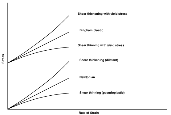
Figure 1.1: The six main classes of the time-independent fluids presented in a generic graph of stress against strain rate in shear flow.

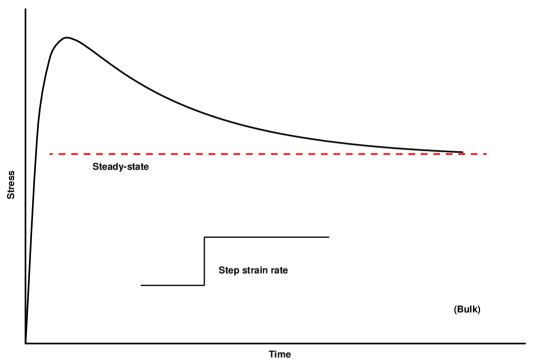
Figure 1.2: Typical time-dependence behavior of viscoelastic fluids due to delayed response and relaxation following a step increase in strain rate.

Figure 1.3: Intermediate plateau typical of in situ viscoelastic behavior due to converging-diverging geometry with the characteristic time of fluid being comparable to the time of flow.

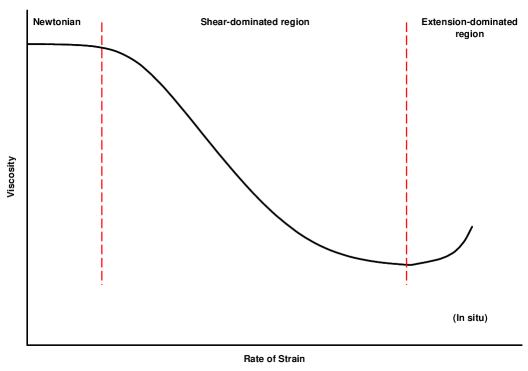
Figure 1.4: Strain hardening at high strain rates characteristic of viscoelastic fluid mainly observed in situ due to the dominance of extension over shear at high flow rates.

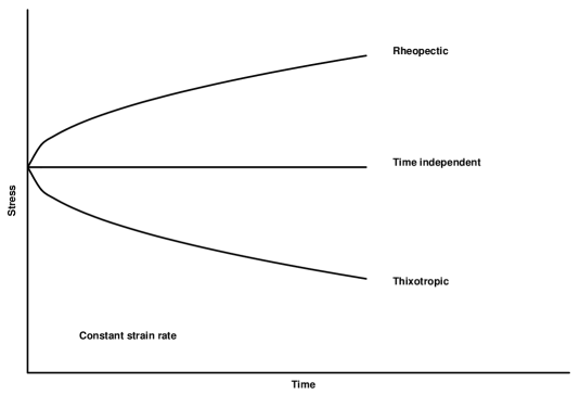
Figure 1.5: The two classes of time-dependent fluids compared to the time-independent presented in a generic graph of stress against time.

1.1 Time-Independent Fluids

Shear-rate dependence is one of the most important and defining characteristics of non-Newtonian fluids in general and time-independent fluids in particular. When a typical non-Newtonian fluid experiences a shear flow the viscosity appears to be Newtonian at low-shear rates. After this initial Newtonian plateau the viscosity is found to vary with increasing shear-rate. The fluid is described as shear-thinning or pseudoplastic if the viscosity decreases, and shear-thickening or dilatant if the viscosity increases on increasing shear-rate. After this shear-dependent regime, the viscosity reaches a limiting constant value at high shear-rate. This region is described as the upper Newtonian plateau. If the fluid sustains initial stress without flowing, it is called a yield-stress fluid.

Almost all polymer solutions that exhibit a shear-rate dependent viscosity are shear-thinning, with relatively few polymer solutions demonstrating dilatant behavior. Moreover, in most known cases of shear-thickening there is a region of shear-thinning at lower shear rates [6, 3, 5].

In this thesis, two fluid models of the time-independent group are investigated: Ellis and Herschel-Bulkley.

1.1.1 Ellis Model

This is a three-parameter model which describes time-independent shear-thinning yield-free non-Newtonian fluids. It is used as a substitute for the power-law and is appreciably better than the power-law model in matching experimental measurements. Its distinctive feature is the low-shear Newtonian plateau without a high-shear plateau. According to this model, the fluid viscosity $\mu$ is given by [9, 10, 6, 11]

$$\mu=\frac{\mu_{o}}{1+\left(\frac{\tau}{\tau_{{}_{1/2}}}\right)^{\alpha-1}}$$ (1.3)

where $\mu_{o}$ is the low-shear viscosity, $\tau$ is the shear stress, $\tau_{{}_{1/2}}$ is the shear stress at which $\mu=\mu_{o}/2$ and $\alpha$ is an indicial parameter. A generic graph demonstrating the bulk rheology, that is viscosity versus shear rate on logarithmic scale, is shown in Figure (1.6).

For Ellis fluids, the volumetric flow rate in circular cylindrical tube is given by [9, 10, 6, 11]:

$$Q=\frac{\pi R^{4}\Delta P}{8L\mu_{o}}\left[1+\frac{4}{\alpha+3}\left(\frac{R\Delta P}{2L\tau_{{}_{1/2}}}\right)^{\alpha-1}\right]$$ (1.4)

where $\mu_{o}$, $\tau_{{}_{1/2}}$ and $\alpha$ are the Ellis parameters, $R$ is the tube radius, $\Delta P$ is the pressure drop across the tube and $L$ is the tube length. The derivation of this expression is given in Appendix A.

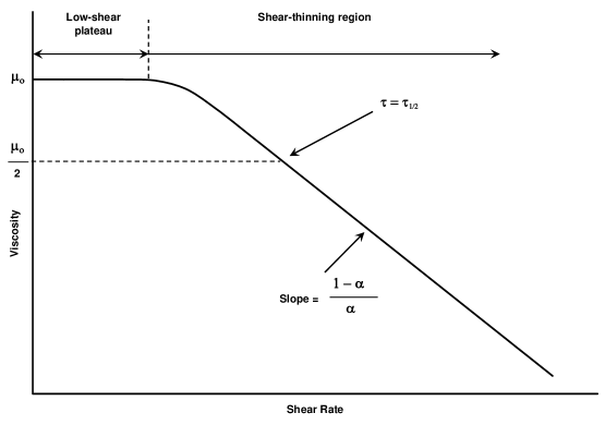
Figure 1.6: The bulk rheology of an Ellis fluid on logarithmic scale.

1.1.2 Herschel-Bulkley Model

The Herschel-Bulkley model has three parameters and can describe Newtonian and a large group of time-independent non-Newtonian fluids. It is given by [1]

$$\tau=\tau_{o}+C\dot{\gamma}^{n}\verb| |(\tau>\tau_{o})$$ (1.5)

where $\tau$ is the shear stress, $\tau_{o}$ is the yield-stress above which the substance starts flowing, $C$ is the consistency factor, $\dot{\gamma}$ is the shear rate and $n$ is the flow behavior index. The Herschel-Bulkley model reduces to the power-law, or Ostwald-de Waele model, when the yield-stress is zero, to the Bingham plastic model when the flow behavior index is unity, and to the Newton’s law for viscous fluids when both the yield-stress is zero and the flow behavior index is unity [12].

There are six main classes to this model:

1. Shear-thinning (pseudoplastic)              [$\tau_{o}=0,n<1.0$]

2. Newtonian                                            [$\tau_{o}=0,n=1.0$]

3. Shear-thickening (dilatant)                   [$\tau_{o}=0,n>1.0$]

4. Shear-thinning with yield-stress            [$\tau_{o}>0,n<1.0$]

5. Bingham plastic                                    [$\tau_{o}>0,n=1.0$]

6. Shear-thickening with yield-stress         [$\tau_{o}>0,n>1.0$]

These classes are graphically illustrated in Figure (1.1). We would like to remark that dubbing the sixth class as “shear-thickening” may look awkward because the viscosity of this fluid actually decreases on yield. However, describing this fluid as “shear-thickening” is accurate as thickening takes place on shearing the fluid after yield with no indication to the sudden viscosity drop on yield.

For Herschel-Bulkley fluids, the volumetric flow rate in circular cylindrical tube, assuming that the forthcoming yield condition is satisfied, is given by [1]:

$$Q=\frac{8\pi}{C^{\frac{1}{n}}}\left(\frac{L}{\Delta P}\right)^{3}\left(\tau_{w}-\tau_{o}\right)^{1+\frac{1}{n}}\left[\frac{\left(\tau_{w}-\tau_{o}\right)^{2}}{3+1/n}+\frac{2\tau_{o}\left(\tau_{w}-\tau_{o}\right)}{2+1/n}+\frac{\tau_{o}^{2}}{1+1/n}\right]$$

$$(\tau_{w}>\tau_{o})\hskip 28.45274pt$$ (1.6)

where $\tau_{o}$, $C$ and $n$ are the Herschel-Bulkley parameters, $L$ is the tube length, $\Delta P$ is the pressure drop across the tube and $\tau_{w}$ is the shear stress at the tube wall ($=\Delta PR/2L$). The derivation of this expression can be found in Appendix B.

For yield-stress fluids, the threshold pressure drop above which the flow in a single tube starts is given by

$$\Delta P_{th}={\frac{2L\tau_{o}}{R}}$$ (1.7)

where $\Delta P_{th}$ is the threshold pressure, $\tau_{o}$ is the yield-stress and $R$ and $L$ are the tube radius and length respectively. The derivation of this expression is presented in Appendix C.

1.2 Viscoelastic Fluids

Polymeric fluids often show strong viscoelastic effects, which can include shear-thinning, extension thickening, viscoelastic normal stresses, and time-dependent rheology phenomena. The equations describing the flow of viscoelastic fluids consist of the basic laws of continuum mechanics and the rheological equation of state, or constitutive equation, describing a particular fluid and relates the viscoelastic stress to the deformation history. The quest is to derive a model that is as simple as possible, involving the minimum number of variables and parameters, and yet having the capability to predict the viscoelastic behavior in complex flows [13].

No theory is yet available that can adequately describe all of the observed viscoelastic phenomena in a variety of flows. However, many differential and integral viscoelastic constitutive models have been proposed in the literature. What is common to all these is the presence of at least one characteristic time parameter to account for the fluid memory, that is the stress at the present time depends upon the strain or rate-of-strain for all past times, but with an exponentially fading memory [14, 15, 3, 16, 17].

Broadly speaking, viscoelasticity is divided into two major fields: linear and nonlinear.

1.2.1 Linear Viscoelasticity

Linear viscoelasticity is the field of rheology devoted to the study of viscoelastic materials under very small strain or deformation where the displacement gradients are very small and the flow regime can be described by a linear relationship between stress and rate of strain. In principle, the strain has to be small enough so that the structure of the material remains unperturbed by the flow history. If the strain rate is small enough, deviation from linear viscoelasticity may not occur at all. The equations of linear viscoelasticity cannot be valid for deformations of arbitrary magnitude and rate because the equations violate the principle of frame invariance. The validity of the linear viscoelasticity when the small-deformation condition is satisfied with a large magnitude of the rate of strain is still an open question, though it is generally accepted that the linear viscoelastic constitutive equations are valid in general for any strain rate as long as the total strain remains small. However, the higher the strain rate the shorter the time at which the critical strain for departure from linear regime is reached [6, 11, 13].

The linear viscoelastic models have several limitations. For example, they cannot describe strain rate dependence of viscosity in general, and are unable to describe normal stress phenomena since they are nonlinear effects. Due to the restriction to infinitesimal deformations, the linear models may be more appropriate to the description of viscoelastic solids rather than viscoelastic fluids [11, 6, 18, 19].

Despite the limitations of the linear viscoelastic models and despite the fact that they are not of primary interest to the study of flow where the material is usually subject to large deformation, they are very important in the study of viscoelasticity for several reasons [6, 11, 19]:

1. They are used to characterize the behavior of viscoelastic materials at small deformations.

2. They serve as a motivation and starting point for developing nonlinear models since the latter are generally extensions of the linear.

3. They are used for analyzing experimental data obtained in small-deformation experiments and for interpreting important viscoelastic phenomena, at least qualitatively.

Here, we present two of the most widely used linear viscoelastic models in differential form.

1.2.1.1 The Maxwell Model

This is the first known attempt to obtain a viscoelastic constitutive equation. This simple model, with only one elastic parameter, combines the ideas of viscosity of fluids and elasticity of solids to arrive at an equation for viscoelastic materials [6, 20]. Maxwell [21] proposed that fluids with both viscosity and elasticity could be described, in modern notation, by the relation:

$${\mbox{\boldmath{$\tau$}}}+\lambda_{1}\frac{\partial{\mbox{\boldmath{$\tau$}}}}{\partial t}=\mu_{o}{\mbox{\boldmath{$\dot{\gamma}$}}}$$ (1.8)

where $\tau$ is the extra stress tensor, $\lambda_{1}$ is the fluid relaxation time, $t$ is time, $\mu_{o}$ is the low-shear viscosity and $\dot{\gamma}$ is the rate-of-strain tensor.

1.2.1.2 The Jeffreys Model

This is an extension to the Maxwell model by including a time derivative of the strain rate, that is [6, 22]:

$${\mbox{\boldmath{$\tau$}}}+\lambda_{1}\frac{\partial{\mbox{\boldmath{$\tau$}}}}{\partial t}=\mu_{o}\left({\mbox{\boldmath{$\dot{\gamma}$}}}+\lambda_{2}\frac{\partial{\mbox{\boldmath{$\dot{\gamma}$}}}}{\partial t}\right)$$ (1.9)

where $\lambda_{2}$ is the retardation time that accounts for the corrections of this model.

The Jeffreys model has three constants: a viscous parameter $\mu_{o}$, and two elastic parameters, $\lambda_{1}$ and $\lambda_{2}$. The model reduces to the linear Maxwell when $\lambda_{2}=0$, and to the Newtonian when $\lambda_{1}=\lambda_{2}=0$. As observed by several authors, the Jeffreys model is one of the most suitable linear models to compare with experiment [23].

1.2.2 Nonlinear Viscoelasticity

This is the field of rheology devoted to the study of viscoelastic materials under large deformation, and hence it is the subject to investigate for the purpose of studying the flow of viscoelastic fluids. It should be remarked that the nonlinear viscoelastic constitutive equations are sufficiently complex that very few flow problems can be solved analytically. Moreover, there appears to be no differential or integral constitutive equation general enough to explain the observed behavior of polymeric systems undergoing large deformations but still simple enough to provide a basis for engineering design procedures [6, 1, 24].

As the equations of linear viscoelasticity cannot be valid for deformations of large magnitude because they do not satisfy the principle of frame invariance, Oldroyd and others developed a set of frame-invariant differential constitutive equations by defining time derivatives in frames that deform with the material elements. Examples of these equations include rotational, upper and lower convected time derivative models [18].

There is a large number of proposed constitutive equations and rheological models for the nonlinear viscoelasticity, as a quick survey to the literature reveals. However, many of these models are extensions or modifications to others. The two most popular nonlinear viscoelastic models in differential form are the Upper Convected Maxwell and the Oldroyd-B models.

1.2.2.1 The Upper Convected Maxwell (UCM) Model

To extend the linear Maxwell model to the nonlinear regime, several time derivatives (e.g. upper convected, lower convected and corotational) are proposed to replace the ordinary time derivative in the original model. The idea of these derivatives is to express the constitutive equation in real space coordinates rather than local coordinates and hence fulfilling the Oldroyd’s admissibility criteria for constitutive equations. These admissibility criteria ensures that the equations are invariant under a change of coordinate system, value invariant under a change of translational or rotational motion of the fluid element as it goes through space, and value invariant under a change of rheological history of neighboring fluid elements. The most commonly used of these derivatives in conjunction with the Maxwell model is the upper convected. On purely continuum mechanical grounds there is no reason to prefer one of these Maxwell equations to the others as they all satisfy frame invariance. The popularity of the upper convected is due to its more realistic features [6, 18, 11, 3, 19].

The Upper Convected Maxwell (UCM) model is the simplest nonlinear viscoelastic model which parallels the Maxwell linear model accounting for frame invariance in the nonlinear flow regime, and is one of the most popular models in numerical modeling and simulation of viscoelastic flow. It is a simple combination of the Newton’s law for viscous fluids and the derivative of the Hook’s law for elastic solids, and therefore does not fit the rich variety of viscoelastic effects that can be observed in complex rheological materials [23]. Despite its simplicity, it is largely used as the basis for other more sophisticated viscoelastic models. It represents, like its linear equivalent Maxwell, purely elastic fluids with shear-independent viscosity. The UCM model is obtained by replacing the partial time derivative in the differential form of the linear Maxwell model with the upper convected time derivative

$${\mbox{\boldmath{$\tau$}}}+\lambda_{1}{\overset{\bigtriangledown}{\mbox{$\mbox{\boldmath{$\tau$}}$}}}=\mu_{o}{\mbox{\boldmath{$\dot{\gamma}$}}}$$ (1.10)

where $\tau$ is the extra stress tensor, $\lambda_{1}$ is the relaxation time, $\mu_{o}$ is the low-shear viscosity, $\dot{\gamma}$ is the rate-of-strain tensor, and $\overset{\bigtriangledown}{\mbox{$\mbox{\boldmath{$\tau$}}$}}$ is the upper convected time derivative of the stress tensor:

$$\overset{\bigtriangledown}{\mbox{$\mbox{\boldmath{$\tau$}}$}}=\frac{\partial{\mbox{\boldmath{$\tau$}}}}{\partial t}+\mbox{\bf{v}}\cdot\nabla\mbox{\boldmath{$\tau$}}-\left(\nabla\mbox{\bf{v}}\right)^{T}\cdot\mbox{\boldmath{$\tau$}}-\mbox{\boldmath{$\tau$}}\cdot\nabla\mbox{\bf{v}}$$ (1.11)

where $t$ is time, v is the fluid velocity, $\left(\cdot\right)^{T}$ is the transpose of the tensor and $\nabla\mbox{\bf{v}}$ is the fluid velocity gradient tensor defined by Equation (E.7) in Appendix E. The convected derivative expresses the rate of change as a fluid element moves and deforms. The first two terms in Equation (1.11) comprise the material or substantial derivative of the extra stress tensor. This is the time derivative following a material element and describes time changes taking place at a particular element of the “material” or “substance”. The two other terms in (1.11) are the deformation terms. The presence of these terms, which account for convection, rotation and stretching of the fluid motion, ensures that the principle of frame invariance holds, that is the relationship between the stress tensor and the deformation history does not depend on the particular coordinate system used for the description [4, 6, 11].

The three main material functions predicted by the UCM model are [25]

$$N_{1}=\frac{3\mu_{o}\dot{\varepsilon}}{(1-2\lambda_{1}\dot{\varepsilon})(1+\lambda_{1}\dot{\varepsilon})}\verb| |N_{2}=0\verb| |\&\verb| |\mu_{s}=\mu_{o}$$ (1.12)

where $N_{1}$ and $N_{2}$ are the first and second normal stress difference respectively, $\mu_{s}$ is the shear viscosity, $\mu_{o}$ is the low-shear viscosity, $\lambda_{1}$ is the relaxation time and $\dot{\varepsilon}$ is the rate of elongation. As seen, the viscosity is constant and therefore the model represents Boger fluids [25]. UCM also predicts a Newtonian elongation viscosity that is three times the Newtonian shear viscosity, i.e. $\mu_{x}=3\mu_{o}$.

Despite the simplicity of this model, it predicts important properties of viscoelastic fluids such as first normal stress difference in shear and strain hardening in elongation. It also predicts the existence of stress relaxation after cessation of flow and elastic recoil. However, it predicts that both the shear viscosity and the first normal stress difference are independent of shear rate and hence fails to describe the behavior of most complex fluids. Furthermore, it predicts that the steady-state elongational viscosity is infinite at a finite elongation rate, which is far from physical reality [18].

1.2.2.2 The Oldroyd-B Model

The Oldroyd-B model is a simplification of the more elaborate and rarely used Oldroyd 8-constant model which also contains the upper convected, the lower convected, and the corotational Maxwell equations as special cases. Oldroyd-B is the second simplest nonlinear viscoelastic model and is apparently the most popular in viscoelastic flow modeling and simulation. It is the nonlinear equivalent of the linear Jeffreys model, and hence it takes account of frame invariance in the nonlinear regime, as presented in the last section. Consequently, in the linear viscoelastic regime the Oldroyd-B model reduces to the linear Jeffreys model. The Oldroyd-B model can be obtained by replacing the partial time derivatives in the differential form of the Jeffreys model with the upper convected time derivatives [6]

$${\mbox{\boldmath{$\tau$}}}+\lambda_{1}{\overset{\bigtriangledown}{\mbox{$\mbox{\boldmath{$\tau$}}$}}}=\mu_{o}\left({\mbox{\boldmath{$\dot{\gamma}$}}}+\lambda_{2}{\overset{\bigtriangledown}{\mbox{$\mbox{\boldmath{$\dot{\gamma}$}}$}}}\right)$$ (1.13)

where $\lambda_{2}$ is the retardation time, which may be seen as a measure of the time the material needs to respond to deformation, and $\overset{\bigtriangledown}{\mbox{$\mbox{\boldmath{$\dot{\gamma}$}}$}}$ is the upper convected time derivative of the rate-of-strain tensor:

$$\overset{\bigtriangledown}{\mbox{$\mbox{\boldmath{$\dot{\gamma}$}}$}}=\frac{\partial{\mbox{\boldmath{$\dot{\gamma}$}}}}{\partial t}+\mbox{\bf{v}}\cdot\nabla\mbox{\boldmath{$\dot{\gamma}$}}-\left(\nabla\mbox{\bf{v}}\right)^{T}\cdot\mbox{\boldmath{$\dot{\gamma}$}}-\mbox{\boldmath{$\dot{\gamma}$}}\cdot\nabla\mbox{\bf{v}}$$ (1.14)

The Oldroyd model reduces to the UCM model when $\lambda_{2}=0$, and to Newtonian when $\lambda_{1}=\lambda_{2}=0$.

Despite the simplicity of the Oldroyd-B model, it shows good qualitative agreement with experiments especially for dilute solutions of macromolecules and Boger fluids. The model is able to describe two of the main features of viscoelasticity, namely normal stress differences and stress relaxation. It predicts a constant viscosity and first normal stress difference, with a zero second normal stress difference. Like UCM, the Oldroyd-B model predicts a Newtonian elongation viscosity that is three times the Newtonian shear viscosity, i.e. $\mu_{x}=3\mu_{o}$. An important weakness of this model is that it predicts an infinite extensional viscosity at a finite extensional rate [13, 3, 23, 19, 6, 26].

A major limitation on the UCM and Oldroyd-B models is that they do not allow for strain dependency and second normal stress difference. To account for strain dependent viscosity and non-zero second normal stress difference in the viscoelastic fluids behavior, other more sophisticated models such as Giesekus and Phan-Thien-Tanner (PTT) which introduce additional parameters should be considered. However, such equations have rarely been used because of the theoretical and experimental complications they introduce [27].

1.3 Time-Dependent Fluids

It is generally recognized that there are two main types of time-dependent fluids: thixotropic (work softening) and rheopectic (work hardening). There is also a general consensus that the time-dependent feature is caused by reversible structural change during the flow process. However, there are many controversies about the details, and the theory of the time-dependent fluids are not well developed.

Many models have been proposed in the literature for the time-dependent rheological behavior. Here we present two models of this category.

1.3.1 Godfrey Model

Godfrey [28] suggested that at a particular shear rate the time dependence for thixotropic fluids can be described by the relation

$$\mu(t)=\mu_{{}_{i}}-\Delta\mu^{{}^{\prime}}(1-e^{-t/\lambda^{{}^{\prime}}})-\Delta\mu^{{}^{\prime\prime}}(1-e^{-t/\lambda^{{}^{\prime\prime}}})$$ (1.15)

where $\mu(t)$ is the time-dependent viscosity, $\mu_{{}_{i}}$ is the viscosity at the commencement of deformation, $\Delta\mu^{{}^{\prime}}$ and $\Delta\mu^{{}^{\prime\prime}}$ are the viscosity deficits associated with the decay time constants $\lambda^{{}^{\prime}}$ and $\lambda^{{}^{\prime\prime}}$ respectively, and $t$ is the time of shearing. The initial viscosity specifies a maximum value while the viscosity deficits specify the reduction associated with particular time constants. In the usual way the time constants define the time scales of the processes under examination.

Although Godfrey model is proposed for thixotropic fluids, it can be easily generalized to include rheopectic behavior.

1.3.2 Stretched Exponential Model

This is a general model for the time-dependent fluids [29]

$$\mu(t)=\mu_{{}_{i}}+(\mu_{{}_{inf}}-\mu_{{}_{i}})(1-e^{-(t/\lambda_{s})^{c}})$$ (1.16)

where $\mu(t)$ is the time-dependent viscosity, $\mu_{{}_{i}}$ is the viscosity at the commencement of deformation, $\mu_{{}_{inf}}$ is the equilibrium viscosity at infinite time, $t$ is the time of deformation, $\lambda_{s}$ is a time constant and $c$ is a dimensionless constant which in the simplest case is unity.

Chapter 2 Literature Review

The study of the flow of non-Newtonian fluids in porous media is of immense importance and serves a wide variety of practical applications in processes such as enhanced oil recovery from underground reservoirs, filtration of polymer solutions and soil remediation through the removal of liquid pollutants. It will therefore come as no surprise that a huge quantity of literature on all aspects of this subject do exist. In this Chapter we present a short literature review focusing on those studies which are closely related to our investigation.

2.1 Time-Independent Fluids

Here we present two time-independent models which we investigated and implemented in our non-Newtonian computer code.

2.1.1 Ellis Fluids

Sadowski and Bird [9, 30, 31] applied the Ellis model to a non-Newtonian fluid flowing through a porous medium modeled by a bundle of capillaries of varying cross-section but of a definite length. This led to a generalized form of Darcy’s law and of Ergun’s friction factor correlation in each of which the Newtonian viscosity was replaced by an effective viscosity. The theoretical investigation was backed by extensive experimental work on the flow of aqueous polymeric solutions through packed beds. They recommended the Ellis model for the description of the steady-state non-Newtonian behavior of dilute polymer solutions, and introduced a relaxation time term as a correction to account for viscoelastic effects in the case of polymer solutions of high molecular weight. The unsteady and irreversible flow behavior observed in the constant pressure runs was explained by polymer adsorption and gel formation that occurred throughout the bed. Finally, they suggested a general procedure to determine the three parameters of this model.

Park et al [32, 33] used an Ellis model as an alternative to a power-law form in their investigation to the flow of various aqueous polymeric solutions in packed beds of glass beads. They experimentally investigated the flow of aqueous polyacrylamide solutions which they modeled by an Ellis fluid and noticed that neither the power-law nor the Ellis model will predict the proper shapes of the apparent viscosity versus shear rate. They therefore concluded that neither model would be very useful for predicting the effective viscosities for calculations of friction factors in packed beds.

Balhoff and Thompson [34, 35] carried out a limited amount of experimental work on the flow of guar gum solution, which they modeled as an Ellis fluid, in packed beds of glass beads. Their network simulation results matched the experimental data within an adjustable constant.

2.1.2 Herschel-Bulkley and Yield-Stress Fluids

The flow of Herschel-Bulkley and yield-stress fluids in porous media has been examined by several investigators. Park et al [32, 33] used the Ergun equation

$$\frac{\Delta P}{L}=\frac{150\mu q}{D_{p}^{2}}\frac{(1-\epsilon)^{2}}{\epsilon^{3}}+\frac{1.75\rho q^{2}}{D_{p}}\frac{(1-\epsilon)}{\epsilon^{3}}$$ (2.1)

to correlate pressure drop-flow rate for a Herschel-Bulkley fluid flowing through packed beds by using the effective viscosity calculated from the Herschel-Bulkley model. They validated their model by experimental work on the flow of Polymethylcellulose (PMC) in packed beds of glass beads.

To describe the non-steady flow of a yield-stress fluid in porous media, Pascal [36] modified Darcy’s law by introducing a threshold pressure gradient to account for the yield-stress. This threshold gradient is directly proportional to the yield-stress and inversely proportional to the square root of the absolute permeability. However, the constant of proportionality must be determined experimentally.

Al-Fariss and Pinder [37, 38] produced a general form of Darcy’s law by modifying the Blake-Kozeny equation

$$q=\frac{\Delta P}{L\mu}\frac{D_{p}^{2}\epsilon^{3}}{72C^{{}^{\prime}}(1-\epsilon)^{2}}$$ (2.2)

to describe the flow in porous media of Herschel-Bulkley fluids. They ended with very similar equations to those obtained by Pascal. They also extended their work to include experimental investigation on the flow of waxy oils through packed beds of sand.

Wu et al [39] applied an integral analytical method to obtain an approximate analytical solution for single-phase flow of Bingham fluids through porous media. They also developed a Buckley-Leverett analytical solution for one-dimensional flow in porous media to study the displacement of a Bingham fluid by a Newtonian fluid.

Chaplain et al [40] modeled the flow of a Bingham fluid through porous media by generalizing Saffman [41] analysis for the Newtonian flow to describe the dispersion in a porous medium by a random walk. The porous medium was assumed to be statistically homogeneous and isotropic so dispersion can be defined by lateral and longitudinal coefficients. They demonstrated that the pore size distribution of a porous medium can be obtained from the characteristics of the flow of a Bingham fluid.

Vradis and Protopapas [42] extended the “capillary tube” and the “resistance to flow” models to describe the flow of Bingham fluids in porous media and presented a solution in which the flow is zero below a threshold head gradient and Darcian above it. They analytically demonstrated that in both models the minimum head gradient required for the initiation of flow in the porous medium is proportional to the yield-stress and inversely proportional to the characteristic length scale of the porous medium, i.e. the capillary tube diameter in the first model and the grain diameter in the second model.

Chase and Dachavijit [43] modified the Ergun equation to describe the flow of yield-stress fluids through porous media. They applied the bundle of capillary tubes approach similar to that of Al-Fariss and Pinder. Their work includes experimental validation on the flow of Bingham aqueous solutions of Carbopol 941 through packed beds of glass beads.

Kuzhir et al [44] presented a theoretical and experimental investigation for the flow of a magneto-rheological (MR) fluid through different types of porous medium. They showed that the mean yield-stress of a Bingham MR fluid, as well as the pressure drop, depends on the mutual orientation of the external magnetic field and the main axis of the flow.

Recently, Balhoff and Thompson [34, 45] used their three-dimensional network model which is based on a computer-generated random sphere packing to investigate the flow of Bingham fluids in packed beds. To model non-Newtonian flow in the throats, they used analytical expressions for a capillary tube but empirically adjusted key parameters to more accurately represent the throat geometry and simulate the fluid dynamics in the real throats of the packing. The adjustments were made specifically for each individual fluid type using numerical techniques.

2.2 Viscoelastic Fluids

Sadowski and Bird [9, 30, 31] were the first to include elastic effects in their model to account for a departure of the experimental data in porous media from the modified Darcy’s law [10, 46]. In testing their modified friction factor-Reynolds number correlation, they found very good agreement with the experimental data except for the high molecular weight Natrosol at high Reynolds numbers. They argued that this is a viscoelastic effect and introduced a modified correlation which used a characteristic time to designate regions of behavior where elastic effects are important, and hence found an improved agreement between this correlation and the data.

Investigating the flow of power-law fluids through a packed tube, Christopher and Middleman [47] remarked that the capillary model for flow in a packed bed is deceptive, because such a flow actually involves continual acceleration and deceleration as fluid moves through the irregular interstices between particles. Hence, for flow of non-Newtonians in porous media it might be expected to observe viscoelastic effects which do not show up in the steady-state spatially homogeneous flows usually used to establish the rheological parameters. However, their experimental work with dilute aqueous solutions of carboxymethylcellulose through tube packed with spherical particles failed to detect viscoelastic effects. This study was extended later by Gaintonde and Middleman [48] by examining a more elastic fluid, polyisobutylene, through tubes packed with sand and glass spheres confirming the earlier failure.

Marshall and Metzner [49] investigated the flow of viscoelastic fluids through porous media and concluded that the analysis of flow in converging channels suggests that the pressure drop should increase to values well above those expected for purely viscous fluids at Deborah number levels of the order of 0.1 to 1.0. Their experimental results using a porous medium support this analysis and yield a critical value of the Deborah number of about 0.05 at which viscoelastic effects were first found to be measurable.

Wissler [50] was the first to account quantitatively for the elongational stresses developed in viscoelastic flow through porous media [51]. In this context, he presented a third-order perturbation analysis of flow of a viscoelastic fluid through a converging-diverging channel, and an analysis of the flow of a visco-inelastic power-law fluid through the same system. The latter provides a basis for experimental study of viscoelastic effects in polymer solutions in the sense that if the measured pressure drop exceeds the value predicted on the basis of viscometric data alone, viscoelastic effects are probably important and the fluid can be expected to have reduced mobility in a porous medium.

Gogarty et al [52] developed a modified form of the non-Newtonian Darcy equation to predict the viscous and elastic pressure drop versus flow rate relationships for flow of the elastic Carboxymethylcellulose (CMC) solutions in beds of different geometry, and validated their model with experimental work. According to this model, the pressure gradient across the bed, $\nabla P$, is related to the Darcy velocity, $q$, by

$$|\nabla P|=\frac{q\mu_{a}}{K}\left[1+0.243q^{(1.5-m)}\right]$$ (2.3)

where $\mu_{a}$ is the apparent viscosity, $K$ is the absolute permeability and $m$ is an elastic correction factor.

Park et al [33] experimentally studied the flow of various polymeric solutions through packed beds using several fluid models to characterize the rheological behavior. In the case of one type of solution at high Reynolds numbers, significant deviation of the experimental data from the modified Ergun equation was observed. Empirical corrections based upon a pseudo viscoelastic Deborah number were able to greatly improve the data fit in this case. However, they remarked it is not clear that this is a general correction procedure or that the deviations are in fact due to viscoelastic fluid characteristics, and hence recommended further investigation.

In their investigation to the flow of polymers through porous media, Hirasaki and Pope [53] modeled the dilatant behavior by the viscoelastic properties of the polymer solution. The additional viscoelastic resistance to the flow, which is a function of Deborah number, was modeled as a simple elongational flow to represent the elongation and contraction that occurs as the fluid flows through a pore with varying cross sectional area.

In their theoretical and experimental investigation, Deiber and Schowalter [54, 17] used a circular tube with a radius which varies sinusoidally in the axial direction as a first step toward modeling the flow channels of a porous medium. They concluded that such a tube exhibits similar phenomenological aspects to those found for the flow of viscoelastic fluids through packed beds and is a successful model for the flow of these fluids through porous media in the qualitative sense that one predicts an increase in pressure drop due to fluid elasticity. The numerical technique of geometric iteration which they employed to solve the nonlinear equations of motion demonstrated qualitative agreement with the experimental results.

Durst et al [55] pointed out that the pressure drop of a porous media flow is only due to a small extent to the shear force term usually employed to derive the Kozeny-Darcy law. For a more correct derivation, additional terms have to be taken into account since the fluid is also exposed to elongational forces when it passes through the porous media matrix. According to this argument, ignoring these additional terms explains why the available theoretical derivations of the Kozeny-Darcy relationship, which are based on one part of the shear-caused pressure drop only, require an adjustment of the constant in the theoretically derived equation to be applicable to experimental results. They suggested that the straight channel is not a suitable model flow geometry to derive theoretically pressure loss-flow rate relationships for porous media flows. Consequently, the derivations have to be based on more complex flow channels showing cross-sectional variations that result in elongational straining similar to that which the fluid experiences when it passes through the porous medium. Their experimental work verified some aspects of their theoretical derivation.

Chmielewski and coworkers [56, 57, 58] conducted experimental work and used visualization techniques to investigate the elastic behavior of the flow of polyisobutylene solutions through arrays of cylinders with various geometries. They recognized that the converging-diverging geometry of the pores in porous media causes an extensional flow component that may be associated with the increased flow resistance for viscoelastic liquids.

Pilitsis et al [59] numerically simulated the flow of a shear-thinning viscoelastic fluid through a periodically constricted tube using a variety of constitutive rheological models, and the results were compared against the experimental data of Deiber and Schowalter [54]. It was found that the presence of the elasticity in the mathematical modeling caused an increase in the flow resistance over the value calculated for the viscous fluid. Another finding is that the use of more complex constitutive equations which can represent the dynamic or transient properties of the fluid can shift the calculated data towards the correct direction. However, in all cases the numerical results seriously underpredicted the experimentally measured flow resistance.

Talwar and Khomami [51] developed a higher order Galerkin finite element scheme for simulation of two-dimensional viscoelastic fluid flow and successfully tested the algorithm with the problem of flow of Upper Convected Maxwell (UCM) and Oldroyd-B fluids in undulating tube. It was subsequently used to solve the problem of transverse steady flow of UCM and Oldroyd-B fluids past an infinite square arrangement of infinitely long, rigid, motionless cylinders. While the experimental evidence indicates a dramatic increase in the flow resistance above a certain Weissenberg number, their numerical results revealed a steady decline of this quantity.

Souvaliotis and Beris [60] developed a domain decomposition spectral collocation method for the solution of steady-state, nonlinear viscoelastic flow problems. It was then applied in simulations of viscoelastic flows of UCM and Oldroyd-B fluids through model porous media, represented by a square array of cylinders and a single row of cylinders. Their results suggested that steady-state viscoelastic flows in periodic geometries cannot explain the experimentally observed excess pressure drop and time dependency. They eventually concluded that the experimentally observed enhanced flow resistance for both model and actual porous media should be, possibly, attributed to three-dimensional and/or time-dependent effects, which may trigger a significant extensional response. Another possibility which they considered is the inadequacy of the available constitutive equations to describe unsteady, non-viscometric flow behavior.

Hua and Schieber [61] used a combined finite element and Brownian dynamics technique (CONNFFESSIT) to predict the steady-state flow field around an infinite array of squarely-arranged cylinders using two kinetic theory models. The attempt was concluded with numerical convergence failure and limited success.

Garrouch [62] developed a generalized viscoelastic model for polymer flow in porous media analogous to Darcy’s law, and hence concluded a nonlinear relationship between fluid velocity and pressure gradient. The model accounts for polymer elasticity by using the longest relaxation time, and accounts for polymer viscous properties by using an average porous medium power-law behavior index. According to this model, the correlation between the Darcy velocity $q$ and the pressure gradient across the bed $\nabla P$ is given by

$$q=\left(\frac{\sqrt{K\phi}}{\alpha\lambda}\right)^{\frac{1}{\overline{n}-1}}|\nabla P|^{{}^{\frac{\beta}{1-\overline{n}}}}$$ (2.4)

where $K$ and $\phi$ are the permeability and porosity of the bed respectively, $\alpha$ and $\beta$ are model parameters, $\lambda$ is a relaxation time and $\overline{n}$ is the average power-law behavior index inside the porous medium.

Investigating the viscoelastic flow through an undulating channel, Koshiba et al [63] remarked that the excess pressure loss occurs at the same Deborah number as that for the cylinder arrays, and the flow of viscoelastic fluids through the undulating channel is proper to model the flow of viscoelastic fluids through porous medium. They concluded that the stress in the flow through the undulating channel should rapidly increase with increasing flow rate because of the stretch-thickening elongational viscosity. Moreover, the transient properties of a viscoelastic fluid in an elongational flow should be considered in the analysis of the flow through the undulating channel.

Khuzhayorov et al [64] applied a homogenization technique to derive a macroscopic filtration law for describing transient linear viscoelastic fluid flow in porous media. The macroscopic filtration law is expressed in Fourier space as a generalized Darcy’s law. The results obtained in the particular case of the flow of an Oldroyd fluid in a bundle of capillary tubes show that the viscoelastic behavior strongly differs from the Newtonian behavior.

Huifen et al [65] developed a model for the variation of rheological parameters along the seepage flow direction and constructed a constitutive equation for viscoelastic fluids in which the variation of the rheological parameters of polymer solutions in porous media is taken into account. A formula of critical elastic flow velocity was presented. Using the proposed constitutive equation, they investigated the seepage flow behavior of viscoelastic fluids with variable rheological parameters and concluded that during the process of viscoelastic polymer solution flooding, liquid production and corresponding water cut decrease with the increase in relaxation time.

Mendes and Naccache [66] employed a simple theoretical approach to obtain a constitutive relation for flows of extension-thickening fluids through porous media. The non-Newtonian behavior of the fluid is accounted for by a generalized Newtonian fluid with a viscosity function that has a power-law type dependence on the extension rate. The pore morphology is assumed to be composed of a bundle of periodically converging-diverging tubes. Their predictions were compared with the experimental data of Chmielewski and Jayaraman [57]. The comparisons showed that the developed constitutive equation reproduces quite well the data within a low to moderate range of pressure drop. In this range the flow resistance increases as the flow rate is increased, exactly as predicted by the constitutive relation.

Dolej$\check{\rm{s}}$ et al [67] presented a method for the pressure drop calculation during the viscoelastic fluid flow through fixed beds of particles. The method is based on the application of the modified Rabinowitsch-Mooney equation together with the corresponding relations for consistency variables. The dependence of a dimensionless quantity coming from the momentum balance equation and expressing the influence of elastic effects on a suitably defined elasticity number is determined experimentally. The validity of the suggested approach has been verified for pseudoplastic viscoelastic fluids characterized by the power-law flow model.

Numerical techniques have been exploited by many researchers to investigate the flow of viscoelastic fluids in converging-diverging geometries. As an example, Momeni-Masuleh and Phillips [68] used spectral methods to investigate viscoelastic flow in an undulating tube.

2.3 Time-Dependent Fluids

The flow of time-dependent fluids in porous media has not been vigorously investigated. Consequently, very few studies can be found in the literature on this subject. One reason is that the time-dependent effects are usually investigated in the context of viscoelasticity. Another reason is that there is apparently no comprehensive framework to describe the dynamics of time-dependent fluids in porous media [69, 70, 71].

Among the few studies found on this subject is the investigation of Pritchard and Pearson [71] of viscous fingering instability during the injection of a thixotropic fluid into a porous medium or a narrow fracture. The conclusion of this investigation is that the perturbations decay or grow exponentially rather than algebraically in time because of the presence of an independent timescale in the problem.

Wang et al [72] also examined thixotropic effects in the context of heavy oil flow through porous media.

Chapter 3 Modeling the Flow of Fluids

The basic equations describing the flow of fluids consist of the basic laws of continuum mechanics which are the conservation principles of mass, energy and linear and angular momentum. These governing equations indicate how the mass, energy and momentum of the fluid change with position and time. The basic equations have to be supplemented by a suitable rheological equation of state, or constitutive equation describing a particular fluid, which is a differential or integral mathematical relationship that relates the extra stress tensor to the rate-of-strain tensor in general flow condition and closes the set of governing equations. One then solves the constitutive model together with the conservation laws using a suitable method to predict velocity and stress fields of the flows [6, 73, 74, 11, 75, 15].

In the case of Navier-Stokes flows the constitutive equation is the Newtonian stress relation [4] as given in (1.2). In the case of more rheologically complex flows other non-Newtonian constitutive equations, such as Ellis and Oldroyd-B, should be used to bridge the gap and obtain the flow fields. To simplify the situation, several assumptions are usually made about the flow and the fluid. Common assumptions include laminar, incompressible, steady-state and isothermal flow. The last assumption, for instance, makes the energy conservation equation redundant.

The constitutive equation should be frame-invariant. Consequently sophisticated mathematical techniques are usually employed to satisfy this condition. No single choice of constitutive equation is best for all purposes. A constitutive equation should be chosen considering several factors such as the type of flow (shear or extension, steady or transient, etc.), the important phenomena to capture, the required level of accuracy, the available computational resources and so on. These considerations can be influenced strongly by personal preference or bias. Ideally the rheological equation of state is required to be as simple as possible, involving the minimum number of variables and parameters, and yet having the capability to predict the behavior of complex fluids in complex flows. So far, no constitutive equation has been developed that can adequately describe the behavior of complex fluids in general flow situation [18, 3].

3.1 Modeling the Flow in Porous Media

In the context of fluid flow, “porous medium” can be defined as a solid matrix through which small interconnected cavities occupying a measurable fraction of its volume are distributed. These cavities are of two types: large ones, called pores and throats, which contribute to the bulk flow of fluid; and small ones, comparable to the size of the molecules, which do not have an impact on the bulk flow though they may participate in other transportation phenomena like diffusion. The complexities of the microscopic pore structure are usually avoided by resorting to macroscopic physical properties to describe and characterize the porous medium. The macroscopic properties are strongly related to the underlying microscopic structure. The best known examples of these properties are the porosity and the permeability. The first describes the relative fractional volume of the void space to the total volume while the second quantifies the capacity of the medium to transmit fluid.

Another important property is the macroscopic homogeneity which may be defined as the absence of local variation in the relevant macroscopic properties such as permeability on a scale comparable to the size of the medium under consideration. Most natural and synthetic porous media have an element of inhomogeneity as the structure of the porous medium is typically very complex with a degree of randomness and can seldom be completely uniform. However, as long as the scale and magnitude of this variation have negligible impact on the macroscopic properties under discussion, the medium can still be treated as homogeneous.

The mathematical description of the flow in porous media is extremely complex task and involves many approximations. So far, no analytical fluid mechanics solution to the flow through porous media has been found. Furthermore, such a solution is apparently out of reach for the foreseeable future. Therefore, to investigate the flow through porous media other methodologies have been developed, the main ones are the macroscopic continuum approach and the pore-scale numerical approach. In the continuum, the porous medium is treated as a continuum and all the complexities of the microscopic pore structure are lumped into terms such as permeability. Semi-empirical equations such as the Ergun equation, Darcy’s law or the Carman-Kozeny equation are usually employed [45].

In the numerical approach, a detailed description of the porous medium at pore-scale level is adopted and the relevant physics of flow at this level is applied. To find the solution, numerical methods, such as finite volume and finite difference, usually in conjunction with computational implementation are used.

The advantage of the continuum method is that it is simple and easy to implement with no computational cost. The disadvantage is that it does not account for the detailed physics at the pore level. One consequence of this is that in most cases it can only deal with steady-state situations with no time-dependent transient effects.

The advantage of the numerical method is that it is the most direct approach to describe the physical situation and the closest to full analytical solution. It is also capable, in principle at least, to deal with time-dependent transient situations. The disadvantage is that it requires a detailed pore space description. Moreover, it is usually very complex and hard to implement and has a huge computational cost with serious convergence difficulties. Due to these complexities, the flow processes and porous media that are currently within the reach of numerical investigation are the most simple ones.

Pore-scale network modeling is a relatively novel method developed to deal with flow through porous media. It can be seen as a compromise between these two extreme approaches as it partly accounts for the physics and void space description at the pore level with reasonable and generally affordable computational cost. Network modeling can be used to describe a wide range of properties from capillary pressure characteristics to interfacial area and mass transfer coefficients. The void space is described as a network of pores connected by throats. The pores and throats are assigned some idealized geometry, and rules which determine the transport properties in these elements are incorporated in the network to compute effective transport properties on a mesoscopic scale. The appropriate pore-scale physics combined with a geologically representative description of the pore space gives models that can successfully predict average behavior [76, 77].

In our investigation to the flow of non-Newtonian fluids in porous media we use network modeling. Our model was originally developed by Valvatne and co-workers [78, 79, 80, 81] and modified and extended by the author. The main aspects introduced are the inclusion of the Herschel-Bulkley and Ellis models and implementing a number of yield-stress and viscoelastic algorithms.

In this context, Lopez et al [81, 82, 80] investigated single- and two-phase flow of shear-thinning fluids in porous media using Carreau model in conjunction with network modeling. They were able to predict several experimental datasets found in the literature and presented motivating theoretical analysis to several aspects of single- and multi-pahse flow of non-Newtonian fluids in porous media. The main features of their model will be outlined below as it is the foundation for our model. Recently, Balhoff and Thompson [34, 45] used a three-dimensional network model which is based on a computer-generated random sphere packing to investigate the flow of non-Newtonian fluids in packed beds. They used analytical expressions for a capillary tube with empirical tuning to key parameters to more accurately represent the throat geometry and simulate the fluid dynamics in the real throats of the packing.

Our model uses three-dimensional networks built from a topologically-equivalent three-dimensional voxel image of the pore space with the pore sizes, shapes and connectivity reflecting the real medium. Pores and throats are modeled as having triangular, square or circular cross-section by assigning a shape factor which is the ratio of the area to the perimeter squared and obtained from the pore space image. Most of the network elements are not circular. To account for the non-circularity when calculating the volumetric flow rate analytically or numerically for a cylindrical capillary, an equivalent radius $R_{eq}$ is defined:

$$\verb| |R_{eq}=\left(\frac{8G}{\pi}\right)^{1/4}$$ (3.1)

where the geometric conductance, $G$, is obtained empirically from numerical simulation. Two networks obtained from Statoil and representing two different porous media have been used: a sand pack and a Berea sandstone. These networks are constructed by Øren and coworkers [83, 84] from voxel images generated by simulating the geological processes by which the porous medium was formed. The physical and statistical properties of the networks are presented in Tables (G.1) and (G.2).

Assuming a laminar, isothermal and incompressible flow at low Reynolds number, the only equations that need to be considered are the constitutive equation for the particular fluid and the conservation of volume as an expression for the conservation of mass. Because initially the pressure drop in each network element is not known, an iterative method is used. This starts by assigning an effective viscosity $\mu_{e}$ to each network element. The effective viscosity is defined as that viscosity which makes Poiseulle’s equation fit any set of laminar flow conditions for time-independent fluids [1]. By invoking the conservation of volume for incompressible fluid, the pressure field across the entire network is solved using a numerical solver [85]. Knowing the pressure drops, the effective viscosity of each element is updated using the expression for the flow rate with a pseudo-Poiseuille definition. The pressure field is then recomputed using the updated viscosities and the iteration continues until convergence is achieved when a specified error tolerance in total flow rate between two consecutive iteration cycles is reached. Finally, the total volumetric flow rate and the apparent viscosity in porous media, defined as the viscosity calculated from the Darcy’s law, are obtained.

Due to nonlinearities in the case of non-Newtonian flow, the convergence may be hindered or delayed. To overcome these difficulties, a series of measures were taken to guarantee convergence to the correct value in a reasonable time. These measures include:

• Scanning a smooth pressure line and archiving the values when convergence occurs and ignoring the pressure point if convergence did not happen within a certain number of iterations.

• Imposing certain conditions on the initialization of the solver vectors.

• Initializing the size of these vectors appropriately.

The new code was tested extensively. All the cases that we investigated were verified and proved to be qualitatively correct. Quantitatively, the Newtonian, as a special case of the non-Newtonian, and the Bingham asymptotic behavior at high pressures are confirmed.

For yield-stress fluids, total blocking of the elements below their threshold yield pressure is not allowed because if the pressure have to communicate, the substance before yield should be considered a fluid with high viscosity. Therefore, to simulate the state of the fluid before yield the viscosity was set to a very high but finite value ($10^{50}$ Pa.s) so the flow is virtually zero. As long as the yield-stress substance is assumed a fluid, the pressure field will be solved as for yield-free fluids since the high viscosity assumption will not change the situation fundamentally. It is noteworthy that the assumption of very high but finite zero stress viscosity for yield-stress fluids is realistic and supported by experimental evidence.

In the case of yield-stress fluids, a further condition is imposed before any element is allowed to flow, that is the element must be part of a non-blocked path spanning the network from the inlet to the outlet. What necessitates this condition is that any flowing element should have a source on one side and a sink on the other, and this will not be satisfied if either or both sides are blocked.

With regards to modeling the flow in porous media of complex fluids which have time dependency due to thixotropic or elastic nature, there are three major difficulties :

• The difficulty of tracking the fluid elements in the pores and throats and identifying their deformation history, as the path followed by these elements is random and can have several unpredictable outcomes.

• The mixing of fluid elements with various deformation history in the individual pores and throats. As a result, the viscosity is not a well-defined property of the fluid in the pores and throats.

• The change of viscosity along the streamline since the deformation history is constantly changing over the path of each fluid element.

In the current work, we deal only with one case of steady-state viscoelastic flow, and hence we did not consider these complications in depth. Consequently, the tracking of fluid elements or flow history in the network and other dynamic aspects are not implemented in the non-Newtonian code as the code currently has no dynamic time-dependent capability. However, time-dependent effects in steady-state conditions are accounted for in the Tardy algorithm which is implemented in the code and will be presented in Section (7.3.1). Though this may be unrealistic in many situations of complex flow in porous media where the flow field is time-dependent in a dynamic sense, there are situations where this assumption is sensible and realistic. In fact even if the possibility of reaching a steady-state in porous media flow is questioned, this remains a good approximation in many situations. Anyway, the legitimacy of this assumption as a first step in simulating complex flow in porous media cannot be questioned.

In our network model we adopt the widely accepted assumption of no-slip at wall condition. This means that the fluid at the boundary is stagnant relative to the solid boundary. Some slip indicators are the dependence of viscosity on the geometry size and the emergence of an apparent yield-stress at low stresses in single flow curves [86]. The effect of slip, which includes reducing shear-related effects and influencing yield-stress behavior, is very important in certain circumstances and cannot be ignored. However, this simplifying assumption is not unrealistic for the cases of flow in porous media that are of prime interest to us. Furthermore, wall roughness, which is the norm in the real porous media, usually prevents wall slip or reduces its effect.

Another simplification that we adopt in our modeling strategy is the disassociation of the non-Newtonian phenomena. For example, in modeling the flow of yield-stress fluids through porous media an implicit assumption has been made that there is no time dependence or viscoelasticity. Though this assumption is unrealistic in many situations of complex flows where various non-Newtonian events take place simultaneously, it is a reasonable assumption in modeling the dominant effect and is valid in many practical situations where the other effects are absent or insignificant. Furthermore, it is a legitimate pragmatic simplification to make when dealing with extremely complex situations.

In this thesis we use the term “consistent” or “stable” pressure field to describe the solution which we obtain from the solver on solving the pressure field. We would like to clarify this term and define it with mathematical rigor as it is a key concept in our modeling methodology. Moreover, it is used to justify the failure of the Invasion Percolation with Memory (IPM) and the Path of Minimum Pressure (PMP) algorithms which will be discussed in Chapter (6). In our modeling approach, to solve the pressure field across a network of $n$ nodes we write $n$ equations in $n$ unknowns which are the pressure values at the nodes. The essence of these equations is the continuity of flow of incompressible fluid at each node in the absence of source and sink. We solve this set of equations subject to the boundary conditions which are the pressures at the inlet and outlet. This unique solution is “consistent” and “stable” as it is the only mathematically acceptable solution to the problem, and, assuming the modeling process and the mathematical technicalities are correct, should mimic the unique physical reality of the pressure field in the porous medium.

3.2 Algebraic Multi-Grid (AMG) Solver

The numerical solver which we used in our non-Newtonian code to solve the pressure field iteratively is an Algebraic Multi-Grid (AMG) solver [85]. The basis of the multigrid methods is to build an approximate solution to the problem on a coarse grid. The approximate solution is then interpolated to a finer mesh and used as a starting guess in the iteration. By repeated transfer between coarse and fine meshes, and using an iterative scheme such as Jacobi or Gauss-Seidel which reduces errors on a length scale defined by the mesh, reduction of errors on all length scales occurs at the same rate. This process of transfer back and forth between two levels of discretizations is repeated recursively until convergence is achieved. Iterative schemes are known to rapidly reduce high frequency modes of the error, but perform poorly on the lower frequency modes; that is they rapidly smooth the error, which is why they are often called smoothers [87, 88].

A major advantage of using multigrid solvers is a speedy and smooth convergence. If carefully tuned, they are capable of solving problems with $n$ unknowns in a time proportional to $n$, in contrast to $n^{2}$ or even $n^{3}$ for direct solvers [88]. This comes on the expense of extra memory required for storing large grids. In our case, this memory cost is affordable on a typical modern workstation for all available networks. A typical convergence time for the sand pack and Berea sandstone networks used in this study is a second for the time-independent models and a few seconds for the viscoelastic model. The time requirement for the yield-stress algorithms is discussed in Chapter (6). In all cases, the memory requirement does not exceed a few tens of megabytes for a network with up to 12000 pores.

Chapter 4 Network Model Results for Time-Independent Flow

In this chapter we study generic trends in behavior for the Herschel-Bulkley model of the time-independent category. We do not do this for the Ellis model, since its behavior as a shear-thinning fluid is included within the Herschel-Bulkley model. Moreover, shear-thinning behavior has already been studied previously by Lopez et al [81, 82, 80] whose work is the basis for our model. Viscoelastic behavior is investigated in Chapter (7).

4.1 Random Networks vs. Bundle of Tubes Comparison

In capillary models the pores are described as a bundle of tubes, which are placed in parallel. The simplest form is the model with identical tubes, which means that the tubes are straight, cylindrical, and of equal radius. Darcy’s law combined with the Poiseuille law gives the following relationship for the permeability

$$K=\frac{\phi R^{2}}{8}$$ (4.1)

where $K$ and $\phi$ are the permeability and porosity of the bundle respectively, and $R$ is the radius of the tubes. The derivation of this relation is given in Appendix D.

A limitation of this model is that it neglects the topology of the pore space and the heterogeneity of the medium. Moreover, as it is a unidirectional model its application is limited to simple one-dimensional flow situations. Another shortcoming of this simple model is that the permeability is considered in the direction of flow only, and hence may not correctly correspond to the permeability of the porous medium. As for yield-stress fluids, this model predicts a universal yield point at a particular pressure drop, whereas in real porous media yield occurs gradually. Furthermore, possible percolation effects due to the size distribution and connectivity of the elements of the porous media are not reflected in this model.

It should be remarked that although this simple model is adequate for modeling some cases of slow flow of purely viscous fluids through porous media, it does not allow the prediction of an increase in the pressure drop when used with a viscoelastic constitutive equation. Presumably, the converging-diverging nature of the flow field gives rise to an additional pressure drop, in excess to that due to shearing forces, since porous media flow involves elongational flow components. Therefore, a corrugated capillary bundle model is a much better candidate when trying to approach porous medium flow conditions in general [89, 90].

In this thesis a comparison is made between a network representing a porous medium and a bundle of capillary tubes of uniform radius, having the same Newtonian Darcy velocity and porosity. The use in this comparison of the uniform bundle of tubes model is within the range of its validity. The advantage of using this simple model, rather than more sophisticated models, is its simplicity and clarity. The derivation of the relevant expressions for this comparison is presented in Appendix D.

Two networks representing two different porous media have been investigated: a sand pack and a Berea sandstone. Berea is a sedimentary consolidated rock with some clay having relatively high porosity and permeability. This makes it a good reservoir rock and widely used by the petroleum industry as a test bed. For each network, two model fluids were studied: a fluid with no yield-stress and a fluid with a yield-stress. For each fluid, the flow behavior index, $n$, takes the values 0.6, 0.8, 1.0, 1.2 and 1.4. In all cases the consistency factor, $C$, is kept constant at 0.1 Pa.sⁿ, as it is considered a viscosity scale factor.

For yield-stress fluids, the continuity of flow across the network was tested by numerical and visual inspections. The results confirmed that the flow condition is satisfied in all cases. A sample of the three-dimensional visualization images for the non-blocked elements of the sand pack and Berea networks at various yield stages is displayed in Figures (4.5) and (4.10).

4.1.1 Sand Pack Network

The physical and statistical properties of this network are given in Appendix G Table (G.1). The comparison between the sand pack network and the bundle of tubes model for the case of a fluid with no yield-stress is displayed in Figure (4.1). By definition, the results of the network and the bundle of tubes are identical in the Newtonian case. There is a clear symmetry between the shear-thinning and shear-thickening cases. This has to be expected as the sand pack is a homogeneous network. Therefore shear-thinning and shear-thickening effects take place on equal footing.

The comparison between the sand pack network and the bundle of tubes model for the case of a fluid with a yield-stress is displayed in Figure (4.2) alongside a magnified view to the yield zone in Figure (4.3). The first thing to remark is that the sand pack network starts flowing at a lower pressure gradient than the bundle of tubes. Plotting a graph of the radius of the tubes and the average radius of the non-blocked throats of the network as a function of the magnitude of pressure gradient reveals that the average radius of the flowing throats at yield is slightly greater than the tubes radius, as can be seen in Figure (4.4). This can explain the higher yield pressure gradient of the bundle relative to the network. However, the tubes radius is ultimately greater than the average radius. This has an observable impact on the network-bundle of tubes relation, as will be discussed in the next paragraphs.

For a Bingham fluid, the flow of the sand pack network exceeds the tubes flow at low pressure gradients, but the trend is reversed eventually. The reason is that the network yields before the tubes but because some network elements are still blocked, even at high pressure gradients, the tubes flow will eventually exceed the network flow.

For the shear-thinning cases, the prominent feature is the crossover between the network and the bundle of tubes curves. This is due to the shift in the relation between the average radius of the non-blocked elements and the radius of the tubes as seen in Figure (4.4). Intersection for $n=0.6$ occurs at higher pressure gradient than that for $n=0.8$ because of the flow enhancement in the network, which yields before the bundle, caused by more shear-thinning in the $n=0.6$ case. This enhancement delays the catchup of the tubes to a higher pressure gradient.

For the shear-thickening cases, the situation is more complex. There are three main factors affecting the network-bundle of tubes relation: the partial blocking of the network, the shift in the relation between the bundle radius and the average radius of the non-blocked elements, and the flow hindrance caused by the shear-thickening effect. There are two crossovers: lower and upper. The occurrence and relative location of each crossover is determined by the overall effect of the three factors, some of which are competing. The lower one is caused mainly by the partial blocking of the network plus the shift in the radius relationship. The upper one is caused by shear-thickening effects because the bundle of tubes is subject to more shear-thickening at high pressure gradients.

Changing the value of the yield-stress will not affect the general pattern observed already although some features may become disguised. This has to be expected because apart from scaling, the fundamental properties do not change.

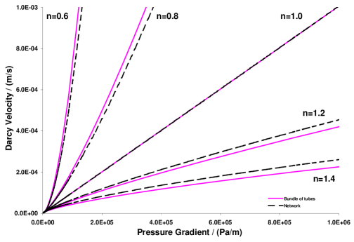
Figure 4.1: Comparison between the sand pack network ($x_{{}_{l}}=0.5$, $x_{{}_{u}}=0.95$, $K=102$ Darcy, $\phi=0.35$) and a bundle of tubes ($R=48.2\mu$m) for a Herschel-Bulkley fluid with $\tau_{o}=0.0$Pa and $C=0.1$Pa.sⁿ.

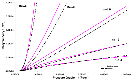
Figure 4.2: Comparison between the sand pack network ($x_{{}_{l}}=0.5$, $x_{{}_{u}}=0.95$, $K=102$ Darcy, $\phi=0.35$) and a bundle of tubes ($R=48.2\mu$m) for a Herschel-Bulkley fluid with $\tau_{o}=1.0$Pa and $C=0.1$Pa.sⁿ.

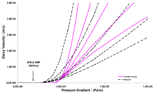
Figure 4.3: A magnified view of Figure (4.2) at the yield zone. The prediction of Invasion Percolation with Memory (IPM) and Path of Minimum Pressure (PMP) algorithms is indicated by the arrow.

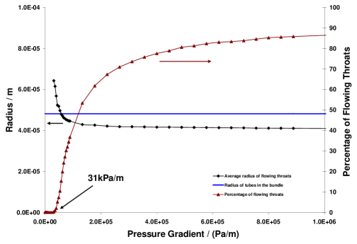
Figure 4.4: The radius of the bundle of tubes and the average radius of the non-blocked throats of the sand pack network, with their percentage of the total number of throats, as a function of pressure gradient for a Bingham fluid ($n=1.0$) with $\tau_{o}=1.0$Pa and $C=0.1$Pa.s.

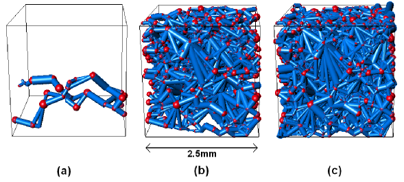
Figure 4.5: Visualization of the non-blocked elements of the sand pack network for a Bingham fluid ($n=1.0$) with $\tau_{o}=1.0$Pa and $C=0.1$Pa.s. The fraction of flowing elements is (a) 0.4% (b) 25% and (c) 69%.

4.1.2 Berea Sandstone Network

The physical and statistical details of this network can be found in Appendix G Table (G.2). This network is more tortuous and less homogeneous than the sand pack.

The comparison between the results of the Berea network simulation and the bundle of tubes for the case of a fluid with no yield-stress is displayed in Figure (4.6). By definition, the results of the network and the bundle of tubes are identical in the Newtonian case. There is a lack of symmetry between the shear-thinning and shear-thickening cases relative to the Newtonian case, i.e. while the network flow in the shear-thinning cases is considerably higher than the flow in the tubes, the difference between the two flows in the shear-thickening cases is tiny. The reason is the inhomogeneity of the Berea network coupled with the shear effects.

Another feature is that for the shear-thinning cases the average discrepancy between the two flows is much larger for the $n=0.6$ case than for $n=0.8$. The reason is that as the fluid becomes more shear-thinning by decreasing $n$, the disproportionality due to inhomogeneity in the contribution of the two groups of large and small throats is magnified resulting in the flow being carried out largely by a relatively small number of large throats. The opposite is observed in the two shear-thickening cases for the corresponding reason that shear-thickening smooths out the inhomogeneity because it damps the flow in the largest elements resulting in a more uniform flow throughout the network.

The comparison between the Berea network and the bundle of tubes for the case of a fluid with a yield-stress is displayed in Figure (4.7) beside a magnified view to the yield zone in Figure (4.8). As in the case of the sand pack network, the Berea network starts flowing before the tubes for the same reason that is the average radius of the non-blocked elements in the network at yield is larger than the radius of the tubes in the bundle, as can be seen in Figure (4.9).

For a Bingham plastic, the network flow exceeds the bundle of tubes flow at low pressure gradients, but the trend is reversed at high pressure gradients because some elements in the network are still blocked, as in the case of sand pack.

For the two shear-thinning cases, the general features of the network-bundle of tubes relation are similar to those in the case of fluid with no yield-stress. However, the discrepancy between the two flows is now larger especially at low pressure gradients. There are three factors affecting the network-bundle of tubes relation. The first is the shift because the network yields before the bundle of tubes. This factor dominates at low pressure gradients. The second is the inhomogeneity coupled with shear-thinning, as outlined in the case of sand pack. The third is the blocking of some network elements with the effect of reducing the total flow. The second and the third factors compete, especially at high pressure gradients, and they determine the network-bundle of tubes relation which can take any form depending on the network and fluid properties and the pressure gradient. In the current case, the graphs suggest that for the fluid with $n=0.6$ the second factor dominates, while for the fluid with $n=0.8$ the two factors have almost similar impact.

For the two shear-thickening cases, the network flow exceeds the bundle of tubes flow at the beginning as the network yields before the bundle, but this eventually is overturned as in the case of a Bingham fluid with enforcement by the shear-thickening effect which impedes the network flow and reduces it at high pressure gradients. Because the average radius of the non-blocked throats in the Berea network is greater than the radius of the tubes in the bundle for all pressure gradients, as seen in Figure (4.9), the fluid in the network will be subject to more shear-thickening than the fluid in the bundle. Unlike shear-thinning cases, the inhomogeneity coupled with shear effects and partial blocking of the network are now enforcing each other to deter the flow. Consequently, the discrepancy between the network and the bundle of tubes in the two cases, i.e. $n=1.2$ and $n=1.4$, is larger than that in the corresponding cases of a fluid with no yield-stress.

Finally, it should be remarked that the superiority of the sand pack results in comparison to the Berea can be regarded as a sign of good behavior for our network model. The reason is that it has been shown in previous studies that the capillary bundle model is better suited for describing porous media that are unconsolidated and have high permeability [91].

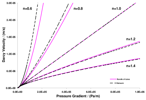
Figure 4.6: Comparison between Berea network ($x_{{}_{l}}=0.5$, $x_{{}_{u}}=0.95$, $K=3.15$ Darcy, $\phi=0.19$) and a bundle of tubes ($R=11.6\mu$m) for a Herschel-Bulkley fluid with $\tau_{o}=0.0$Pa and $C=0.1$Pa.sⁿ.

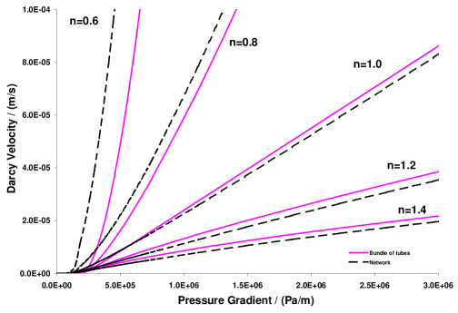
Figure 4.7: Comparison between Berea network ($x_{{}_{l}}=0.5$, $x_{{}_{u}}=0.95$, $K=3.15$ Darcy, $\phi=0.19$) and a bundle of tubes ($R=11.6\mu$m) for a Herschel-Bulkley fluid with $\tau_{o}=1.0$Pa and $C=0.1$Pa.sⁿ.

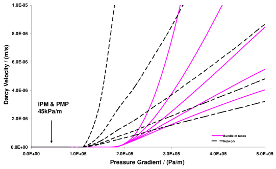
Figure 4.8: A magnified view of Figure (4.7) at the yield zone. The prediction of Invasion Percolation with Memory (IPM) and Path of Minimum Pressure (PMP) algorithms is indicated by the arrow.

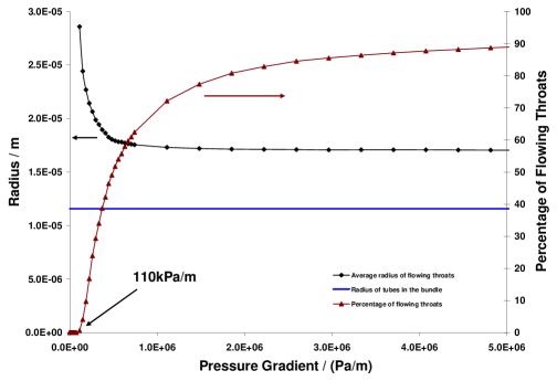
Figure 4.9: The radius of the bundle of tubes and the average radius of the non-blocked throats of the Berea network, with the percentage of the total number of throats, as a function of pressure gradient for a Bingham fluid ($n=1.0$) with $\tau_{o}=1.0$Pa and $C=0.1$Pa.s.

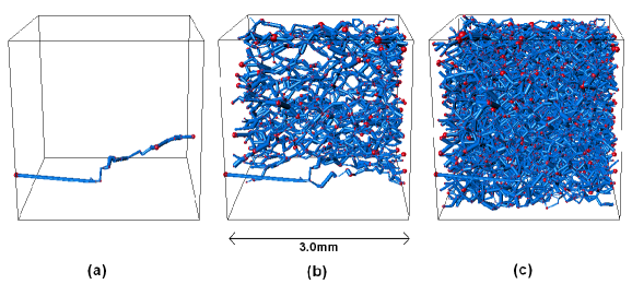
Figure 4.10: Visualization of the non-blocked elements of the Berea network for a Bingham fluid ($n=1.0$) with $\tau_{o}=1.0$Pa and $C=0.1$Pa.s. The fraction of flowing elements is (a) 0.1% (b) 9% and (c) 41%.

4.2 Random vs. Cubic Networks Comparison

In this section we present a brief comparison between a cubic network on one hand and each one of the sand pack and Berea networks on the other. In both cases, the cubic network was generated by “netgen” of Valvatne with a truncated Weibull distribution, which is the only distribution available in this code, subject to the two extreme limits for the throat radius and length of the corresponding random network. The truncated Weibull distribution of a variable $V$ with a minimum value $V_{min}$ and a maximum value $V_{max}$ is given, according to Valvatne [78], by

$$V=V_{min}+(V_{max}-V_{min})\,\left[-a\ln\{x(1-e^{-1/a})+e^{-1/a}\}\right]^{1/b}$$ (4.2)

where $a$ and $b$ are parameters defining the shape of the distribution and $x$ is a random number between 0 and 1. The values of $a$ and $b$ in each case were chosen to have a reasonable match to the corresponding random network distribution.

The cubic network has also been modified to have the same coordination number as the random network. Using “poreflow” of Valvatne [78] the cubic network was then tuned to match the permeability and porosity of the corresponding random network. The simulation results from our non-Newtonian code for a Herschel-Bulkley fluid with $C=0.1$Pa.sⁿ and $n=0.6,0.8,1.0,1.2,1.4$ for both cases of yield-free fluid ($\tau_{o}=0.0$Pa) and yield-stress fluid ($\tau_{o}=1.0$Pa) are presented in Figures (4.11-4.14).

As can be seen, the results match very well for the sand pack network with a yield-free fluid, as in Figure (4.11). For the sand pack with a yield-stress fluid, as in Figure (4.12), there is a shift between the two networks and the cubic flow lags behind the sand pack. This can be explained by the dependency of the network yield on the actual void space characteristics rather than the network bulk properties such as permeability and porosity.

For the Berea network, the match between the two networks is poor in both cases. For non-yield-stress fluids, as presented in Figure (4.13), the two networks match in the Newtonian case by definition. However, the match is poor for the non-Newtonian fluids. As for yield-stress fluids, seen in Figure (4.14), the divergence between the two networks in the shear-thinning cases is large with the cubic network underestimating the flow. Similarly for the Bingham fluid though the divergence is less serious. As for the two cases of shear-thickening, the two networks produce reasonably close predictions with the cubic network giving higher flow rate. Several interacting factors, like the ones presented in the random networks section, can explain this behavior. However, the general conclusion is that the non-Newtonian behavior in general depends on the actual void space characteristics rather than the network bulk properties. The inhomogeneity of the Berea network may also have aggravated the situation and exacerbated the shift.

It should be remarked that the cubic results in general depends on the cubic network realization as there is an element of randomness in the cubic network distributions during its generation. The dependency is more obvious in the case of yield-stress fluids as the yield of a network is highly dependent on the topology and geometry of the void space. Similar argument can be presented for the random networks since they are generated by simulating the geological processes by which the porous medium was formed.

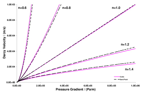
Figure 4.11: Comparison between the sand pack network ($x_{{}_{l}}=0.5$, $x_{{}_{u}}=0.95$, $K=102$ Darcy, $\phi=0.35$) and a cubic network having the same throat distribution, coordination number, permeability and porosity for a Herschel-Bulkley fluid with $\tau_{o}=0.0$Pa and $C=0.1$Pa.sⁿ.

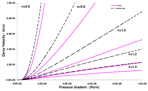
Figure 4.12: Comparison between the sand pack network ($x_{{}_{l}}=0.5$, $x_{{}_{u}}=0.95$, $K=102$ Darcy, $\phi=0.35$) and a cubic network having the same throat distribution, coordination number, permeability and porosity for a Herschel-Bulkley fluid with $\tau_{o}=1.0$Pa and $C=0.1$Pa.sⁿ.

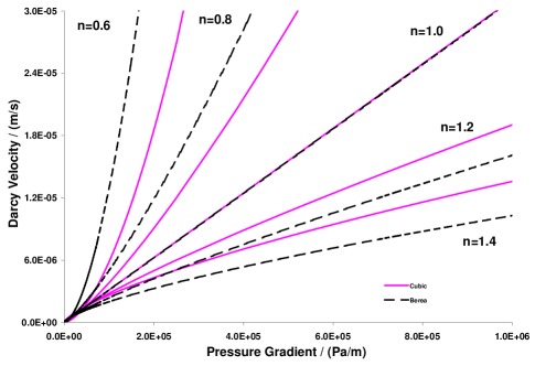
Figure 4.13: Comparison between the Berea network ($x_{{}_{l}}=0.5$, $x_{{}_{u}}=0.95$, $K=3.15$ Darcy, $\phi=0.19$) and a cubic network having the same throat distribution, coordination number, permeability and porosity for a Herschel-Bulkley fluid with $\tau_{o}=0.0$Pa and $C=0.1$Pa.sⁿ.

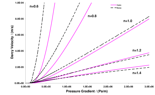
Figure 4.14: Comparison between the Berea network ($x_{{}_{l}}=0.5$, $x_{{}_{u}}=0.95$, $K=3.15$ Darcy, $\phi=0.19$) and a cubic network having the same throat distribution, coordination number, permeability and porosity for a Herschel-Bulkley fluid with $\tau_{o}=1.0$Pa and $C=0.1$Pa.sⁿ.

4.3 Bundle of Tubes vs. Experimental Data Comparison

To gain a better insight into the bundle of tubes model, which we used to carry a preliminary assessment to the random network model, we present in Figures (4.15) and (4.16) a comparison between the bundle of tubes model predictions and a sample of the Park’s Herschel-Bulkley experimental data that will be thoroughly discussed in Section (5.2.1). The bulk rheology of these data sets can be found in Table (5.3).

Although, the experimental data do not match well to the bundle of tubes model results, the agreement is good enough for such a crude model. A remarkable feature is the close similarity between the bundle of tubes curves seen in Figures (4.15) and (4.16) and the network curves seen in Figures (5.9) and (5.10). This should be expected since the network results are produced with a scaled version of the sand pack network, and as we observed in Section (4.1.1) there is a good match between the sand pack network and the bundle of tubes model.

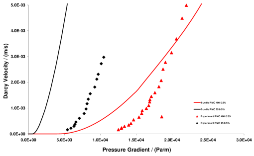
Figure 4.15: Sample of Park’s Herschel-Bulkley experimental data group for aqueous solutions of PMC 400 and PMC 25 flowing through a coarse packed bed of glass beads having $K=3413$ Darcy and $\phi=0.42$ alongside the results of a bundle of tubes with $R=255\mu$m.

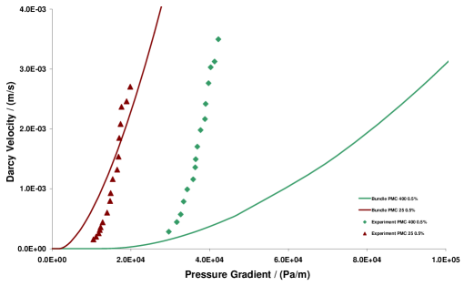
Figure 4.16: Sample of Park’s Herschel-Bulkley experimental data group for aqueous solutions of PMC 400 and PMC 25 flowing through a fine packed bed of glass beads having $K=366$ Darcy and $\phi=0.39$ alongside the results of a bundle of tubes with $R=87\mu$m.

Chapter 5 Experimental Validation for Ellis and Herschel-Bulkley Models

We implemented the Ellis and Herschel-Bulkley models in our non-Newtonian code using the analytical expressions for the volumetric flow rate, i.e. Equation (1.4) for Ellis and Equation (1.1.2) for Herschel-Bulkley. In this chapter, we will discuss the validation of our network model by the few complete experimental data collections that we found in the literature. In all the cases presented in this chapter, the sand pack network was used after scaling to match the permeability of the porous media used in the experiments. The reason for using the sand pack instead of Berea is that the sand pack is a better match, though not ideal, to the packed beds used in the experiments in terms of homogeneity and tortuosity. The length factor which we used to scale the networks is given by $\sqrt{\frac{K_{{}_{exp}}}{K_{{}_{net}}}}$ where $K_{{}_{exp}}$ is the permeability of the experimental pack and $K_{{}_{net}}$ is the permeability of the original network as obtained from Newtonian flow simulation.

5.1 Ellis Model

Three complete collections of experimental data found in the literature on Ellis fluid were investigated. Good agreement with the network model results was obtained in most cases.

5.1.1 Sadowski

In this collection [31], twenty complete data sets of ten aqueous polymeric solutions flowing through packed beds of lead shot or glass beads with various properties were investigated. The bulk rheology was given by Sadowski in his dissertation and is shown in Table (5.1) with the corresponding bed properties. The in situ experimental data was obtained from the relevant tables in the dissertation. The permeability of the beds, which is needed to scale our sand pack network, was obtained from the formula suggested by Sadowski, that is

$$K=\frac{D_{p}^{2}}{C^{{}^{\prime\prime}}}\frac{\epsilon^{3}}{(1-\epsilon)^{2}}$$ (5.1)

where $K$ is the absolute permeability of the bed, $D_{p}$ is the diameter of the bed particles, $\epsilon$ is the porosity and $C^{{}^{\prime\prime}}$ is a dimensionless constant assigned a value of 180 by Sadowski.

A sample of the simulation results, with the corresponding experimental data sets, is presented in Figures (5.1) and (5.2) as Darcy velocity versus pressure gradient, and Figures (5.3) and (5.4) as apparent viscosity versus Darcy velocity. As seen, the agreement between the experimental data and the network simulation is very good in most cases.

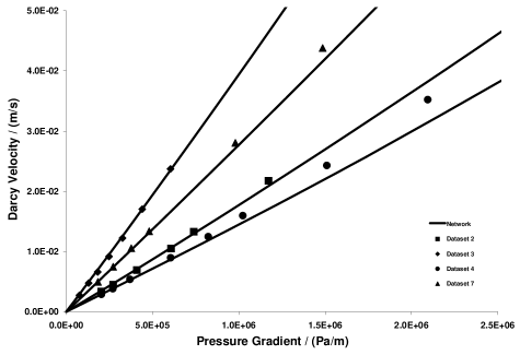
Figure 5.1: Sample of the Sadowski’s Ellis experimental data sets (2,3,4,7) for a number of solutions with various concentrations and different bed properties alongside the simulation results obtained with scaled sand pack networks having the same $K$ presented as $q$ vs. $|\nabla P|$.

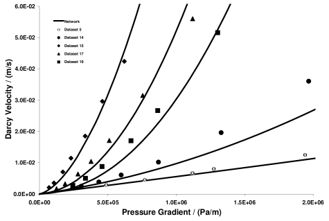
Figure 5.2: Sample of the Sadowski’s Ellis experimental data sets (5,14,15,17,19) for a number of solutions with various concentrations and different bed properties alongside the simulation results obtained with scaled sand pack networks having the same $K$ presented as $q$ vs. $|\nabla P|$.

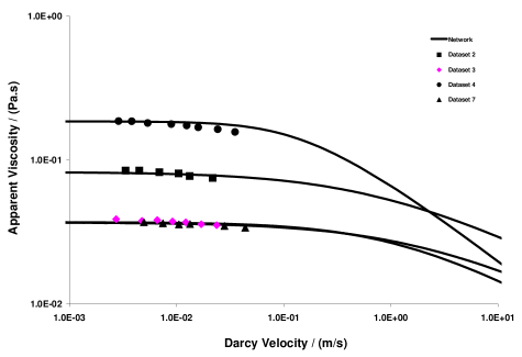
Figure 5.3: Sample of the Sadowski’s Ellis experimental data sets (2,3,4,7) for a number of solutions with various concentrations and different bed properties alongside the simulation results obtained with scaled sand pack networks having the same $K$ presented as $\mu_{a}$ vs. $q$.

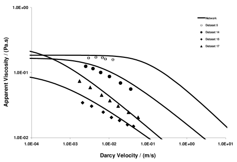
Figure 5.4: Sample of the Sadowski’s Ellis experimental data sets (5,14,15,17) for a number of solutions with various concentrations and different bed properties alongside the simulation results obtained with scaled sand pack networks having the same $K$ presented as $\mu_{a}$ vs. $q$.

	Fluid Properties				Bed Properties
Set	Solution	$\mu_{o}$ (Pa.s)	$\alpha$	$\tau_{{}_{1/2}}$ (Pa)	$K$ (m2)	$\phi$
1	18.5% Carbowax 20-M	0.0823	1.674	3216.0	3.80E-09	0.3690
2	18.5% Carbowax 20-M	0.0823	1.674	3216.0	1.39E-09	0.3812
3	14.0% Carbowax 20-M	0.0367	1.668	3741.0	1.38E-09	0.3807
4	6.0% Elvanol 72-51	0.1850	2.400	1025.0	2.63E-09	0.3833
5	6.0% Elvanol 72-51	0.1850	2.400	1025.0	1.02E-09	0.3816
6	6.0% Elvanol 72-51	0.1850	2.400	1025.0	3.93E-09	0.3720
7	3.9% Elvanol 72-51	0.0369	1.820	2764.0	9.96E-10	0.3795
8	1.4% Natrosol - 250G	0.0688	1.917	59.9	2.48E-09	0.3780
9	1.4% Natrosol - 250G	0.0688	1.917	59.9	1.01E-09	0.3808
10	1.4% Natrosol - 250G	0.0688	1.917	59.9	4.17E-09	0.3774
11	1.6% Natrosol - 250G	0.1064	1.971	59.1	2.57E-09	0.3814
12	1.6% Natrosol - 250G	0.1064	1.971	59.1	1.01E-09	0.3806
13	1.85% Natrosol - 250G	0.1670	2.006	60.5	3.91E-09	0.3717
14	1.85% Natrosol - 250G	0.1670	2.006	60.5	1.02E-09	0.3818
15	0.4% Natrosol - 250H	0.1000	1.811	2.2	1.02E-09	0.3818
16	0.4% Natrosol - 250H	0.1000	1.811	2.2	4.21E-09	0.3783
17	0.5% Natrosol - 250H	0.2500	2.055	3.5	1.03E-09	0.3824
18	0.5% Natrosol - 250H	0.2500	2.055	3.5	5.30E-09	0.3653
19	0.6% Natrosol - 250H	0.4000	2.168	5.2	1.07E-09	0.3862
20	0.6% Natrosol - 250H	0.4000	2.168	5.2	5.91E-09	0.3750

Table 5.1: The bulk rheology and bed properties of Sadowski’s Ellis experimental data.

5.1.2 Park

In this collection [32], four complete data sets on the flow of aqueous polyacrylamide solutions with different weight concentration in packed beds of glass beads were investigated. The bulk rheology was given by Park and is shown in Table (5.2). The in situ experimental data was obtained from the relevant tables in his dissertation. The permeability of the bed, which is needed to scale our sand pack network, was obtained from Equation (5.1), as suggested by Park, with the constant $C^{{}^{\prime\prime}}$ obtained from fitting his Newtonian flow data, as will be described in the Park’s Herschel-Bulkley experimental data section. The simulation results compared to the experimental data points are shown in Figure (5.5) as Darcy velocity versus pressure gradient, and Figure (5.6) as apparent viscosity versus Darcy velocity. As seen, the agreement in all cases is very good. The discrepancy observed in some cases in the high flow rate region is due apparently to the absence of a high shear Newtonian plateau in Ellis model.

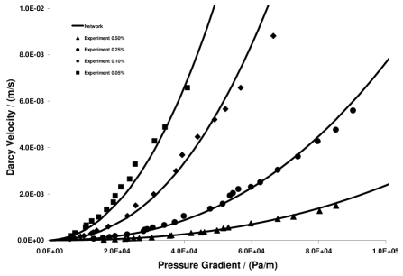
Figure 5.5: Park’s Ellis experimental data sets for polyacrylamide solutions with 0.50%, 0.25%, 0.10% and 0.05% weight concentration flowing through a coarse packed bed of glass beads having $K=3413$ Darcy and $\phi=0.42$ alongside the simulation results obtained with a scaled sand pack network having the same $K$ presented as $q$ vs. $|\nabla P|$.

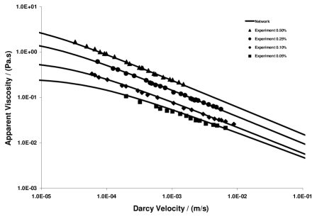
Figure 5.6: Park’s Ellis experimental data sets for polyacrylamide solutions with 0.50%, 0.25%, 0.10% and 0.05% weight concentration flowing through a coarse packed bed of glass beads having $K=3413$ Darcy and $\phi=0.42$ alongside the simulation results obtained with a scaled sand pack network having the same $K$ presented as $\mu_{a}$ vs. $q$.

Solution	$\mu_{o}$ (Pa.s)	$\alpha$	$\tau_{{}_{1/2}}$ (Pa)
0.50%	4.35213	2.4712	0.7185
0.25%	1.87862	2.4367	0.5310
0.10%	0.60870	2.3481	0.3920
0.05%	0.26026	2.1902	0.3390

Table 5.2: The bulk rheology of Park’s Ellis experimental data.

5.1.3 Balhoff

A complete data set for guar gum solution of 0.72 % concentration with Ellis parameters $\mu_{o}=2.672$ Pa.s, $\alpha=3.46$ and $\tau_{{}_{1/2}}=9.01$ Pa flowing through a packed bed of glass beads having $K=4.19\times 10^{-9}$ m² and $\phi=0.38$ was investigated. The bulk rheology was given by Balhoff in his dissertation [34] and the in situ experimental data was obtained from Balhoff by private communication.

The simulation results with the experimental data points are presented in Figure (5.7) as Darcy velocity versus pressure gradient, and Figure (5.8) as apparent viscosity versus Darcy velocity. As seen, the agreement is very good. Again, a discrepancy is observed in the high flow rate region because of the absence of a high-shear Newtonian plateau in the Ellis model.

Figure 5.7: Balhoff’s Ellis experimental data set for guar gum solution with 0.72% concentration flowing through a packed bed of glass beads having $K=4.19\times 10^{-9}$ m² and $\phi=0.38$ alongside the simulation results obtained with a scaled sand pack network having the same $K$ presented as $q$ vs. $|\nabla P|$.

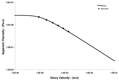
Figure 5.8: Balhoff’s Ellis experimental data set for guar gum solution with 0.72% concentration flowing through a packed bed of glass beads having $K=4.19\times 10^{-9}$ m² and $\phi=0.38$ alongside the simulation results obtained with a scaled sand pack network having the same $K$ presented as $\mu_{a}$ vs. $q$.

5.2 Herschel-Bulkley Model

Three complete collections of experimental data found in the literature on Herschel-Bulkley fluid were investigated. Limited agreement with the network model predictions was obtained.

5.2.1 Park

In this collection [32], eight complete data sets are presented. The fluid is an aqueous solution of Polymethylcellulose (PMC) with two different molecular weights, PMC 25 and PMC 400, each with concentration of 0.3% and 0.5% weight. For each of the four solutions, two packed beds of spherical uniform-in-size glass beads, coarse and fine, were used.

The in situ experimental data, alongside the fluids’ bulk rheology and the properties of the porous media, were tabulated in Park’s thesis. However, the permeability of the two beds, which is needed to scale our network, is missing. To overcome this difficulty, Darcy’s law was applied to the Newtonian flow results of the fine bed, as presented in Table M-1 in Park’s thesis [32], to extract the permeability of this bed from the slope of the best fit line to the data points. In his dissertation, Park presented the permeability relation of Equation (5.1) where $C^{{}^{\prime\prime}}$ is a dimensionless constant to be determined from experiment and have been assigned in the literature a value between 150 and 180 depending on the author. To find the permeability of the coarse bed, we obtained a value for $C^{{}^{\prime\prime}}$ from Equation (5.1) by substituting the permeability of the fine bed, with the other relevant parameters. This value ($\simeq 164$) was then substituted in the formula with the relevant parameters to obtain the permeability of the coarse bed.

We used our non-Newtonian code with two scaled sand pack networks and the bulk rheology presented in Table (5.3) to simulate the flow. The simulation results with the corresponding experimental data sets are presented in Figures (5.9) and (5.10). As seen, the predictions are poor. One possible reason is the high shear-thinning nature of the solutions, with $n$ between 0.57 and 0.66. This can produce a large discrepancy even for a small error in $n$. The failure to predict the threshold yield pressure is also noticeable. Retention and other similar phenomena may be ruled out as a possible cause for the higher experimental threshold yield pressure by the fact that the solutions, according to Park, were filtered to avoid gel formation.

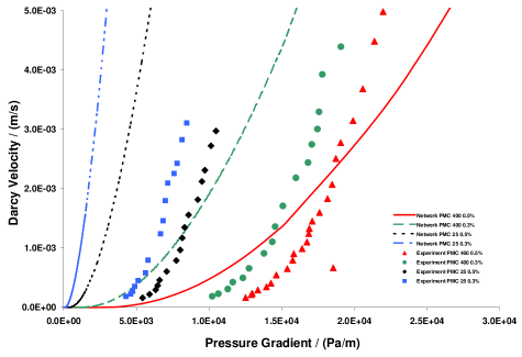
Figure 5.9: Park’s Herschel-Bulkley experimental data group for aqueous solutions of PMC 400 and PMC 25 with 0.5% and 0.3% weight concentration flowing through a coarse packed bed of glass beads having $K=3413$ Darcy and $\phi=0.42$ alongside the simulation results obtained with a scaled sand pack network having same $K$.

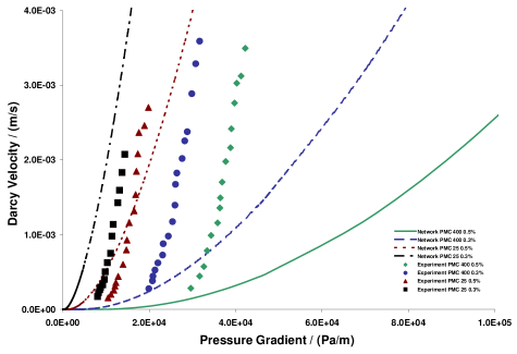
Figure 5.10: Park’s Herschel-Bulkley experimental data group for aqueous solutions of PMC 400 and PMC 25 with 0.5% and 0.3% weight concentration flowing through a fine packed bed of glass beads having $K=366$ Darcy and $\phi=0.39$ alongside the simulation results obtained with a scaled sand pack network having same $K$.

5.2.2 Al-Fariss and Pinder

In this collection [37], there are sixteen complete sets of data for waxy oils with the bulk and in situ rheologies. The porous media consist of two packed beds of sand having different dimensions, porosity, permeability and grain size. We used the bulk rheology given by the authors and extracted the in situ rheology from the relevant graphs. The bulk rheology and bed properties are given in Table (5.4).

The non-Newtonian code was used with two scaled sand pack networks and the bulk rheology to simulate the flow. A sample of the simulation results, with the corresponding in situ experimental data points, is shown in Figures (5.11) and (5.12). Analyzing the experimental and network results reveals that while the network behavior is consistent, considering the underlying bulk rheology, the experimental data exhibit an inconsistent pattern. This is evident when looking at the in situ behavior as a function of the bulk rheology which, in turn, is a function of temperature.

The sixteen data sets are divided into four groups. In each group the fluid and the porous medium are the same but the fluid temperature varies. On analyzing the in situ data, one can discover that there is no obvious correlation between the fluid properties and its temperature. An example is the 4.0% wax in Clarus B group where an increase in temperature from 14 ^∘C to 16 ^∘C results in a drop in the flow at high pressures rather than rise, opposite to what is expected from the general trend of the experimental data and the fact that the viscosity usually decreases on increasing the temperature, as the bulk rheology tells. One possibility is that in some cases the wax-oil mix may not be homogenous, so other physical phenomena such as wax precipitation took place. Such complex phenomena are accounted for neither in our model nor in the Al-Fariss and Pinder model. This might be inferred from the more consistent experimental results for the waxy crude oil.

It is noteworthy that the Al-Fariss and Pinder model failed to cope with these irregularities. As a result they arbitrarily modified the model parameters on case-by-case basis to fit the experimental data.

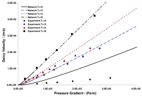
Figure 5.11: Al-Fariss and Pinder’s Herschel-Bulkley experimental data group for 2.5% wax in Clarus B oil flowing through a column of sand having $K=315$ Darcy and $\phi=0.36$ alongside the simulation results obtained with a scaled sand pack network having the same $K$ and $\phi$. The temperatures, T, are in ^∘C.

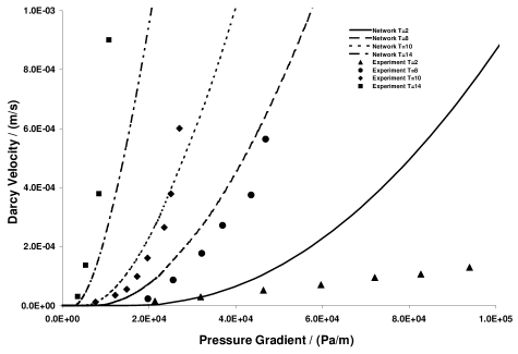
Figure 5.12: Al-Fariss and Pinder’s Herschel-Bulkley experimental data group for waxy crude oil flowing through a column of sand having $K=1580$ Darcy and $\phi=0.44$ alongside the simulation results obtained with a scaled sand pack network having the same $K$. The temperatures, T, are in ^∘C.

5.2.3 Chase and Dachavijit

In this collection [43], there are ten complete data sets for Bingham aqueous solutions of Carbopol 941 with concentration varying between 0.15 and 1.3 mass percent. The porous medium is a packed column of spherical glass beads having a narrow size distribution. The bulk rheology, which is extracted from a digitized image and given in Table (5.5), represents the actual experimental data points rather than the least square fitting suggested by the authors.

Our non-Newtonian code was used to simulate the flow of a Bingham fluid with the extracted bulk rheology through a scaled sand pack network. The scaling factor was chosen to have a permeability that produces a best fit to the most Newtonianlike data set, excluding the first data set with the lowest concentration due to a very large relative error and a lack of fit to the trend line.

The simulation results, with the corresponding in situ experimental data sets extracted from digitized images of the relevant graphs, are presented in Figures (5.13) and (5.14). The fit is good in most cases. The experimental data in some cases shows irregularities which may suggest large experimental errors or other physical phenomena, such as retention, taking place. This erratic behavior cannot fit a consistent pattern.

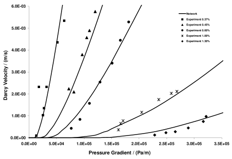
Figure 5.13: Network simulation results with the corresponding experimental data points of Chase and Dachavijit for a Bingham aqueous solution of Carbopol 941 with various concentrations (0.37%, 0.45%, 0.60%, 1.00% and 1.30%) flowing through a packed column of glass beads.

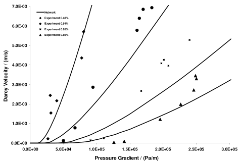
Figure 5.14: Network simulation results with the corresponding experimental data points of Chase and Dachavijit for a Bingham aqueous solution of Carbopol 941 with various concentrations (0.40%, 0.54%, 0.65% and 0.86%) flowing through a packed column of glass beads.

Solution	$C$ (Pa.sn)	$n$	$\tau_{o}$ (Pa)
0.50% PMC 400	0.116	0.57	0.535
0.30% PMC 400	0.059	0.61	0.250
0.50% PMC 25	0.021	0.63	0.072
0.30% PMC 25	0.009	0.66	0.018

Table 5.3: The bulk rheology of Park’s Herschel-Bulkley experimental data.

Fluid Properties					Bed Properties
Wax (%)	T (∘C)	$C$ (Pa.sn)	$n$	$\tau_{o}$ (Pa)	$K$ (m2)	$\phi$
2.5	10	0.675	0.89	0.605	3.15E-10	0.36
2.5	12	0.383	0.96	0.231	3.15E-10	0.36
2.5	14	0.300	0.96	0.142	3.15E-10	0.36
2.5	18	0.201	0.97	0.071	3.15E-10	0.36
4.0	12	1.222	0.77	3.362	3.15E-10	0.36
4.0	14	0.335	0.97	3.150	3.15E-10	0.36
4.0	16	0.461	0.88	1.636	3.15E-10	0.36
4.0	18	0.436	0.85	0.480	3.15E-10	0.36
4.0	20	0.285	0.90	0.196	3.15E-10	0.36
5.0	16	0.463	0.87	3.575	3.15E-10	0.36
5.0	18	0.568	0.80	2.650	3.15E-10	0.36
5.0	20	0.302	0.90	1.921	3.15E-10	0.36
Crude	2	0.673	0.54	2.106	1.58E-09	0.44
Crude	8	0.278	0.61	0.943	1.58E-09	0.44
Crude	10	0.127	0.70	0.676	1.58E-09	0.44
Crude	14	0.041	0.81	0.356	1.58E-09	0.44

Table 5.4: The bulk rheology and bed properties for the Herschel-Bulkley experimental data of Al-Fariss and Pinder.

Concentration (%)	C (Pa.s)	$\tau_{o}$ (Pa)
0.15	0.003	0.08
0.37	0.017	2.06
0.40	0.027	2.39
0.45	0.038	4.41
0.54	0.066	4.37
0.60	0.057	7.09
0.65	0.108	8.70
0.86	0.136	12.67
1.00	0.128	17.33
1.30	0.215	28.46

Table 5.5: The bulk rheology of Chase and Dachavijit experimental data for a Bingham fluid ($n=1.0$).

5.3 Assessing Ellis and Herschel-Bulkley Results

The experimental validation of Ellis model is generally good. What is remarkable is that this simple model was able to predict several experimental data sets without introducing any arbitrary factors. All we did is to use the bulk rheology and the bed properties as an input to the non-Newtonian code. In fact, these results were obtained with a scaled sand pack network which in most cases is not an ideal representation of the porous medium used. Also remarkable is the use of an analytical expression for the volumetric flow rate instead of an empirical one as done by Lopez [80, 81] in the case of the Carreau model.

Regarding the Herschel-Bulkley model, the experimental validation falls short of expectation. Nevertheless, even coming this close to the experimental data is a success, being aware of the level of sophistication of the model and the complexities of the three-dimensional networks, and considering the fact that the physics so far is relatively simple. Incorporating more physics in the model and using better void space description in the form of more realistic networks can improve the results.

However, it should be remarked that the complexity of the yield-stress phenomenon may be behind this relative failure of the Herschel-Bulkley model implementation. The flow of yield-stress fluids in porous media is apparently too complex to describe by a simple rheological model such as Herschel-Bulkley, too problematic to investigate by primitive experimental techniques and too difficult to model by the available tools of pore-scale modeling at the current level of sophistication. This impression is supported by the fact that much better results are obtained for non-yield-stress fluids, like Ellis  using the same tools and techniques. One major limitation of our network model with regard to the yield-stress fluids is that we use analytical expressions for cylindrical tubes based on the concept of equivalent radius $R_{eq}$ which we presented earlier. This is far from the reality as the void space is highly complex in shape. The result is that the yield condition for circular tube becomes invalid approximation to the actual yield condition for the pore space. The simplistic nature of the yield condition in porous media is highlighted by the fact that in almost all cases of disagreement between the network and the experimental results the network produced a lower yield value. Other limitations and difficulties associated with the yield-stress fluids in general, and hence affect our model, will be discussed in the next section.

In summary, yield-stress fluid results are extremely sensitive to how the fluid is characterized, how the void space is described and how the yield process is modeled. In the absence of a comprehensive and precise incorporation of all these factors in the modeling procedure, pore scale modeling of yield-stress fluids in porous media remains an inaccurate approximation that may not produce quantitatively sensible predictions.

Chapter 6 Yield-Stress Analysis

Yield-stress or viscoplastic fluids can sustain shear stresses, that is a certain amount of stress must be exceeded before the flow starts. So an ideal yield-stress fluid is a solid before yield and a fluid after. Accordingly, the viscosity of the substance changes from an infinite to a finite value. However, the physical situation suggests that it is more realistic to regard a yield-stress substance as a fluid whose viscosity as a function of applied stress has a discontinuity as it drops sharply from a very high value on exceeding a critical yield-stress.

There are many controversies and unsettled issues in the non-Newtonian literature about yield-stress phenomenon and yield-stress fluids. In fact, even the concept of a yield-stress has received much recent criticism, with evidence presented to suggest that most materials weakly yield or creep near zero strain rate. The supporting argument is that any material will flow provided that one waits long enough. These conceptual difficulties are supported by practical and experimental complications. For example, the value of the yield-stress for a particular fluid is difficult to measure consistently and it may vary by more than one order of magnitude depending on the measurement technique [6, 11, 92, 26].

Several constitutive equations to describe liquids with yield-stress are in use; the most popular ones are Bingham, Casson and Herschel-Bulkley. Some have suggested that the yield-stress values obtained via such models should be considered model parameters and not real material properties.

There are several difficulties in working with the yield-stress fluids and validating the experimental data. One difficulty is that the yield-stress value is usually obtained by extrapolating a plot of shear stress to zero shear rate [11, 33, 37, 34]. This extrapolation can result in a variety of values for yield-stress, depending on the distance from the shear stress axis experimentally accessible by the instrument used. The vast majority of yield-stress data reported results from such extrapolations, making most values in the literature instrument-dependent [11]. Another method used to measure yield-stress is by lowering the shear rate until the shear stress approaches a constant. This may be identified as the dynamic yield-stress [13]. The results obtained using these methods may not agree with the static yield-stress measured directly without disturbing the microstructure during the measurement. The latter seems more relevant for the flow initiation under gradual increase in pressure gradient as in the case of flow in porous media. Consequently, the accuracy of the predictions made using flow simulation models in conjunction with such experimental data is limited.

Another difficulty is that while in the case of pipe flow the yield-stress value is a property of the fluid, in the case of flow in porous media there are strong indications that in a number of situations it may depend on both the fluid and the porous medium itself [42, 93]. One possible explanation is that the yield-stress value may depend on the size and shape of the pore space when the polymer molecules become comparable in size to the void space. The implicit assumption that the yield-stress value at pore scale is the same as the yield value at bulk may not be self evident. This makes the predictions of the network models based on analytical solution to the flow in a single tube combined with the bulk rheology less accurate. When the duct size is small, as it is usually the case in porous media, flow of macromolecule solutions normally displays deviations from predictions based on corresponding viscometric data [12]. Consequently, the concept of equivalent radius $R_{eq}$, which is used in the network modeling, though is completely appropriate for the Newtonian flow and reasonably appropriate for the non-Newtonian with no yield-stress, seems inappropriate for yield-stress fluids as the yield depends on the actual shape of the void space rather than the equivalent radius and flow conductance.

In porous media, threshold yield pressure is expected to be directly proportional to the yield-stress of the fluid and inversely proportional to the porosity and permeability of the media [72]. A shortcoming of using continuum models, such as an extended Darcy’s law, to study the flow of yield-stress fluids in porous media is that these models are unable to correctly describe the network behavior at transition where the network is partly flowing. The reason is that according to these models the network is either fully blocked or fully flowing whereas in reality the network smoothly yields. For instance, these models predict for Bingham fluids a linear relationship between Darcy velocity and pressure gradient with an intercept at threshold yield gradient whereas our network model and that of others [45], supported by experimental evidence, predict a nonlinear behavior at transition stage [42]. Some authors have concluded that in a certain range the macroscopic flow rate of Bingham plastic in a network depends quadratically on the departure of the applied pressure difference from its minimum value [94]. Our network simulation results confirm this quadratic correlation. Samples of this behavior for the sand pack and Berea networks are given in Figures (6.1) and (6.2). As can be seen, the match between the network points and the least-square fitting quadratic curve is almost perfect in the case of the sand pack. For the Berea network the agreement is less obvious. A possible cause is the inhomogeneity of the Berea network which makes the flow less regular.

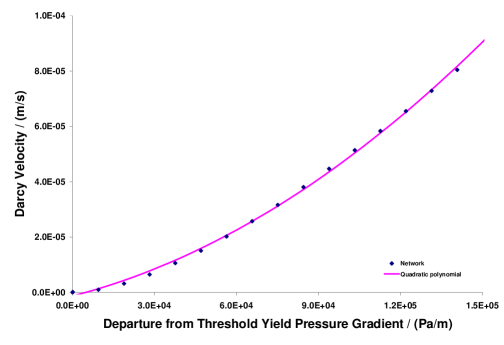
Figure 6.1: Comparison between the sand pack network simulation results for a Bingham fluid with $\tau_{o}=1.0$Pa and the least-square fitting quadratic $y=2.39\times 10^{-15}\,x^{2}+2.53\times 10^{-10}\,x-1.26\times 10^{-6}$.

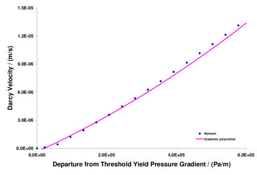
Figure 6.2: Comparison between the Berea network simulation results for a Bingham fluid with $\tau_{o}=1.0$Pa and the least-square fitting quadratic $y=1.00\times 10^{-17}\,x^{2}+1.69\times 10^{-11}\,x-3.54\times 10^{-7}$.

6.1 Predicting the Yield Pressure of a Network

Predicting the threshold yield pressure of a yield-stress fluid in porous media in its simplest form may be regarded as a special case of the more general problem of finding the threshold conduction path in disordered media consisting of elements with randomly distributed thresholds. This problem was analyzed by Roux and Hansen [95, 96] in the context of studying the conduction of an electric network of diodes by considering two different cases, one in which the path is directed (no backtracking) and one in which it is not. They suggested that the minimum overall threshold potential difference across the network is akin to a percolation threshold and studied its dependence on the lattice size.

Kharabaf and Yortsos [95] noticed that a firm connection of the lattice-threshold problem to percolation appears to be lacking and the relation of the Minimum Threshold Path (MTP) to the minimum path of percolation, if it indeed exists, is not self-evident. They presented a new algorithm, Invasion Percolation with Memory (IPM), for the construction of the MTP, based on which its properties can be studied. This algorithm will be closely examined later on.

In a series of studies on generation and mobilization of foam in porous media, Rossen et al  [97, 98] analyzed the threshold yield pressure using percolation theory concepts and suggested a simple percolation model. In this model, the percolation cluster is first found, then the MTP was approximated as a subset of this cluster that samples those bonds with the smallest individual thresholds [94].

Chen et al [94] elucidated the Invasion Percolation with Memory method of Kharabaf. They further extended this method to incorporate dynamic effects due to the viscous friction following the onset of mobilization.

It is tempting to consider the yield-stress fluid behavior in porous media as a percolation phenomenon to be analyzed by the classical percolation theory. However, three reasons, at least, may suggest otherwise:

1. The conventional percolation models can be applied only if the conducting elements are homogeneous, i.e. it is assumed in these models that the intrinsic property of all elements in the network are equal. However, this assumption cannot be justified for most kinds of media where the elements vary in their conduction and yield properties. Therefore, to apply percolation principles, a generalization to the conventional percolation theory is needed as suggested by Selyakov and Kadet [99].

2. The network elements cannot yield independently as a spanning path bridging the inlet to the outlet is a necessary condition for yield. This contradicts the percolation theory assumption that the elements conduct independently.

3. The pure percolation approach ignores the dynamic aspects of the pressure field, that is a stable pressure configuration is a necessary condition which may not coincide with the simple percolation requirement. The percolation condition, as required by the classic percolation theory, determines the stage at which the network starts flowing according to the intrinsic properties of its elements as an ensemble of conducting bonds regardless of the dynamic aspects introduced by the external pressure field.

In this thesis, two approaches to predict the network threshold yield pressure are presented and carefully examined: the Invasion Percolation with Memory of Kharabaf, and the Path of Minimum Pressure which is a novel approach that we propose. Both approaches are implemented in our three-dimensional network model of non-Newtonian code and the results are extracted. An extensive analysis is conducted to compare the prediction and performance of these approaches and relate their results to the network threshold yield pressure as obtained from flow simulation.

6.1.1 Invasion Percolation with Memory (IPM)

The IPM is a way for finding the inlet-to-outlet path that minimizes the sum of the values of a property assigned to the individual elements of the network, and hence finding this minimum. For a yield-stress fluid, this reduces to finding the inlet-to-outlet path that minimizes the yield pressure. The yield pressure of this path is taken as the network threshold yield pressure. An algorithm to find the threshold yield pressure according to IPM is outlined below:

1. Initially, the nodes on the inlet are considered to be sources and the nodes on the outlet and inside are targets. The inlet nodes are assigned a pressure value of 0.0. According to the IPM, a source cannot be a target and vice versa, i.e. they are disjoint sets and remain so in all stages.

2. Starting from the source nodes, a step forward is made in which the yield front advances one bond from a single source node. The condition for choosing this step is that the sum of the source pressure plus the yield pressure of the bond connecting the source to the target node is the minimum of all similar sums from the source nodes to the possible target nodes. This sum is assigned to the target node.

3. This target node loses its status as a target and obtains the status of a source.

4. The last two steps are repeated until the outlet is reached, i.e. when the target is an outlet node. The pressure assigned to this target node is regarded as the yield pressure of the network.

This algorithm was implemented in our non-Newtonian flow simulation code as outlined below:

1. Two boolean vectors and one double vector each of size $N$, where $N$ is the number of the network nodes, are used. The boolean vectors are used to store the status of the nodes, one for the sources and one for the targets. The double vector is used for storing the yield pressure assigned to the nodes. The vectors are initialized as explained already.

2. A loop over all sources is started in which the sum of the pressure value of the source node plus the threshold yield pressure of the bond connecting the source node to one of the possible target nodes is computed. This is applied to all targets connected to all sources.

3. The minimum of these sums is assigned to the respective target node. This target node is added to the source list and removed from the target list.

4. The last two steps are repeated until the respective target node is verified as an outlet node. The pressure assigned to the target node in the last loop is the network threshold yield pressure.

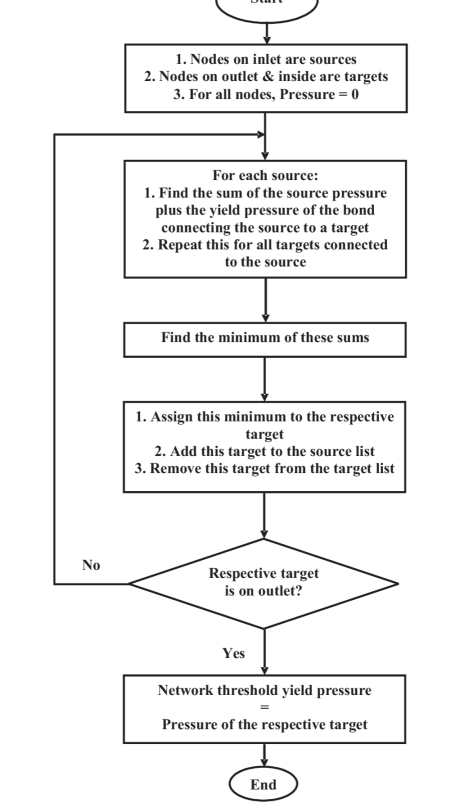
Figure 6.3: Flowchart of the Invasion Percolation with Memory (IPM) algorithm.

A flowchart of the IPM algorithm is given in Figure (6.3).

As implemented, the memory requirement for a network with $N$ nodes is 10$N$ bytes which is a trivial cost even for a large network. However, the CPU time for a medium-size network is considerable and expected to rise sharply with increasing size of the network. A sample of the IPM data is presented in Table (6.1) and Table (6.2) for the sand pack and Berea networks respectively, and in Table (6.3) and Table (6.4) for their cubic equivalents which are described in Section (4.3).

6.1.2 Path of Minimum Pressure (PMP)

This is a novel approach that we developed. It is based on a similar assumption to that upon which the IPM is based, that is the network threshold yield pressure is the minimum sum of the threshold yield pressures of the individual elements of all possible paths from the inlet to the outlet. However, it is computationally different and is more efficient than the IPM in terms of the CPU time and memory.

According to the PMP, to find the threshold yield pressure of a network:

1. All possible paths of serially-connected bonds from inlet to outlet are inspected. We impose a condition on the spanning path that there is no flow component opposite to the pressure gradient across the network in any part of the path, i.e. backtracking is not allowed.

2. For each path, the threshold yield pressure of each bond is computed and the sum of these pressures is found.

3. The network threshold yield pressure is taken as the minimum of these sums.

Despite its conceptual simplicity, the computational aspects of this approach for a three-dimensional topologically-complex network is formidable even for a relatively small network. It is highly demanding in terms of memory and CPU time. However, the algorithm was implemented in an efficient way. In fact, the algorithm was implemented in three different forms producing identical results but varying in their memory and CPU time requirements. The form outlined below is the slowest one in terms of CPU time but the most efficient in terms of memory:

1. A double vector of size $N$, where $N$ is the number of the network nodes, is used to store the yield pressure assigned to the nodes. The nodes on the inlet are initialized with zero pressure while the remaining nodes are initialized with infinite pressure (very high value).

2. A source is an inlet or an inside node with a finite pressure while a target is a node connected to a source through a single bond with the condition that the spatial coordinate of the target in the direction of the pressure gradient across the network is higher than the spatial coordinate of the source.

3. Looping over all sources, the threshold yield pressure of each bond connecting a source to a target is computed and the sum of this yield pressure plus the pressure of the source node is found. The minimum of this sum and the current yield pressure of the target node is assigned to the target node.

4. The loop in the last step is repeated until a stable state is reached when no target node changes its pressure during looping over all sources.

5. A loop over all outlet nodes is used to find the minimum pressure assigned to the outlet nodes. This pressure is taken as the network threshold yield pressure.

The PMP algorithm is graphically presented in a flow chart in Figure (6.4).

For a network with $N$ nodes the memory requirement is 8$N$ bytes which is still insignificant even for a large network. The CPU time is trivial even for a relatively large network and is expected to rise almost linearly with the size of the network. A sample of the PMP data is presented in Tables (6.1), (6.2), (6.3) and (6.4).

6.1.3 Analyzing IPM and PMP

As implemented in our non-Newtonian code, the two methods are very efficient in terms of memory requirement especially the PMP. The PMP is also very efficient in terms of CPU time. This is not the case with the IPM which is time-demanding compared to the PMP, as can be seen in Tables (6.1), (6.2), (6.3) and (6.4). So, the PMP is superior to the IPM in performance.

The two methods are used to investigate the threshold yield pressure of various slices of the sand pack and Berea networks and their cubic equivalent with different location and width, including the whole width, to obtain different networks with various characteristics. A sample of the results is presented in Tables (6.1), (6.2), (6.3) and (6.4).

It is noticeable that in most cases the IPM and PMP predict much lower threshold yield pressures than the network as obtained from solving the pressure field across the network in the flow simulation, as described in Section (3.1), particularly for the Berea network. The explanation is that both algorithms are based on the assumption that the threshold yield pressure of serially-connected bonds is the sum of their yield pressures. This assumption can be challenged by the fact that the pressure gradient across the ensemble should reach the threshold yield gradient for the bottleneck of the ensemble if yield should occur. Moreover the IPM and PMP disregard the global pressure field which can communicate with the internal nodes of the serially-connected ensemble as it is part of a network and not an isolated collection of bonds. It is not obvious that the IPM and PMP condition should agree with the requirement of a stable and mathematically consistent pressure filed as defined in Section (3.1). Such an agreement should be regarded as an extremely unlikely coincident. The static nature of the IPM and PMP is behind this failure, that is their predictions are based on the intrinsic properties of the network irrespective of the dynamic aspects introduced by the pressure field. Good predictions can be made only if the network is considered as a dynamic entity.

Several techniques were employed to investigate the divergence between the IPM and PMP predictions and the solver results. One of these techniques is to inspect the yield path at threshold when using the solver to find the pressure field. The results were conclusive; that is at the network yield point all elements in the path have already reached their yield pressure. In particular, there is a single element, a bottleneck, that is exactly at its threshold yield pressure. This confirms the reliability of the network model as it is functioning in line with the design. Beyond this, no significance should be attached to this as a novel science.

One way of assessing the results is to estimate the average throat size very roughly when flow starts in a yield-stress fluid by applying the percolation theory, as discussed by Rossen and Mamun [98], then comparing this to the average throat size as found from the pressure solver and from the IPM and PMP. However, we did not follow this line of investigation because we do not believe that network yield is a percolation phenomenon. Furthermore, the non-Newtonian code in its current state has no percolation capability.

In most cases of the random networks the predictions of the IPM and PMP agree. However, when they disagree the PMP gives a higher value of yield pressure. The reason is that backtracking is allowed in IPM but not in PMP. When the actual path of minimum sum has a backward component, which is not allowed by the PMP, the alternative path of next minimum sum with no backtracking is more restrictive and hence has a higher yield pressure value. This explanation is supported by the predictions of the regular networks where the two methods produce identical results as backtracking is less likely to occur in a cubic network since it involves a more tortuous and restrictive path with more than one connecting bond.

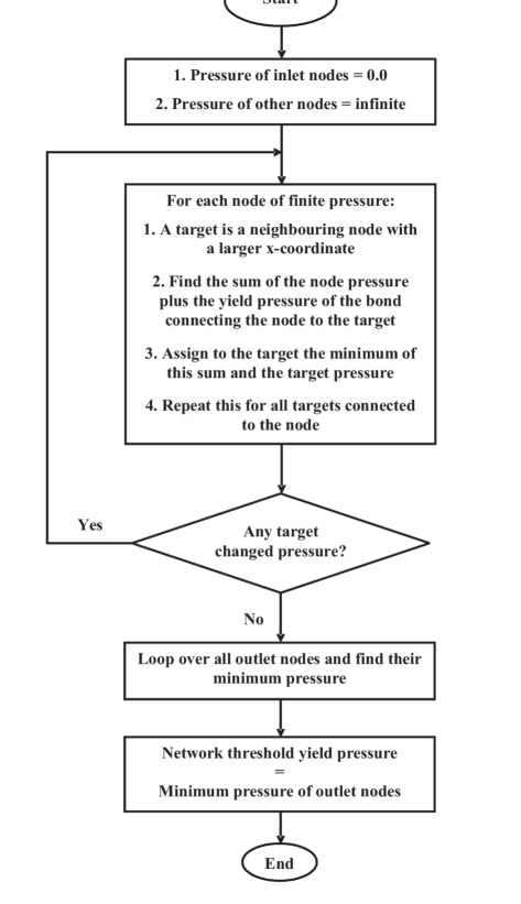
Figure 6.4: Flowchart of the Path of Minimum Pressure (PMP) algorithm.

Table 6.1: Comparison between IPM and PMP for various slices of the sand pack.

	Boundary		Py (Pa)			Iterations		Time (s)
No.	$x_{{}_{l}}$	$x_{{}_{u}}$	Network	IPM	PMP	IPM	PMP	IPM	PMP
1	0.0	1.0	80.94	53.81	54.92	2774	14	2.77	0.17
2	0.0	0.9	71.25	49.85	51.13	2542	11	2.47	0.13
3	0.0	0.8	61.14	43.96	44.08	2219	10	2.09	0.11
4	0.0	0.7	56.34	38.47	38.74	1917	9	1.75	0.08
5	0.0	0.6	51.76	32.93	33.77	1607	10	1.42	0.08
6	0.0	0.5	29.06	21.52	21.52	1048	9	0.84	0.06
7	0.0	0.4	24.24	18.45	18.45	897	9	0.69	0.05
8	0.0	0.3	18.45	12.97	12.97	622	7	0.44	0.03
9	0.1	1.0	69.75	47.67	48.78	2323	12	2.41	0.16
10	0.1	0.9	60.24	43.71	44.70	2084	9	2.14	0.09
11	0.1	0.8	49.53	37.82	37.94	1756	9	1.75	0.09
12	0.1	0.7	43.68	32.27	32.27	1471	9	1.42	0.09
13	0.1	0.6	39.72	26.64	26.64	1176	10	1.08	0.08
14	0.1	0.5	18.82	15.39	15.39	602	9	0.52	0.06
15	0.1	0.4	14.40	12.32	12.32	448	8	0.38	0.03
16	0.2	1.0	53.81	43.26	43.86	2060	12	2.08	0.14
17	0.2	0.9	46.44	39.30	40.19	1843	10	1.86	0.09
18	0.2	0.8	37.13	30.27	30.27	1372	9	1.33	0.08
19	0.2	0.7	37.84	24.28	24.28	1044	9	0.94	0.06
20	0.2	0.6	29.32	19.96	19.96	811	8	0.69	0.05
21	0.2	0.5	21.26	10.98	10.98	416	7	0.33	0.03
22	0.3	1.0	53.19	37.85	37.85	1727	11	1.75	0.09
23	0.3	0.9	45.64	33.56	33.56	1508	9	1.50	0.08
24	0.3	0.8	37.36	23.42	23.42	1006	7	0.95	0.05
25	0.3	0.7	28.43	17.43	17.43	672	7	0.58	0.05
26	0.3	0.6	19.09	10.94	10.94	355	7	0.27	0.03
27	0.4	1.0	47.23	30.46	30.96	1378	11	1.42	0.09
28	0.4	0.9	28.35	24.44	24.44	1062	8	1.08	0.06
29	0.4	0.8	24.28	15.82	15.82	623	8	0.59	0.05
30	0.4	0.7	10.00	9.83	9.83	301	6	0.24	0.03
31	0.5	1.0	36.25	24.68	24.68	1119	8	1.08	0.05
32	0.5	0.9	28.20	19.25	19.25	821	7	0.77	0.03
33	0.5	0.8	20.85	13.71	13.71	528	7	0.47	0.03

Note: this data is for a Bingham fluid ($n=1.0$) with $\tau_{o}=1.0$Pa. The PMP is implemented in three forms. The “Iterations” and “time” data is for the slowest but the least memory demanding form. The machine used is a Pentium 3.4 GHz processor workstation.

Table 6.2: Comparison between IPM and PMP for various slices of Berea.

	Boundary		Py (Pa)			Iterations		Time (s)
No.	$x_{{}_{l}}$	$x_{{}_{u}}$	Network	IPM	PMP	IPM	PMP	IPM	PMP
1	0.0	1.0	331.49	121.68	121.68	8729	29	20.31	1.11
2	0.0	0.9	251.20	102.98	104.46	7242	26	17.50	0.89
3	0.0	0.8	235.15	84.55	87.51	5759	24	13.02	0.72
4	0.0	0.7	148.47	62.32	62.32	3968	21	8.39	0.53
5	0.0	0.6	115.80	43.24	43.24	2311	18	3.94	0.38
6	0.0	0.5	59.49	27.34	27.34	1146	17	1.25	0.30
7	0.0	0.4	23.13	8.14	8.14	361	18	0.31	0.25
8	0.0	0.3	3.92	3.72	3.72	265	12	0.14	0.11
9	0.1	1.0	283.88	119.38	119.38	8402	31	19.56	1.13
10	0.1	0.9	208.97	100.67	102.15	7002	26	16.14	0.81
11	0.1	0.8	189.73	82.24	84.23	5575	22	12.49	0.61
12	0.1	0.7	128.55	60.02	60.02	3876	20	8.02	0.45
13	0.1	0.6	98.56	40.93	40.93	2417	16	4.64	0.30
14	0.1	0.5	37.81	25.04	25.04	1270	15	2.05	0.24
15	0.1	0.4	28.52	22.02	22.02	1073	21	1.66	0.36
16	0.2	1.0	295.77	110.33	115.60	7424	27	21.77	0.88
17	0.2	0.9	222.84	94.58	95.48	6228	22	13.67	0.61
18	0.2	0.8	191.51	72.05	72.05	4589	20	9.77	0.47
19	0.2	0.7	147.06	58.60	58.60	3605	18	7.34	0.34
20	0.2	0.6	82.05	39.52	39.52	2237	15	4.09	0.23
21	0.2	0.5	29.57	23.62	23.62	1150	11	1.80	0.13
22	0.3	1.0	295.95	96.73	102.00	6223	21	13.19	0.61
23	0.3	0.9	219.45	80.97	81.88	5076	21	10.49	0.52
24	0.3	0.8	171.16	58.45	58.45	3460	17	6.77	0.34
25	0.3	0.7	126.21	48.02	48.02	2723	15	5.05	0.23
26	0.3	0.6	56.09	34.52	34.52	1856	12	3.09	0.16
27	0.4	1.0	214.73	79.42	84.69	4923	22	9.92	0.56
28	0.4	0.9	149.53	63.67	64.58	3787	17	7.50	0.36
29	0.4	0.8	106.15	41.14	41.14	2227	14	3.99	0.25
30	0.4	0.7	60.82	30.71	30.71	1530	13	2.45	0.17
31	0.5	1.0	125.88	67.61	67.61	4211	19	8.69	0.38
32	0.5	0.9	94.17	54.47	54.49	3267	15	6.53	0.24
33	0.5	0.8	83.00	31.94	31.94	1711	12	3.13	0.14

Note: this data is for a Bingham fluid ($n=1.0$) with $\tau_{o}=1.0$Pa. The PMP is implemented in three forms. The “Iterations” and “time” data is for the slowest but the least memory demanding form. The machine used is a Pentium 3.4 GHz processor workstation.

Table 6.3: Comparison between IPM and PMP for various slices of a cubic network with similar properties to the sand pack.

	Boundary		Py (Pa)			Iterations		Time (s)
No.	$x_{{}_{l}}$	$x_{{}_{u}}$	Network	IPM	PMP	IPM	PMP	IPM	PMP
1	0.0	1.0	108.13	64.73	64.73	2860	9	1.39	0.14
2	0.0	0.9	81.72	53.94	53.94	2381	7	1.16	0.11
3	0.0	0.8	81.58	46.06	46.06	2006	7	0.97	0.09
4	0.0	0.7	62.99	39.05	39.05	1678	6	0.81	0.06
5	0.0	0.6	53.14	32.90	32.90	1401	6	0.67	0.05
6	0.0	0.5	40.20	27.50	27.50	1147	5	0.53	0.05
7	0.0	0.4	31.97	22.22	22.22	912	5	0.42	0.03
8	0.0	0.3	28.70	18.32	18.32	745	5	0.34	0.03
9	0.1	1.0	86.28	55.75	55.75	2422	9	1.19	0.14
10	0.1	0.9	63.74	44.95	44.95	1946	7	0.97	0.09
11	0.1	0.8	62.52	37.07	37.07	1568	7	0.77	0.08
12	0.1	0.7	42.70	30.07	30.07	1247	5	0.59	0.05
13	0.1	0.6	34.64	23.92	23.92	979	5	0.47	0.05
14	0.1	0.5	27.78	18.52	18.52	732	5	0.34	0.03
15	0.1	0.4	19.81	13.24	13.24	496	4	0.23	0.02
16	0.2	1.0	90.10	48.19	48.19	2200	5	1.08	0.08
17	0.2	0.9	73.98	39.92	39.92	1834	5	0.88	0.05
18	0.2	0.8	61.36	32.21	32.21	1475	5	0.72	0.05
19	0.2	0.7	39.98	25.40	25.40	1158	5	0.55	0.05
20	0.2	0.6	30.63	19.24	19.24	878	5	0.41	0.05
21	0.2	0.5	21.62	13.84	13.84	650	4	0.30	0.02
22	0.3	1.0	47.09	44.33	44.33	1879	5	0.91	0.06
23	0.3	0.9	37.88	35.73	35.73	1484	5	0.72	0.05
24	0.3	0.8	30.84	25.88	25.88	1045	5	0.50	0.03
25	0.3	0.7	24.86	20.62	20.62	794	5	0.38	0.03
26	0.3	0.6	17.87	14.65	14.65	528	4	0.25	0.02
27	0.4	1.0	45.45	37.15	37.15	1657	5	0.81	0.05
28	0.4	0.9	36.02	29.30	29.30	1302	5	0.63	0.03
29	0.4	0.8	26.66	20.42	20.42	914	5	0.44	0.03
30	0.4	0.7	19.90	15.16	15.16	675	4	0.33	0.02
31	0.5	1.0	52.31	30.35	30.35	1392	6	0.67	0.05
32	0.5	0.9	37.67	22.08	22.08	1016	6	0.47	0.05
33	0.5	0.8	21.99	16.33	16.33	764	5	0.36	0.03

Note: this data is for a Bingham fluid ($n=1.0$) with $\tau_{o}=1.0$Pa. The PMP is implemented in three forms. The “Iterations” and “time” data is for the slowest but the least memory demanding form. The machine used is a dual core 2.4 GHz processor workstation.

Table 6.4: Comparison between IPM and PMP for various slices of a cubic network with similar properties to Berea.

	Boundary		Py (Pa)			Iterations		Time (s)
No.	$x_{{}_{l}}$	$x_{{}_{u}}$	Network	IPM	PMP	IPM	PMP	IPM	PMP
1	0.0	1.0	128.46	100.13	100.13	10366	10	10.03	0.47
2	0.0	0.9	113.82	89.34	89.34	9188	9	8.89	0.38
3	0.0	0.8	100.77	81.07	81.07	8348	9	8.08	0.34
4	0.0	0.7	87.36	69.89	69.89	7167	8	6.91	0.28
5	0.0	0.6	75.21	58.59	58.59	5963	9	5.80	0.28
6	0.0	0.5	61.25	47.31	47.31	4747	7	4.45	0.17
7	0.0	0.4	50.22	37.11	37.11	3703	7	3.49	0.14
8	0.0	0.3	36.63	25.10	25.10	2429	6	2.25	0.09
9	0.1	1.0	111.99	88.24	88.24	8958	10	8.64	0.42
10	0.1	0.9	98.19	77.45	77.45	7762	10	7.38	0.38
11	0.1	0.8	86.46	65.83	65.83	6543	9	6.24	0.30
12	0.1	0.7	71.83	54.06	54.06	5309	8	5.00	0.23
13	0.1	0.6	58.74	45.49	45.49	4405	9	4.16	0.22
14	0.1	0.5	46.35	34.40	34.40	3216	7	3.03	0.13
15	0.1	0.4	34.56	24.20	24.20	2166	7	1.97	0.09
16	0.2	1.0	112.66	76.32	76.32	7742	9	7.34	0.36
17	0.2	0.9	96.83	65.57	65.57	6577	9	6.17	0.30
18	0.2	0.8	82.38	56.60	56.60	5615	8	5.27	0.24
19	0.2	0.7	68.62	44.65	44.65	4369	7	4.06	0.17
20	0.2	0.6	51.78	35.40	35.40	3398	8	3.13	0.17
21	0.2	0.5	36.82	25.56	25.56	2358	6	2.11	0.08
22	0.3	1.0	98.13	63.93	63.93	6576	8	6.25	0.28
23	0.3	0.9	82.63	53.18	53.18	5403	8	5.06	0.23
24	0.3	0.8	69.09	45.16	45.16	4557	8	4.27	0.19
25	0.3	0.7	53.13	34.73	34.73	3445	6	3.20	0.13
26	0.3	0.6	39.52	25.51	25.51	2503	7	2.28	0.11
27	0.4	1.0	138.82	52.26	52.26	5468	9	5.16	0.28
28	0.4	0.9	107.95	41.47	41.47	4259	7	3.94	0.17
29	0.4	0.8	71.37	33.20	33.20	3412	7	3.16	0.14
30	0.4	0.7	35.52	22.02	22.02	2223	6	2.02	0.09
31	0.5	1.0	74.88	46.07	46.07	4847	8	4.59	0.20
32	0.5	0.9	56.75	35.28	35.28	3683	7	3.44	0.16
33	0.5	0.8	41.24	24.59	24.59	2551	7	2.34	0.11

Note: this data is for a Bingham fluid ($n=1.0$) with $\tau_{o}=1.0$Pa. The PMP is implemented in three forms. The “Iterations” and “time” data is for the slowest but the least memory demanding form. The machine used is a dual core 2.4 GHz processor workstation.

Chapter 7 Viscoelasticity

Viscoelastic substances exhibit a dual nature of behavior by showing signs of both viscous fluids and elastic solids. In its most simple form, viscoelasticity can be modeled by combining Newton’s law for viscous fluids (stress $\propto$ rate of strain) with Hook’s law for elastic solids (stress $\propto$ strain), as given by the original Maxwell model and extended by the Convected Maxwell models for the nonlinear viscoelastic fluids. Although this idealization predicts several basic viscoelastic phenomena, it does so only qualitatively [18].

The behavior of viscoelastic fluids is drastically different from that of Newtonian and inelastic non-Newtonian fluids. This includes the presence of normal stresses in shear flows, sensitivity to deformation type, and memory effects such as stress relaxation and time-dependent viscosity. These features underlie the observed peculiar viscoelastic phenomena such as rod-climbing (Weissenberg effect), die swell and open-channel siphon [27, 18]. Most viscoelastic fluids exhibit shear-thinning and an elongational viscosity that is both strain and extensional strain rate dependent, in contrast to Newtonian fluids where the elongational viscosity is constant [27].

The behavior of viscoelastic fluids at any time is dependent on their recent deformation history, that is they possess a fading memory of their past. Indeed a material that has no memory cannot be elastic, since it has no way of remembering its original shape. Consequently, an ideal viscoelastic fluid should behave as an elastic solid in sufficiently rapid deformations and as a Newtonian liquid in sufficiently slow deformations. The justification is that the larger the strain rate, the more strain is imposed on the sample within the memory span of the fluid [27, 6, 18].

Many materials are viscoelastic but at different time scales that may not be reached. Dependent on the time scale of the flow, viscoelastic materials mainly show viscous or elastic behavior. The particular response of a sample in a given experiment depends on the time scale of the experiment in relation to a natural time of the material. Thus, if the experiment is relatively slow, the sample will appear to be viscous rather than elastic, whereas, if the experiment is relatively fast, it will appear to be elastic rather than viscous. At intermediate time scales mixed viscoelastic response is observed. Therefore the concept of a natural time of a material is important in characterizing the material as viscous or elastic. The ratio between the material time scale and the time scale of the flow is indicated by a non-dimensional number: the Deborah or the Weissenberg number [5, 100].

A common feature of viscoelastic fluids is stress relaxation after a sudden shearing displacement where stress overshoots to a maximum then starts decreasing exponentially and eventually settles to a steady state value. This phenomenon also takes place on cessation of steady shear flow where stress decays over a finite measurable length of time. This reveals that viscoelastic fluids are able to store and release energy in contrast to inelastic fluids which react instantaneously to the imposed deformation [6, 17, 18].

A defining characteristic of viscoelastic materials associated with stress relaxation is the relaxation time which may be defined as the time required for the shear stress in a simple shear flow to return to zero under constant strain condition. Hence for a Hookean elastic solid the relaxation time is infinite, while for a Newtonian fluid the relaxation of the stress is immediate and the relaxation time is zero. Relaxation times which are infinite or zero are never realized in reality as they correspond to the mathematical idealization of Hookean elastic solids and Newtonian liquids. In practice, stress relaxation after the imposition of constant strain condition takes place over some finite non-zero time interval [3].

The complexity of viscoelasticity is phenomenal and the subject is notorious for being extremely difficult and challenging. The constitutive equations for viscoelastic fluids are much too complex to be treated in a general manner. Further complications arise from the confusion created by the presence of other phenomena such as wall effects and polymer-wall interactions, and these appear to be system specific. Therefore, it is doubtful that a general fluid model capable of predicting all the flow responses of viscoelastic system with enough mathematical simplicity or tractability can emerge in the foreseeable future [50, 17, 101]. Understandably, despite the huge amount of literature composed in the last few decades on this subject, almost all these studies have investigated very simple cases in which substantial simplifications have been made using basic viscoelastic models.

In the last few decades, a general consensus has emerged that in the flow of viscoelastic fluids through porous media elastic effects should arise, though their precise nature is unknown or controversial. In porous media, viscoelastic effects can be important in certain cases. When they are, the actual pressure gradient will exceed the purely viscous gradient beyond a critical flow rate, as observed by several investigators. The normal stresses of high molecular polymer solutions can explain in part the high flow resistances encountered during viscoelastic flow through porous media. It is argued that the very high normal stress differences and Trouton ratios associated with polymeric fluids will produce increasing values of apparent viscosity when flow channels in the porous medium are of rapidly changing cross section.

Important aspects of non-Newtonian flow in general and viscoelastic flow in particular through porous media are still presenting serious challenge for modeling and quantification. There are intrinsic difficulties of characterizing non-Newtonian effects in the flow of polymer solutions and the complexities of the local geometry of the porous medium which give rise to a complex and pore-space-dependent flow field in which shear and extension coexist in various proportions that cannot be quantified. Flows through porous media cannot be classified as pure shear flows as the converging-diverging passages impose a predominantly extensional flow fields especially at high flow rates. Moreover, the extension viscosity of many non-Newtonian fluids increases dramatically with the extension rate. As a consequence, the relationship between the pressure drop and flow rate very often do not follow the observed Newtonian and inelastic non-Newtonian trend. Further complication arises from the fact that for complex fluids the stress depends not only on whether the flow is a shearing, extensional, or mixed type, but also on the whole history of the velocity gradient [49, 102, 70, 103, 66, 13].

7.1 Important Aspects for Flow in Porous Media

Strong experimental evidence indicates that the flow of viscoelastic fluids through packed beds can exhibit rapid increases in the pressure drop, or an increase in the apparent viscosity, above that expected for a comparable purely viscous fluid. This increase has been attributed to the extensional nature of the flow field in the pores caused by the successive expansions and contractions that a fluid element experiences as it traverses the pore space. Even though the flow field at pore level is not an ideal extensional flow due to the presence of shear and rotation, the increase in flow resistance is referred to as an extension thickening effect [104, 103, 54, 90].

There are two major interrelated aspects that have strong impact on the flow through porous media. These are extensional flow and converging-diverging geometry.

7.1.1 Extensional Flow

One complexity in the flow in general and through porous media in particular usually arises from the coexistence of shear and extensional components; sometimes with the added complication of inertia. Pure shear or elongational flow is very much the exception in practical situations, especially in the flow through porous media. By far the most common situation is for mixed flow to occur where deformation rates have components parallel and perpendicular to the principal flow direction. In such flows, the elongational components may be associated with the converging-diverging flow paths [5, 46].

A general consensus has emerged recently that the flow through packed beds has a substantial extensional component and typical polymer solutions exhibit strain hardening in extension, which is mainly responsible for the reported dramatic increases in pressure drop. Thus in principle the shear viscosity alone is inadequate to explain the observed excessive pressure gradients. One is therefore interested to know the relative importance of elastic and viscous effects or equivalently the relationship between normal and shear stresses for different shear rates [11, 101, 17].

Elongational flow is fundamentally different from shear, the material property characterizing the flow is not the viscosity, but the elongational viscosity. The behavior of the extensional viscosity function is very often qualitatively different from that of the shear viscosity function. For example, highly elastic polymer solutions that possess a viscosity which decreases monotonically in shear often exhibit an extensional viscosity that increases dramatically with strain rate. Thus, while the shear viscosity is shear-thinning  the extensional viscosity is extension thickening. A fluid for which the extension viscosity increases with increasing elongation rate is said to be tension-thickening, whilst, if it decreases with increasing elongation rate it is said to be tension-thinning [13, 5, 100].

An extensional or elongational flow is one in which fluid elements are subjected to extensions and compressions without being rotated or sheared. The study of the extensional flow in general as a relevant variable has only received attention in the last few decades with the realization that extensional flow is of significant relevance in many practical situations. Moreover, non-Newtonian elastic liquids often exhibit dramatically different extensional flow characteristics from Newtonian liquids. Before that, rheology was largely dominated by shear flow. The historical convention of matching only shear flow data with theoretical predictions in constitutive modeling may have to be rethought in those areas of interest where there is a large extensional contribution. Extensional flow experiments can be viewed as providing critical tests for any proposed constitutive equations [13, 17, 5, 105].

The elongation or extension viscosity $\mu_{x}$, also called Trouton viscosity, is defined as the ratio of tensile stress and rate of elongation under condition of steady flow when both these quantities attain constant values. Mathematically, it is given by

$$\mu_{x}=\frac{\tau_{E}}{\dot{\varepsilon}}$$ (7.1)

where $\tau_{E}$ ($=\tau_{11}-\tau_{22}$) is the normal stress difference and $\dot{\varepsilon}$ is the elongation rate. The stress $\tau_{11}$ is in the direction of the elongation while $\tau_{22}$ is in a direction perpendicular to the elongation [106, 100, 5].

Polymeric fluids show a non-constant elongational viscosity in steady and unsteady elongational flow. In general, it is a function of the extensional strain rate, just as the shear viscosity is a function of shear rate. However, the behavior of the extensional viscosity function is frequently qualitatively different from that of the shear viscosity [13, 5].

It is generally agreed that it is far more difficult to measure extensional viscosity than shear viscosity. There is therefore a gulf between the strong desire to measure extensional viscosity and the likely expectation of its fulfilment [5, 18]. A major difficulty that hinders the progress in this field is that it is difficult to achieve steady elongational flow and quantify it precisely. Despite the fact that many techniques have been developed for measuring the elongational flow properties, so far these techniques failed to produce consistent outcome as they generate results which can differ by several orders of magnitude. This indicates that these results are dependent on the method and instrument of measurement. This is highlighted by the view that the extensional viscometers provide measurements of an extensional viscosity rather than the extensional viscosity. The situation is made more complex by the fact that it is almost impossible to generate a pure extensional flow since a shear component is always present in real flow situations. This makes the measurements doubtful and inconclusive [6, 11, 2, 66].

For Newtonian and purely viscous inelastic non-Newtonian fluids the elongational viscosity is a constant that only depends on the type of elongational deformation. Moreover, the viscosity measured in a shearing flow can be used to predict the stress in other types of deformation. For example, in a simple uniaxial elongational flow of a Newtonian fluid the following relationship is satisfied

$$\mu_{x}=3\mu_{o}$$ (7.2)

For viscoelastic fluids the flow behavior is more complex and the extensional viscosity, like the shear viscosity, depends on both the strain rate and the time following the onset of straining. The rheological behavior of a complex fluid in extension is often very different from that in shear. Polymers usually have extremely high extensional viscosities which can be orders of magnitude higher than those expected on the basis of Newtonian theory. Moreover, the extensional viscosities of elastic polymer solutions can be thousands of times greater than the shear viscosities. To measure the departure of the ratio of extensional to shear viscosity from its Newtonian behavior, the rheologists have introduced what is known as the Trouton ratio usually defined as

$$Tr=\frac{\mu_{x}(\dot{\varepsilon})}{\mu_{s}(\sqrt{3}\dot{\varepsilon})}$$ (7.3)

For elastic liquids, the Trouton ratio is expected to be always greater than or equal to 3, with the value 3 only attained at vanishingly small strain rates. These liquids are known for having very high Trouton ratios which can be as high as l0⁴. This behavior has to be expected especially when the fluid combines shear-thinning with tension-thickening. However, it should be remarked that even for the fluids that show tension-thinning behavior the associated Trouton ratios usually increase with strain rate and are still significantly in excess of the inelastic value of three [89, 3, 107, 18, 13, 105, 5].

Figures (7.1) and (7.2) compare the elongational viscosity to the shear viscosity at isothermal condition for a typical viscoelastic fluid at various extension and shear rates. As seen in Figure (7.1), the shear viscosity curve can be divided into three regions. For low-shear rates, compared to the time scale of the fluid, the viscosity is approximately constant. It then equals the so-called zero-shear-rate viscosity. After this initial plateau the viscosity rapidly decreases with increasing shear-rate. This behavior is shear-thinning. However, there are some materials for which the reverse behavior is observed, that is the viscosity increases with shear rate giving rise to shear-thickening. For high shear rates the viscosity often approximates a constant value again. The constant viscosity extremes at low and high shear rates are known as the lower and upper Newtonian plateau, respectively [6, 18, 5, 100].

In Figure (7.2) the typical behavior of the elongational viscosity, $\mu_{x}$, of a viscoelastic fluid as a function of elongation rate, $\dot{\varepsilon}$, has been depicted. As seen, the elongational viscosity curve can be divided into three regions. At low elongation rates the elongational viscosity approaches a constant value known as the zero-elongation-rate elongational viscosity, which is three times the zero-shear-rate viscosity, just as for a Newtonian fluid. For somewhat larger elongation rates the elongational viscosity increases with increasing elongation rate until a maximum constant value is reached. If the elongation rate is increased once more the elongational viscosity may decrease again. A fluid for which $\mu_{x}$ increases with increasing $\dot{\varepsilon}$ is said to be tension-thickening, whilst if $\mu_{x}$ decreases with increasing $\dot{\varepsilon}$ it is said to be tension-thinning. It should be remarked that two polymeric liquids which may have essentially the same behavior in shear can show a different response in extension [100, 3, 89, 5, 13, 6].

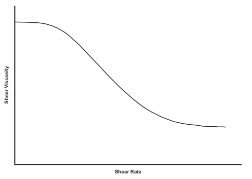
Figure 7.1: Typical behavior of shear viscosity $\mu_{s}$ as a function of shear rate $\dot{\gamma}$ in shear flow on a log-log scale.

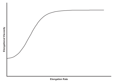
Figure 7.2: Typical behavior of elongational viscosity $\mu_{x}$ as a function of elongation rate $\dot{\varepsilon}$ in extensional flow on a log-log scale.

7.1.2 Converging-Diverging Geometry

An important aspect that characterizes the flow in porous media and makes it distinct from bulk is the presence of converging-diverging flow paths. This geometric factor significantly affects the flow and accentuate elastic responses. Several arguments have been presented in the literature to explain the effect of converging-diverging geometry on the flow behavior.

One argument is that viscoelastic flow in porous media differs from that of Newtonian flow, primarily because the converging-diverging nature of flow in porous media gives rise to normal stresses which are not solely proportional to the local shear rate. As the elastic nature of the fluid becomes more pronounced, an increase in flow resistance in excess of that due to purely shearing forces occurs [51]. A second argument is that in a pure shear flow the velocity gradient is perpendicular to the flow direction and the axial velocity is only a function of the radial coordinate, while in an elongational flow a velocity gradient in the flow direction exists and the axial velocity is a function of the axial coordinate. Any geometry which involves a diameter change will generate a flow field with elongational characteristics. Therefore the flow field in porous media is complex and involves both shear and elongational components [89]. A third argument suggests that elastic effects are expected in the flow through porous media because of the acceleration and deceleration of the fluid in the interstices of the bed upon entering and leaving individual pores [52, 33].

Despite this diversity, there is a general consensus that in porous media the converging-diverging nature of the flow paths brings out both the extensional and shear properties of the fluid. The principal mode of deformation to which a material element is subjected as the flow converges into a constriction involves both a shearing of the material element and a stretching or elongation in the direction of flow, while in the diverging portion the flow involves both shearing and compression. The actual channel geometry determines the ratio of shearing to extensional contributions. In many realistic situations involving viscoelastic flows the extensional contribution is the most important of the two modes. As porous media flow involves elongational flow components, the coil-stretch phenomenon can also take place. Consequently, a suitable model pore geometry is one having converging and diverging sections which can reproduce the elongational nature of the flow, a feature that is not exhibited by straight capillary tubes [49, 17, 89, 55, 90].

For long time, the straight capillary tube has been the conventional model for porous media and packed beds. Despite the general success of this model with the Newtonian and inelastic non-Newtonian flow, its failure with elastic flow was remarkable. To redress the flaws of this model, the undulating tube and converging-diverging channel were proposed in order to include the elastic character of the flow. Various corrugated tube models with different simple geometries have been used as a first step to model the effect of converging-diverging geometry on the flow of viscoelastic fluids in porous media (e.g. [49, 54, 108]). Those geometries include conically shaped sections, sinusoidal corrugation and abrupt expansions and contractions. Similarly, a bundle of converging-diverging tubes forms a better model for a porous medium in viscoelastic flow than the normally used bundle of straight capillary tubes, as the presence of diameter variations makes it possible to account for elongational contributions.

Many investigators have attempted to capture the role of the successive converging-diverging character of packed bed flow by numerically solving the flow equations in conduits of periodically varying cross sections. Different opinions on the success of these models can be found in the literature. Some of these are presented in the literature review [89, 17, 51, 101, 90, 109] in Chapter (2). With regards to modeling viscoelastic flow in regular or random networks of converging-diverging capillaries, very little work has been done.

7.2 Viscoelastic Effects in Porous Media

In packed bed flows, the main manifestation of steady-state viscoelastic effects is the excess pressure drop or dilatancy behavior in different flow regimes above what is accounted for by shear viscosity of the flowing liquid. Qualitatively, this behavior has been attributed to memory effects. Another explanation is that it is due to extensional flow. However, both explanations are valid and justified as long as the flow regime is considered. It should be remarked that the geometry of the porous media must be taken into account when considering elastic responses [101, 52].

It is generally agreed that the flow of viscoelastic fluids in packed beds results in a greater pressure drop than that which can be ascribed to the shear-rate-dependent viscosity. Fluids which exhibit elasticity deviate from viscous flow above some critical velocity in porous flow. At low flow rates, the pressure drop is determined largely by shear viscosity, and the viscosity and elasticity are approximately the same as in bulk. As the flow rate is gradually increased, viscoelastic effects begin to appear in various flow regimes. Consequently, the in situ rheological characteristics become significantly different from those in bulk rheology as the elasticity dramatically increases showing strong dilatant behavior [11, 52, 101].

Although experimental evidence for viscoelastic effects is convincing, an equally convincing theoretical analysis is not available. The general argument is that when the fluid suffers a significant deformation in a time comparable to the relaxation time of the fluid, elastic effects become important. When the pressure drop is plotted against a suitably defined Deborah or Weissenberg number, beyond a critical value of the Deborah number, the pressure drop increases rapidly [50, 11].

The complexity of the viscoelastic flow in porous media is aggravated by the possible occurrence of other non-viscoelastic phenomena which have similar effects as viscoelasticity. These phenomena include adsorption of the polymers on the capillary walls, mechanical retention and partial pore blockage. All these effects also lead to pressure drops well in excess to that expected from the shear viscosity levels. Consequently, the interpretation of many observed effects is confused and controversial. Some authors may interpret some observations in terms of partial pore blockage whereas others insist on non-Newtonian effects including viscoelasticity as an explanation. However, none of these have proved to be completely satisfactory. Yet, no one can rule out the possibility of simultaneous occurrence of these elastic and inelastic phenomena with further complication and confusion. A disturbing fact is the observation made by several researchers, e.g. Sadowski [31], that reproducible results could be obtained only in constant flow rate experiments because at constant pressure drop the velocity kept decreasing. This kind of observation indicates deposition of polymer on the solid surface by one mechanism or another, and cast doubt on some explanations which involve elasticity. At constant flow rate the increased pressure drop seems to provide the necessary force to keep a reproducible portion of the flow channels open [102, 110, 10, 101].

There are three principal viscoelastic effects that have to be accounted for in viscoelasticity investigation: transient time-dependence, steady-state time-dependence and dilatancy at high flow rates.

7.2.1 Transient Time-Dependence

Transient or time-dependent viscoelastic behavior has been observed in bulk on the startup and cessation of processes involving the displacement of viscoelastic materials, and on a sudden change of rate or reversal in the direction of deformation. During these transient states, there are frequently overshoots and undershoots in stress as a function of time which scale with strain. However, if the fluid is strained at a constant rate, these transients die out in the course of time, and the stress approaches a steady-state value that depends only on the strain rate. For example, under initial flow conditions stresses can reach magnitudes which are substantially more important than their steady-state values, whereas the relaxation on a sudden cessation of strain can vary substantially in various circumstances [11, 13, 25, 6, 111].

Transient responses are usually investigated in the context of bulk rheology, despite the fact that there is no available theory that can quantitatively predict this behavior. As a consequence of this limitation to bulk, the literature of viscoelastic flow in porous media is almost entirely dedicated to the steady-state situation with hardly any work on the in situ time-dependent viscoelastic flows. However, transient behavior should be expected in similar situations in the flow through porous media. One reason for this gap is the absence of a proper theoretical structure and the experimental difficulties associated with these flows in situ. Another possible explanation is that the in situ transient flows may have less important practical applications.

7.2.2 Steady-State Time-Dependence

By this, we mean the effects that may arise in the steady-state flow due to time dependency, as the time-dependence characteristics of the viscoelastic material must have an impact on the steady-state behavior. Therefore, elastic effects should be expected during steady-state flow in porous media because of the time-dependence nature of the flow at the pore level [52].

Depending on the time scale of the flow, viscoelastic materials may show viscous or elastic behavior. The particular response in a given process depends on the time scale of the process in relation to a natural time of the material [100, 5]. With regard to this time-scale dependency of viscoelastic flow process at pore scale, it has been suggested that the fluid relaxation time and the rate of elongation or contraction that occurs as the fluid flows through a channel or pore with varying cross-sectional area should be used to represent viscoelastic behavior [49, 53].

Sadowski and Bird [9] analyzed the viscometric flow problem in a long straight circular tube and argued that in such a flow no time-dependent elastic effects are expected. However, in a porous medium elastic effects may occur. As the fluid moves through a tortuous channel in the porous medium, it encounters a capriciously changing cross-section. If the fluid relaxation time is small with respect to the transit time through a contraction or expansion in a tortuous channel, the fluid will readjust to the changing flow conditions and no elastic effects would be observed. If, on the other hand, the fluid relaxation time is large with respect to the time to go through a contraction or expansion, then the fluid will not accommodate and elastic effects will be observed in the form of an extra pressure drop or an increase in the apparent viscosity. Thus the concept of a ratio of characteristic times emerges as an ordering parameter in non-Newtonian flow through porous media. This indicates the importance of the ratio of the natural time of a fluid to the duration time of a process, i.e. the residence time of the fluid element in a process [10]. It should be remarked that this formulation relies on an approximate dual-nature ordering scheme and is valid for some systems and flow regimes. More elaborate formulation will be given in the next paragraph in conjunction with the intermediate plateau phenomenon.

One of the steady-state viscoelastic phenomena observed in the flow through porous media and can be qualified as a time-dependent effect, among other possibilities such as retention, is the intermediate plateau at medium flow rates as demonstrated in Figure (1.3). A possible explanation is that at low flow rates before the appearance of the intermediate plateau the fluid behaves inelastically like any typical shear-thinning fluid. This implies that in the low flow regime viscoelastic effects are negligible as the fluid is able to respond to its local state of deformation essentially instantly, that is it does not remember its earlier configurations or deformation rates and hence behaves as a purely viscous fluid. As the flow rate increases above a threshold, a point will be reached at which the solid-like characteristics of viscoelastic materials begin to appear in the form of an increased pressure drop or increased apparent viscosity as the time of process becomes comparable to the natural time of fluid, and hence a plateau is observed. At higher flow rates the process time is short compared to the natural time of the fluid and hence the fluid has no time to react as the fluid is not an ideal elastic solid which reacts instantaneously. Since the precess time is very short, no overshoot will occur at the tube constriction as a measurable finite time is needed for the overshoot to take place. The result is that no increase in the pressure drop will be observed in this flow regime and the normal shear-thinning behavior is resumed with the eventual high flow rate plateau [49, 112].

It is worth mentioning that Dauben and Menzie [102] have discussed a similar issue in conjunction with the effect of diverging-converging geometry on the flow through porous media. They argued that the process of expansion and contraction repeated many times may account in part for the high pressure drops encountered during viscoelastic flow in porous media. The fluid relaxation time combined with the flow velocity determines the response of the viscoelastic fluid in the suggested diverging-converging model. Accordingly, it is possible that if the relaxation time is long enough or the fluid velocity high enough the fluid can pass through the large opening before it has had time to respond to a stress change imposed at the opening entrance, and hence the fluid would behave more as a viscous and less like a viscoelastic.

7.2.3 Dilatancy at High Flow Rates

The third distinctive feature of viscoelastic flow is the dilatant behavior in the form of excess pressure losses at high flow rates as schematically depicted in Figure (1.4). Certain polymeric solutions which exhibit shear-thinning behavior in a viscometric flow seem to exhibit a shear-thickening response under appropriate conditions of flow through porous media. Under high flow conditions through porous media, abnormal increases in flow resistance which resemble a shear-thickening response have been observed in flow experiments involving a variety of dilute to moderately concentrated solutions of high molecular weight polymers [10, 46].

This phenomenon can be attributed to stretch-thickening behavior due to the dominance of extensional over shear flow. At high flow rates strong extensional flow effects do occur and the extensional viscosity rises very steeply with increasing extension rate. As a result, the non-shear terms become much larger than the shear terms. For Newtonian fluids, the extensional viscosity is just three times the shear viscosity. However, for viscoelastic fluids the shear and extensional viscosities often behave oppositely, that is while the shear viscosity is generally a decreasing function of the shear rate, the extensional viscosity increases as the extension rate is increased. The consequence is that the pressure drop will be governed by the extension thickening behavior and the apparent viscosity rises sharply. Other possibilities such as physical retention are less likely to take place at these high flow rates [55, 66].

Finally a question may arise that why dilatancy at high flow rates occurs in some situations while intermediate plateau occurs in others? It seems that the combined effect of the fluid and porous media properties and the nature of the process is behind this difference.

7.3 Bautista-Manero Model

This is a relatively simple model that combines the Oldroyd-B constitutive equation for viscoelasticity (1.13) and the Fredrickson’s kinetic equation for flow-induced structural changes usually associated with thixotropy. The model requires six parameters that have physical significance and can be estimated from rheological measurements. These parameters are the low and high shear rate viscosities, the elastic modulus, the relaxation time, and two other constants describing the build up and break down of viscosity.

The kinetic equation of Fredrickson that accounts for the destruction and construction of structure is given by

$$\frac{\textrm{d}\mu}{\textrm{d}t}=\frac{\mu}{\lambda}\left(1-\frac{\mu}{\mu_{o}}\right)+k\mu\left(1-\frac{\mu}{\mu_{\infty}}\right)\mbox{\boldmath{$\tau$}}:\mbox{\boldmath{$\dot{\gamma}$}}$$ (7.4)

where $\mu$ is the non-Newtonian viscosity, $t$ is the time of deformation, $\lambda$ is the relaxation time upon the cessation of steady flow, $\mu_{o}$ and $\mu_{\infty}$ are the viscosities at zero and infinite shear rates respectively, $k$ is a parameter that is related to a critical stress value below which the material exhibits primary creep, $\tau$ is the stress tensor and $\dot{\gamma}$ is the rate of strain tensor. In this model, $\lambda$ is a structural relaxation time, whereas $k$ is a kinetic constant for structure break down. The elastic modulus $G_{o}$ is related to these parameters by $G_{o}=\mu/\lambda$ [111, 113, 114, 8].

Bautista-Manero model was originally proposed for the rheology of worm-like micellar solutions which usually have an upper Newtonian plateau, and show strong signs of shear-thinning. The model, which incorporates shear-thinning, elasticity and thixotropy, can be used to describe the complex rheological behavior of viscoelastic systems that also exhibit thixotropy and rheopexy under shear flow. The model predicts creep behavior, stress relaxation and the presence of thixotropic loops when the sample is subjected to transient stress cycles. The Bautista-Manero model has also been found to fit steady shear, oscillatory and transient measurements of viscoelastic solutions [113, 8, 111, 114].

7.3.1 Tardy Algorithm

This algorithm is proposed by Tardy to compute the pressure drop-flow rate relationship for the steady-state flow of a Bautista-Manero fluid in simple capillary network models. The bulk rheology of the fluid and the dimensions of the capillaries making up the network are used as inputs to the models [8]. In the following paragraphs we outline the basic components of this algorithm and the logic behind it. This will be followed by some mathematical and technical details related to the implementation of this algoritm in our non-Newtonian code.

The flow in a single capillary can be described by the following general relation

$$Q=G^{\prime}\Delta P$$ (7.5)

where $Q$ is the volumetric flow rate, $G^{\prime}$ is the flow conductance and $\Delta P$ is the pressure drop. For a particular capillary and a specific fluid, $G^{\prime}$ is given by

$$G^{\prime} = G^{\prime}(\mu)=\textrm{constant}\verb| |\textrm{Newtonian\ Fluid}$$

$$G^{\prime} = G^{\prime}(\mu,\Delta P)\verb| |\textrm{Purely viscous non-Newtonian\ Fluid}$$

$$G^{\prime} = G^{\prime}(\mu,\Delta P,t)\verb| |\textrm{Fluid with memory}$$ (7.6)

For a network of capillaries, a set of equations representing the capillaries and satisfying mass conservation should be solved simultaneously to produce a consistent pressure field, as presented in Chapter (3). For Newtonian fluid, a single iteration is needed to solve the pressure field since the conductance is known in advance as the viscosity is constant. For purely viscous non-Newtonian fluid, we start with an initial guess for the viscosity, as it is unknown and pressure-dependent, and solve the pressure field iteratively updating the viscosity after each iteration cycle until convergence is reached. For memory fluids, the dependence on time must be taken into account when solving the pressure field iteratively. Apparently, there is no general strategy to deal with such situation. However, for the steady-state flow of memory fluids a sensible approach is to start with an initial guess for the flow rate and iterate, considering the effect of the local pressure and viscosity variation due to converging-diverging geometry, until convergence is achieved. This approach is adopted by Tardy to find the flow of a Bautista-Manero fluid in a simple capillary network model. The Tardy algorithm proceeds as follows [8]

• For fluids without memory the capillary is unambiguously defined by its radius and length. For fluids with memory, where going from one section to another with different radius is important, the capillary should be modeled with contraction to account for the effect of converging-diverging geometry on the flow. The reason is that the effects of fluid memory take place on going through a radius change, as this change induces a change in shear rate with a consequent thixotropic break-down or build-up of viscosity or elastic characteristic times competition. Examples of the converging-diverging geometries are given in Figure (F.1).

• Each capillary is discretized in the flow direction and a discretized form of the flow equations is used assuming a prior knowledge of the stress and viscosity at the inlet of the network.

• Starting with an initial guess for the flow rate and using iterative technique, the pressure drop as a function of the flow rate is found for each capillary.

• Finally, the pressure field for the whole network is found iteratively until convergence is achieved. Once the pressure field is found the flow rate through each capillary in the network can be computed and the total flow rate through the network can be determined by summing and averaging the flow through the inlet and outlet capillaries.

A modified version of the Tardy algorithm was implemented in our non-Newtonian code. In the following, we outline the main steps of this algorithm and its implementation.

• From a one-dimensional steady-state Fredrickson equation in which the partial time derivative is written in the form $\frac{\partial}{\partial t}=V\frac{\partial}{\partial x}$ where the fluid velocity $V$ is given by $Q/\pi r^{2}$ and the average shear rate in the tube with radius $r$ is given by $Q/\pi r^{3}$, the following equation is obtained

  $$V\frac{\textrm{d}\mu}{\textrm{d}x}=\frac{\mu}{\lambda}\left(\frac{\mu_{o}-\mu}{\mu_{o}}\right)+k\mu\left(\frac{\mu_{\infty}-\mu}{\mu_{\infty}}\right)\tau\dot{\gamma}$$ (7.7)

• Similarly, another simplified equation is obtained from the Oldroyd-B model

  $$\tau+\frac{V\mu}{G_{o}}\frac{\textrm{d}\tau}{\textrm{d}x}=2\mu\dot{\gamma}$$ (7.8)

• The converging-diverging feature of the capillary is implemented in the form of a parabolic profile as outlined in Appendix F.

• Each capillary in the network is discretized into $m$ slices each with width $\delta x=L/m$ where $L$ is the capillary length.

• From Equation (7.8), applying the simplified assumption $\frac{\textrm{d}\tau}{\textrm{d}x}=\frac{(\tau_{2}-\tau_{1})}{\delta x}$ where the subscripts $1$ and $2$ stand for the inlet and outlet of the slice respectively, we obtain an expression for $\tau_{2}$ in terms of $\tau_{1}$ and $\mu_{2}$

  $$\tau_{2}=\frac{2\mu_{2}\dot{\gamma}+\frac{V\mu_{2}\tau_{1}}{G_{o}\delta x}}{1+\frac{V\mu_{2}}{G_{o}\delta x}}$$ (7.9)

• From Equations (7.7) and (7.9), applying $\frac{\textrm{d}\mu}{\textrm{d}x}=\frac{(\mu_{2}-\mu_{1})}{\delta x}$, a third order polynomial in $\mu_{2}$ is obtained. The coefficients of the four terms of this polynomial are

  $$\mu_{2}^{3}:\hskip 28.45274pt-\frac{V}{\lambda\mu_{o}G_{o}\delta x}-\frac{2k\dot{\gamma}^{2}}{\mu_{\infty}}-\frac{k\dot{\gamma}\tau_{1}V}{\mu_{\infty}G_{o}\delta x}\hskip 68.28644pt$$

  $$\mu_{2}^{2}:\hskip 28.45274pt-\frac{1}{\lambda\mu_{o}}-\frac{V^{2}}{G_{o}(\delta x)^{2}}+\frac{V}{\lambda G_{o}\delta x}+2k\dot{\gamma}^{2}+\frac{k\dot{\gamma}\tau_{1}V}{G_{o}\delta x}$$

  $$\mu_{2}^{1}:\hskip 28.45274pt-\frac{V}{\delta x}+\frac{1}{\lambda}+\frac{V^{2}\mu_{1}}{G_{o}(\delta x)^{2}}\hskip 119.50148pt$$

  $$\mu_{2}^{0}:\hskip 28.45274pt\frac{V\mu_{1}}{\delta x}\hskip 202.01474pt$$ (7.10)

• The algorithm starts by assuming a Newtonian flow in a network of straight capillaries. Accordingly, the volumetric flow rate $Q$, and consequently $V$ and $\dot{\gamma}$, for each capillary are obtained.

• Starting from the inlet of the network where the viscosity and the stress are assumed having known values of $\mu_{o}$ and $R\Delta P/2L$ for each capillary respectively, the computing of the non-Newtonian flow in a converging-diverging geometry takes place in each capillary independently by calculating $\mu_{2}$ and $\tau_{2}$ slice by slice, where the values from the previous slice are used for $\mu_{1}$ and $\tau_{1}$ of the current slice.

• For the capillaries which are not at the inlet of the network, the initial values of the viscosity and stress at the inlet of the capillary are found by computing the $Q$-weighted average from all the capillaries that feed into the pore which is at the inlet of the corresponding capillary.

• To find $\mu_{2}$ of a slice, “rtbis” which is a bisection method from the Numerical Recipes [115] is used. To eliminate possible non-physical roots, the interval for the accepted root is set between zero and $3\mu_{o}$ with $\mu_{o}$ used in the case of failure. These conditions are logical as long as the slice is reasonably thin and the flow and fluid are physically viable. In the case of a convergence failure, error messages are issued to inform the user. No failure has been detected during the many runs of this algorithm. Moreover, extensive sample inspection of the $\mu_{2}$ values has been carried out and proved to be sensible and realistic.

• The value found for the $\mu_{2}$ is used to find $\tau_{2}$ which is needed as an input to the next slice.

• Averaging the value of $\mu_{1}$ and $\mu_{2}$, the viscosity for the slice is found and used with Poiseuille law to find the pressure drop across the slice.

• The total pressure drop across the whole capillary is computed by summing up the pressure drops across its individual slices. This total is used with Poiseuille law to find the effective viscosity for the capillary as a whole.

• Knowing the effective viscosities for all capillaries of the network, the pressure field is solved iteratively using the Algebraic Multi-Grid (AMG) solver, and hence the total volumetric flow rate from the network and the apparent viscosity are found.

7.3.2 Initial Results of the Modified Tardy Algorithm

The modified Tardy algorithm was tested and assessed. Various qualitative aspects were verified and proved to be correct. Some general results and conclusions are outlined below with sample graphs and data for the sand pack and Berea networks using a calculation box with $x_{{}_{l}}$=0.5 and $x_{{}_{u}}$=0.95. We would like to remark that despite our effort to use typical values for the parameters and variables, in some cases we were forced, for demonstration purposes, to use eccentric values to accentuate the features of interest. In Table (7.1) we present some values for the Bautista-Manero model parameters as obtained from the wormlike micellar system studied by Anderson and co-workers [116] to give an idea of the parameter ranges in real fluids. The system is a solution of a surfactant concentrate [a mixture of the cationic surfactant erucyl bis(hydroxyethyl)methylammonium chloride (EHAC) and 2-propanol in a 3:2 weight ratio] in an aqueous solution of potassium chloride.

We wish also to insist that this initial investigation is part of the process of testing and debugging the algorithm. Therefore, it should not be regarded as comprehensive or conclusive as we believe that this is a huge field which requires another PhD for proper investigation. We make these initial results and conclusions available to other researchers for further investigation.

Table 7.1: Some values of the wormlike micellar system studied by Anderson and co-workers [116] which is a solution of surfactant concentrate (a mixture of EHAC and 2-propanol) in an aqueous solution of potassium chloride.

Parameter	Value
$G_{o}$ (Pa)	1 - 10
$\mu_{o}$ (Pa.s)	115 - 125
$\mu_{\infty}$ (Pa.s)	0.00125 - 0.00135
$\lambda$ (s)	1 - 30
$k$ (Pa-1)	10${}^{{}^{-3}}$ - 10${}^{{}^{-6}}$

7.3.2.1 Convergence-Divergence

A dilatant effect due to the converging-diverging feature has been detected relative to a network of straight capillaries. Because the conductance of the capillaries is reduced by tightening the radius at the middle, an increase in the apparent viscosity is to be expected. As the corrugation feature of the tubes is exacerbated by narrowing the radius at the middle, the dilatant behavior is intensified. The natural explanation is that the increase in apparent viscosity should be proportionate to the magnitude of tightening. This feature is presented in Figures (7.3) and (7.4) for the sand pack and Berea networks respectively on a log-log scale.

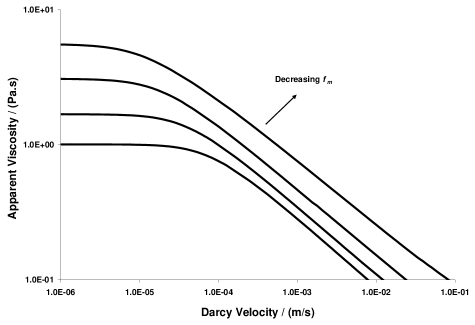
Figure 7.3: The Tardy algorithm sand pack results for $G_{o}$=0.1 Pa, $\mu_{\infty}$=0.001 Pa.s, $\mu_{o}$=1.0 Pa.s, $\lambda$=1.0 s, $k$=10^-5 Pa^-1, $f_{e}$=1.0, $m$=10 slices, with varying $f_{m}$ (1.0, 0.8, 0.6 and 0.4).

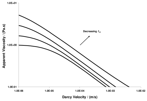
Figure 7.4: The Tardy algorithm Berea results for $G_{o}$=0.1 Pa, $\mu_{\infty}$=0.001 Pa.s, $\mu_{o}$=1.0 Pa.s, $\lambda$=1.0 s, $k$=10^-5 Pa^-1, $f_{e}$=1.0, $m$=10 slices, with varying $f_{m}$ (1.0, 0.8, 0.6 and 0.4).

7.3.2.2 Diverging-Converging

The investigation of the effect of diverging-converging geometry by expanding the radius of the capillaries at the middle revealed a thinning effect relative to the straight and converging-diverging geometries, as seen in Figures (7.5) and (7.6) for the sand pack and Berea networks respectively on a log-log scale. This is due to the increase in the conductance of the capillaries by enlarging the radius at the middle.

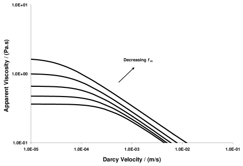
Figure 7.5: The Tardy algorithm sand pack results for $G_{o}$=0.1 Pa, $\mu_{\infty}$=0.001 Pa.s, $\mu_{o}$=1.0 Pa.s, $\lambda$=1.0 s, $k$=10^-5 Pa^-1, $f_{e}$=1.0, $m$=10 slices, with varying $f_{m}$ (0.8, 1.0, 1.2, 1.4 and 1.6).

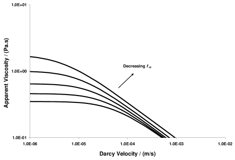
Figure 7.6: The Tardy algorithm Berea results for $G_{o}$=0.1 Pa, $\mu_{\infty}$=0.001 Pa.s, $\mu_{o}$=1.0 Pa.s, $\lambda$=1.0 s, $k$=10^-5 Pa^-1, $f_{e}$=1.0, $m$=10 slices, with varying $f_{m}$ (0.8, 1.0, 1.2, 1.4 and 1.6).

7.3.2.3 Number of Slices

As the number of slices of the capillaries increases, the algorithm converges to a stable and constant solution within acceptable numerical errors. This indicates that the numerical aspects of the algorithm are functioning correctly because the effect of discretization errors is expected to diminish by increasing the number of slices and hence decreasing their width. A sample graph of apparent viscosity versus number of slices for a typical data point is presented in Figure (7.7) for the sand pack and in Figure (7.8) for Berea.

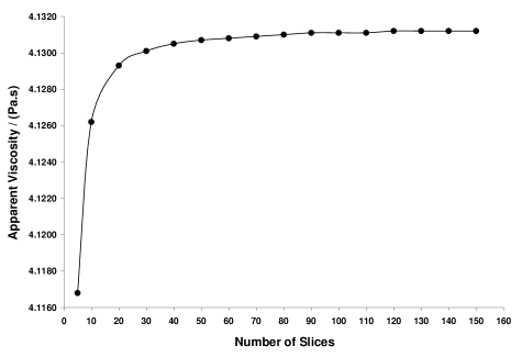
Figure 7.7: The Tardy algorithm sand pack results for $G_{o}$=1.0 Pa, $\mu_{\infty}$=0.001 Pa.s, $\mu_{o}$=1.0 Pa.s, $\lambda$=1.0 s, $k$=10^-5 Pa^-1, $f_{e}$=1.0, $f_{m}$=0.5, with varying number of slices for a typical data point ($\Delta P$=100 Pa).

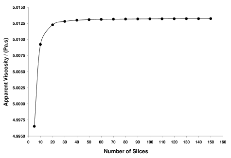
Figure 7.8: The Tardy algorithm Berea results for $G_{o}$=1.0 Pa, $\mu_{\infty}$=0.001 Pa.s, $\mu_{o}$=1.0 Pa.s, $\lambda$=1.0 s, $k$=10^-5 Pa^-1, $f_{e}$=1.0, $f_{m}$=0.5, with varying number of slices for a typical data point ($\Delta P$=200 Pa).

7.3.2.4 Boger Fluid

A Boger fluid behavior was observed when setting $\mu_{o}=\mu_{\infty}$. However, the apparent viscosity increased as the converging-diverging feature is intensified. This feature is demonstrated in Figure (7.9) for the sand pack and in Figure (7.10) for Berea on a log-log scale. Since Boger fluid is a limiting and obvious case, this behavior indicates that the model, as implemented, is well-behaved. The viscosity increase is a natural viscoelastic response to the radius tightening at the middle, as discussed earlier.

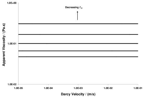
Figure 7.9: The Tardy algorithm sand pack results for $G_{o}$=1.0 Pa, $\mu_{\infty}$=$\mu_{o}$=0.1 Pa.s, $\lambda$=1.0 s, $k$=10^-5 Pa^-1, $f_{e}$=1.0, $m$=10 slices, with varying $f_{m}$ (0.6, 0.8, 1.0, 1.2 and 1.4).

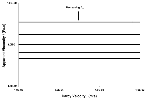
Figure 7.10: The Tardy algorithm Berea results for $G_{o}$=1.0 Pa, $\mu_{\infty}$=$\mu_{o}$=0.1 Pa.s, $\lambda$=1.0 s, $k$=10^-5 Pa^-1, $f_{e}$=1.0, $m$=10 slices, with varying $f_{m}$ (0.6, 0.8, 1.0, 1.2 and 1.4).

7.3.2.5 Elastic Modulus

The effect of the elastic modulus $G_{o}$ was investigated for shear-thinning fluids, i.e. $\mu_{o}>\mu_{\infty}$, by varying this parameter over several orders of magnitude while holding the others constant. It was observed that by increasing $G_{o}$, the high-shear apparent viscosities were increased while the low-shear viscosities remained constant and have not been affected. However, the increase at high-shear rates has almost reached a saturation point where beyond some limit the apparent viscosities converged to certain values despite a large increase in $G_{o}$. A sample of the results for this investigation is presented in Figure (7.11) for the sand pack and in Figure (7.12) for Berea on a log-log scale. The stability at low-shear rates is to be expected because at low flow rate regimes near the lower Newtonian plateau the non-Newtonian effects due to elastic modulus are negligible. As the elastic modulus increases, an increase in apparent viscosity due to elastic effects contributed by elastic modulus occurs. Eventually, a saturation will be reached when the contribution of this factor is controlled by other dominant factors and mechanisms from the porous medium and flow regime.

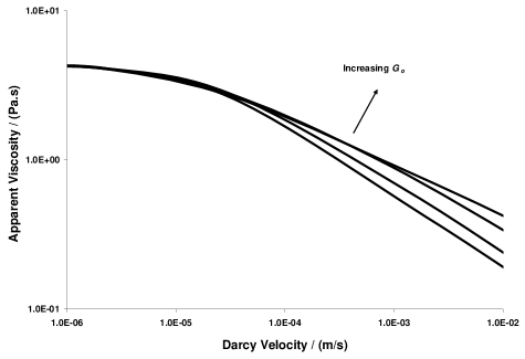
Figure 7.11: The Tardy algorithm sand pack results for $\mu_{\infty}$=0.001 Pa.s, $\mu_{o}$=1.0 Pa.s, $\lambda$=1.0 s, $k$=10^-5 Pa^-1, $f_{e}$=1.0, $f_{m}$=0.5, $m$=10 slices, with varying $G_{o}$ (0.1, 1.0, 10 and 100 Pa).

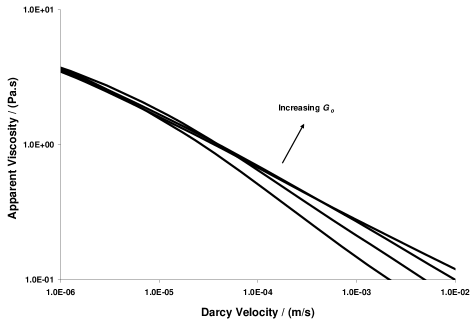
Figure 7.12: The Tardy algorithm Berea results for $\mu_{\infty}$=0.001 Pa.s, $\mu_{o}$=1.0 Pa.s, $\lambda$=1.0 s, $k$=10^-5 Pa^-1, $f_{e}$=1.0, $f_{m}$=0.5, $m$=10 slices, with varying $G_{o}$ (0.1, 1.0, 10 and 100 Pa).

7.3.2.6 Shear-Thickening

A slight shear-thickening effect was observed when setting $\mu_{o}<\mu_{\infty}$ while holding the other parameters constant. The effect of increasing $G_{o}$ on the apparent viscosities at high-shear rates was similar to the effect observed for the shear-thinning fluids though it was at a smaller scale. However, the low-shear viscosities are not affected, as in the case of shear-thinning fluids. A convergence for the apparent viscosities at high-shear rates for large values of $G_{o}$ was also observed as for shear-thinning. A sample of the results obtained in this investigation is presented in Figures (7.13) and (7.14) for the sand pack and Berea networks respectively on a log-log scale. It should be remarked that as the Bautista-Manero is originally a shear-thinning model, it should not be expected to fully-predict shear-thickening phenomenon. However, the observed behavior is a good sign for our model because as we push the algorithm beyond its limit, the results are still qualitatively reasonable.

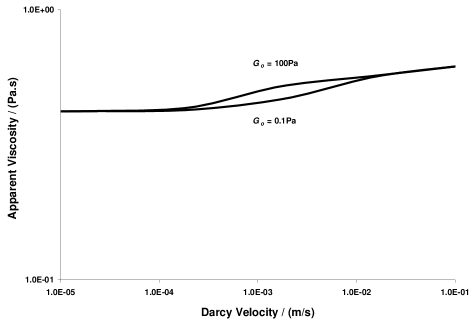
Figure 7.13: The Tardy algorithm sand pack results for $\mu_{\infty}$=10.0 Pa.s, $\mu_{o}$=0.1 Pa.s, $\lambda$=1.0 s, $k$=10^-4 Pa^-1, $f_{e}$=1.0, $f_{m}$=0.5, $m$=10 slices, with varying $G_{o}$ (0.1 and 100 Pa).

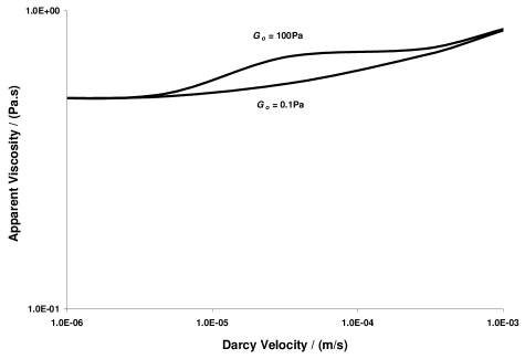
Figure 7.14: The Tardy algorithm Berea results for $\mu_{\infty}$=10.0 Pa.s, $\mu_{o}$=0.1 Pa.s, $\lambda$=1.0 s, $k$=10^-4 Pa^-1, $f_{e}$=1.0, $f_{m}$=0.5, $m$=10 slices, with varying $G_{o}$ (0.1 and 100 Pa).

7.3.2.7 Relaxation Time

The effect of the structural relaxation time $\lambda$ was investigated for shear-thinning fluids by varying this parameter over several orders of magnitude while holding the others constant. It was observed that by increasing the structural relaxation time, the apparent viscosities were steadily decreased. However, the decrease at high-shear rates has almost reached a saturation point where beyond some limit the apparent viscosities converged to certain values despite a large increase in $\lambda$. A sample of the results is given in Figure (7.15) for the sand pack and Figure (7.16) for Berea on a log-log scale. As we discussed earlier in this chapter, the effects of relaxation time are expected to ease as the relaxation time increases beyond a limit such that the effect of interaction with capillary constriction is negligible. Despite the fact that this feature requires extensive investigation for quantitative confirmation, the observed behavior seems qualitatively reasonable considering the flow regimes and the size of relaxation times of the sample results.

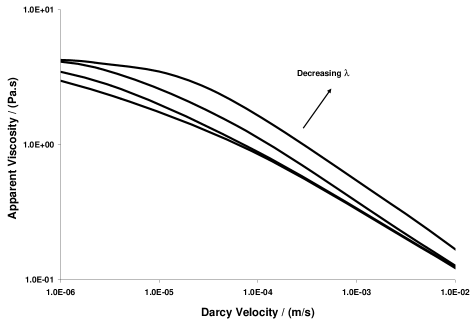
Figure 7.15: The Tardy algorithm sand pack results for $G_{o}$=1.0 Pa, $\mu_{\infty}$=0.001 Pa.s, $\mu_{o}$=1.0 Pa.s, $k$=10^-5 Pa^-1, $f_{e}$=1.0, $f_{m}$=0.5, $m$=10 slices, with varying $\lambda$ (0.1, 1.0, 10, and 100 s).

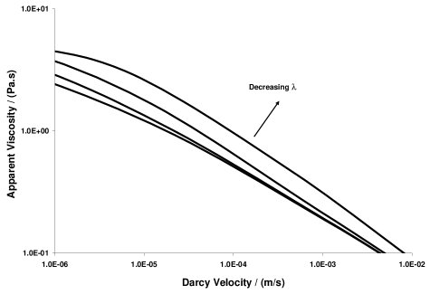
Figure 7.16: The Tardy algorithm Berea results for $G_{o}$=1.0 Pa, $\mu_{\infty}$=0.001 Pa.s, $\mu_{o}$=1.0 Pa.s, $k$=10^-5 Pa^-1, $f_{e}$=1.0, $f_{m}$=0.5, $m$=10 slices, with varying $\lambda$ (0.1, 1.0, 10, and 100 s).

7.3.2.8 Kinetic Parameter

The effect of the kinetic parameter for structure break down $k$ was investigated for shear-thinning fluids by varying this parameter over several orders of magnitude while holding the others constant. It was observed that by increasing the kinetic parameter, the apparent viscosities were generally decreased. However, in some cases the low-shear viscosities has not been substantially affected. A sample of the results is given in Figures (7.17) and (7.18) for the sand pack and Berea networks respectively on a log-log scale. The decrease in apparent viscosity on increasing the kinetic parameter is a natural response as the parameter quantifies structure break down and hence reflects thinning mechanisms. It is a general trend that the low flow rate regimes near the lower Newtonian plateau are usually less influenced by non-Newtonian effects. It will therefore come as no surprise that in some cases the low-shear viscosities experienced minor changes.

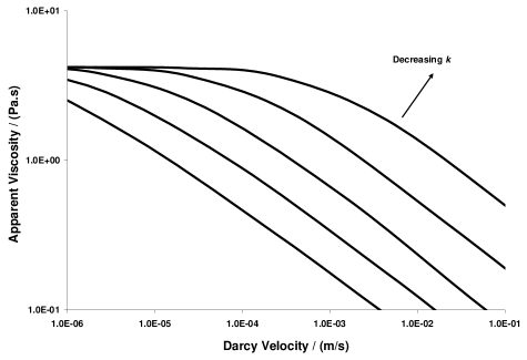
Figure 7.17: The Tardy algorithm sand pack results for $G_{o}$=1.0 Pa, $\mu_{\infty}$=0.001 Pa.s, $\mu_{o}$=1.0 Pa.s, $\lambda$=10 s, $f_{e}$=1.0, $f_{m}$=0.5, $m$=10 slices, with varying $k$ ($10^{-3}$, $10^{-4}$, $10^{-5}$, $10^{-6}$ and $10^{-7}$ Pa^-1).

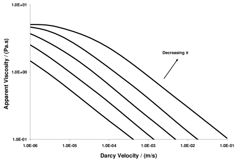
Figure 7.18: The Tardy algorithm Berea results for $G_{o}$=1.0 Pa, $\mu_{\infty}$=0.001 Pa.s, $\mu_{o}$=1.0 Pa.s, $\lambda$=1.0 s, $f_{e}$=1.0, $f_{m}$=0.5, $m$=10 slices, with varying $k$ ($10^{-3}$, $10^{-4}$, $10^{-5}$, $10^{-6}$ and $10^{-7}$ Pa^-1).

Chapter 8 Thixotropy and Rheopexy

Time-dependent fluids are defined to be those fluids whose viscosity depends on the duration of flow under isothermal conditions. For these fluids, a time-independent steady-state viscosity is eventually reached in steady flow situation. The time effect is often reversible though it may be partial. As a consequence, the trend of the viscosity change is overturned in time when the stress is reduced. The phenomenon is generally attributed to time-dependent thixotropic breakdown or rheopectic buildup of some particulate structure under relatively high stress followed by structural change in the opposite direction for lower stress, though the exact mechanism may not be certain. Furthermore, thixotropic buildup and rheopectic breakdown may also be a possibility [11, 7, 117, 118, 29].

Time-dependent fluids are generally divided into two main categories: thixotropic (work softening) whose viscosity gradually decreases with time at a constant shear rate, and rheopectic (work hardening or anti-thixotropy or negative thixotropy) whose viscosity increases under similar circumstances without an overshoot which is a characteristic feature of viscoelasticity. However, it has been proposed that rheopexy and negative thixotropy are different, and hence three categories of time-dependent fluids do exist [3, 11, 69]. It should be emphasized that in this thesis we may rely on the context and use “thixotropy” conveniently to indicate non-elastic time-dependence in general where the meaning is obvious.

Thixotropic fluids may be described as shear-thinning while the rheopectic as shear-thickening, in the sense that these effects take place on shearing, though they are effects of time-dependence. However, it has been suggested that thixotropy invariably occurs in circumstances where the liquid is shear-thinning (in the sense that viscosity levels decrease with increasing shear rate, other things being equal) and the anti-thixotropy is usually associated with shear-thickening. This may be behind the occasional confusion between thixotropy and shear-thinning [29, 26, 5, 119].

A substantial number of complex fluids display time-dependence phenomena, with thixotropy being more commonplace and better understood than rheopexy. Various mathematical models have been proposed to describe time-dependence behavior. These models include microstructural, continuum mechanics, and structural kinetics models [119, 118].

Thixotropic and rheopectic behaviors may be detected by the hysteresis loop test, as well as by the more direct steady shear test. In the loop test the substance is sheared cyclically and a graph of stress versus shear rate is obtained. A time-dependent fluid should display a hysteresis loop the area of which is a measure of the degree of thixotropy or rheopexy and may be used to quantify time-dependent behavior [7, 2, 69].

In theory, time-dependence effects can arise from thixotropic structural change or from time-dependent viscoelasticity or from both effects simultaneously. The existence of these two different types of time-dependent rheological behavior is generally recognized. Although it is convenient to distinguish between these as separate types of phenomena, real fluids can exhibit both types of rheological behavior simultaneously. Several physical distinctions between viscoelastic and thixotropic time-dependence have been made. The important one is that while the time-dependence of viscoelastic fluids arises because the response of stresses and strains in the fluid to changes in imposed strains and stresses respectively is not instantaneous, in thixotropic fluids such response is instantaneous and the time-dependent behavior arises purely because of changes in the structure of the fluid as a consequence of strain. Despite the fact that the mathematical theory of viscoelasticity has been developed to an advanced level, especially on the continuum mechanical front, relatively little work has been done on thixotropy and rheopexy. One reason is the lack of a comprehensive framework to describe the dynamics of thixotropy. This may partly explain why thixotropy is rarely incorporated in the constitutive equation when modeling the flow of non-Newtonian fluids. The underlying assumption is that in these situations the thixotropic effects have a negligible impact on the resulting flow field, and this allows great mathematical simplifications [120, 69, 117, 70, 71, 121].

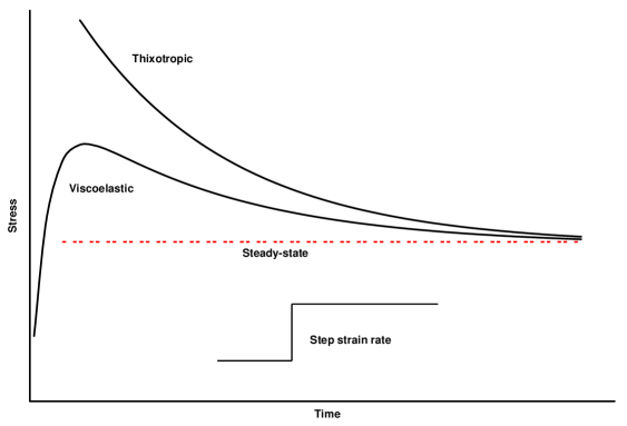
Figure 8.1: Comparison between time dependency in thixotropic and viscoelastic fluids following a step increase in strain rate.

Several behavioral distinctions can be made to differentiate between viscoelasticity and thixotropy. These include the presence or absence of some characteristic elastic features such as recoil and normal stresses. However, these signs may be of limited use in some practical situations involving complex fluids where these two phenomena coexist. In Figure (8.1) the behavior of these two types of fluids in response to step change in strain rate is compared. Although both fluids show signs of dependency on the past history, the graph suggests that inelastic thixotropic fluids do not possess a memory in the same sense as viscoelastic materials. The behavioral difference, such as the absence of elastic effects or the difference in the characteristic time scale associated with these phenomena, confirms this suggestion [29, 11, 120, 119].

Thixotropy, like viscoelasticity, is a phenomenon which can appear in a large number of systems. The time scale for thixotropic changes is measurable in various materials including important commercial and biological products. However, the investigation of thixotropy has been hampered by several difficulties. Consequently, the suggested thixotropic models seem unable to present successful quantitative description of thixotropic behavior especially for the transient state. In fact, even the most characteristic property of thixotropic fluids, i.e. the decay of viscosity or stress under steady shear conditions, presents difficulties in modeling and characterization [119, 120, 28].

The lack of a comprehensive theoretical framework to describe thixotropy is matched by a severe shortage on the experimental side. One reason is the difficulties confronted in measuring thixotropic systems with sufficient accuracy. The result is that very few systematic data sets can be found in the literature and this deficit hinders the progress in this field. Moreover, the characterization of the data in the absence of an agreed-upon mathematical structure may be questionable [117, 118].

8.1 Simulating Time-Dependent Flow in Porous Media

There are three major cases of simulating the flow of time-dependent fluids in porous media:

• The flow of strongly strain-dependent fluid in a porous medium which is not very homogeneous. This is very difficult to model because it is difficult to track the fluid elements in the pores and throats and determine their deformation history. Moreover, the viscosity function may not be well defined due to the mixing of fluid elements with various deformation history in the individual pores and throats.

• The flow of strain-independent or weakly strain-dependent fluid through porous media in general. A possible strategy is to apply single time-dependent viscosity function to all pores and throats at each instant of time and hence simulating time development as a sequence of Newtonian states.

• The flow of strongly strain-dependent fluid in a very homogeneous porous medium such that the fluid is subject to the same deformation in all network elements. The strategy for modeling this flow is to define an effective pore strain rate. Then using a very small time step the strain rate in the next instant of time can be found assuming constant strain rate. As the change in the strain rate is now known, a correction to the viscosity due to strain-dependency can be introduced.

  There are two possible problems in this strategy. The first is edge effects in the case of injection from a reservoir since the deformation history of the fluid elements at the inlet is different from the deformation history of the fluid elements inside the network. The second is that considerable computing resources may be required if very small time steps are used.

In the current work, thixotropic behavior is modeled within the Tardy algorithm as the Bautista-Manero fluid incorporates thixotropic as well as viscoelastic effects.

Chapter 9 Conclusions and Future Work

9.1 Conclusions

Here, we present some general results and conclusions that can be drawn from this work

• The network model has been extended to account for different types of non-Newtonian rheology: Ellis and Herschel-Bulkley models for time-independent, and Bautista-Manero for viscoelastic. The basis of the implementation in the first case is an analytical expression for the nonlinear relationship between flow rate and pressure drop in a single cylindrical element. These expressions are used in conjunction with an iterative technique to find the total flow across the network. For the Bautista-Manero viscoelastic model, the basis is a numerical algorithm originally suggested by Tardy. A modified version of this algorithm was used to investigate the effect of converging-diverging geometry on the steady-state viscoelastic flow.

• The general trends in behavior for shear-independent, shear-thinning and shear-thickening fluids with and without yield-stress for the time-independent category have been examined. Compared to an equivalent uniform bundle of tubes model, our networks yield at lower pressure gradients. Moreover, some elements remain blocked even at very high pressure gradients. The results also reveal that shear-thinning accentuates the heterogeneity of the network, while shear-thickening makes the flow more uniform.

• A comparison between the sand pack and Berea networks and a cubic network matching their characteristics has been made and some useful conclusions have been drawn.

• The network model successfully predicted several experimental data sets in the literature on Ellis fluids. Less satisfactory results were obtained for the Herschel-Bulkley fluids.

• The predictions were less satisfactory for yield-stress fluids of Herschel-Bulkley model. The reason is the inadequate representation of the pore space structure with regard to the yield process, that is the yield in a network depends on the actual shape of the void space rather than the flow conductance of the pores and throats. Other possible reasons for this failure are experimental errors and the occurrence of other physical effects which are not accounted for in our model, such as precipitation and adsorption.

• Several numerical algorithms related to yield-stress have been implemented in our non-Newtonian code and a comparison has been made between the two algorithms whose objective is to predict the threshold yield pressure of a network. These algorithms include the Invasion Percolation with Memory (IPM) of Kharabaf and the Path of Minimum Pressure (PMP) which is a novel and computationally more efficient technique than the IPM. The two methods gave similar predictions for the random networks and identical predictions for the cubic networks. An explanation was given for the difference observed in some cases of random networks as the algorithms are implemented with different assumptions on the possibility of flow backtracking.

• A comparison was also made between the IPM and PMP algorithms on one hand and the network flow simulation results on the other. An explanation was given for why these algorithms predict lower threshold yield pressure than the network simulation results.

• The implementation of the Bautista-Manero model in the form of a modified Tardy algorithm for steady-state viscoelastic flow has been examined and assessed. The generic behavior indicates qualitatively correct trends. A conclusion was reached that the current implementation is a proper basis for investigating the steady-state viscoelastic effects, and possibly some thixotropic effects, due to converging-diverging geometries in porous media. This implementation can also be used as a suitable base for further future development.

9.2 Recommendations for Future Work

Our recommendations for the future work are

• Extending the current non-Newtonian model to account for other physical phenomena such as adsorption and wall exclusion.

• Implementing other time-independent fluid models.

• Implementing two-phase flow of two non-Newtonian fluids.

• Considering more complex void space description either by using more elaborate networks or by superimposing more elaborate details on the current networks.

• Extending the analysis of the yield-stress fluids and investigating the effect of the actual shape of the void space on the yield point instead of relating the yield to the conductance of cylindrically-shaped capillaries.

• Examining the effect of converging-diverging geometry on the yield-stress of the network. The current implementation of the converging-diverging capillaries in the Tardy viscoelastic algorithm will facilitate this task.

• Elaborating the modified Tardy algorithm and thoroughly investigating its viscoelastic and thixotropic predictions in quantitative terms.

• Developing and implementing other transient and steady-state viscoelastic algorithms.

• Developing and implementing time-dependent algorithms in the form of pure thixotropic and rheopectic models such as the Stretched Exponential Model, though thixotropic effects are integrated within the Bautista-Manero fluid which is already implemented in the Tardy algorithm.

Appendix A

The Flow Rate of an Ellis Fluid in a Cylindrical Tube

Here, we derive an analytical expression for the volumetric flow rate in a cylindrical duct, with inner radius $R$ and length $L$, assuming Ellis flow. We apply the well-known general result, sometimes called the Weissenberg-Rabinowitsch equation or Rabinowitsch-Mooney equation [6, 12] which relates the flow rate $Q$ and the shear stress at the tube wall $\tau_{w}$ for laminar flow of time-independent fluids in a cylindrical tube. This equation, which can be derived considering the volumetric flow rate through the differential annulus between $r$ and $r+dr$ as shown in Figure (A.1), is given by [1, 6, 11]

$$\frac{Q}{\pi R^{3}}=\frac{1}{\tau^{3}_{w}}\int_{0}^{\tau_{w}}\tau^{2}\dot{\gamma}\ \mathrm{d}\tau$$ (A.1)

The derivation is based on the definition of the viscosity as the stress over strain rate. For Ellis fluid, the viscosity is given by [9, 10, 6, 11]

$$\mu=\frac{\mu_{o}}{1+\left(\frac{\tau}{\tau_{{}_{1/2}}}\right)^{\alpha-1}}$$ (A.2)

where $\mu_{o}$ is the low-shear viscosity, $\tau$ is the shear stress, $\tau_{{}_{1/2}}$ is the shear stress at which $\mu=\mu_{o}/2$ and $\alpha$ is an indicial parameter in the Ellis model.

From this expression we obtain a formula for the shear rate

$$\dot{\gamma}=\frac{\tau}{\mu}=\frac{\tau}{\mu_{o}}\left[1+\left(\frac{\tau}{\tau_{{}_{1/2}}}\right)^{\alpha-1}\right]$$ (A.3)

On substituting this into Equation (A.1), integrating and simplifying we obtain

$$Q = \frac{\pi R^{3}\tau_{w}}{4\mu_{o}}\left[1+\frac{4}{\alpha+3}\left(\frac{\tau_{w}}{\tau_{{}_{1/2}}}\right)^{\alpha-1}\right]$$ (A.4)

$$= \frac{\pi R^{4}\Delta P}{8L\mu_{o}}\left[1+\frac{4}{\alpha+3}\left(\frac{R\Delta P}{2L\tau_{{}_{1/2}}}\right)^{\alpha-1}\right]$$

where $\tau_{w}=\Delta PR/2L$ and $\Delta P$ is the pressure drop across the tube.

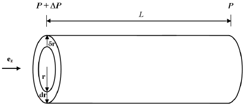
Figure A.1: Schematic diagram of a cylindrical annulus used to derive analytical expressions for the volumetric flow rate of Ellis and Herschel-Bulkley fluids.

Appendix B

The Flow Rate of a Herschel-Bulkley Fluid in a Cylindrical Tube

Here, we present two methods for deriving an analytical expression for the volumetric flow rate in a cylindrical duct, with inner radius $R$ and length $L$, assuming Herschel-Bulkley flow.

B.1 First Method

In this method, Equation (A.1) is used [1] as in the case of Ellis fluid. For a Herschel-Bulkley fluid

$$\dot{\gamma}=\left(\frac{\tau}{C}-\frac{\tau_{o}}{C}\right)^{\frac{1}{n}}$$ (B.1)

On substituting (B.1) into (A.1), integrating and simplifying we obtain

$$Q=\frac{8\pi}{C^{\frac{1}{n}}}\left(\frac{L}{\Delta P}\right)^{3}\left(\tau_{w}-\tau_{o}\right)^{1+\frac{1}{n}}\left[\frac{\left(\tau_{w}-\tau_{o}\right)^{2}}{3+1/n}+\frac{2\tau_{o}\left(\tau_{w}-\tau_{o}\right)}{2+1/n}+\frac{\tau_{o}^{2}}{1+1/n}\right]$$ (B.2)

B.2 Second Method

In this method we use cylindrical polar coordinate system where the tube axis coincides with the coordinate $z$-axis and the flow is in the positive $z$-direction. Newton’s second law [$m$a = $\sum_{i}$F_i] is applied to a cylindrical annulus of fluid with inner radius $r$, outer radius $r$+d$r$ and length $L$, as illustrated in Figure (A.1). Assuming negligible body forces, we have two surface forces; one is due to the pressure gradient and the other is due to the shear stress, that is

$$(2\pi r\delta rL\rho\mathrm{a}){\bf{e}}_{z}\cong(2\pi r\delta r\Delta P){\bf{e}}_{z}-[2\pi(r+\delta r)(\tau+\delta\tau)L-2\pi r\tau L]{\bf{e}}_{z}$$ (B.3)

Dividing by $2\pi\delta rL$, simplifying and taking the scalar form, we obtain

$$\rho\mathrm{a}\cong\frac{\Delta P}{L}-(\frac{\tau}{r}+\frac{\delta\tau}{\delta r}+\frac{\delta\tau}{r})$$ (B.4)

Taking the limit when $\delta r\rightarrow 0$, and hence $\delta\tau\rightarrow 0$, we obtain the exact relation

$$\rho\mathrm{a}=\frac{\Delta P}{L}-(\frac{\tau}{r}+\frac{\mathrm{d}\tau}{\mathrm{d}r})$$ (B.5)

For steady flow, a [$=\frac{\mathrm{d}u_{z}}{\mathrm{d}t}$] is zero, thus

$$\frac{\mathrm{d}\tau}{\mathrm{d}r}+\frac{\tau}{r}=\frac{\Delta P}{L}$$ (B.6)

On integrating this relation we obtain

$$\tau=\frac{\Delta Pr}{2L}+\frac{A}{r}$$ (B.7)

where $A$ is the constant of integration.

At $r=0$, $\tau$ is finite, so $A=0$. From this we obtain

$$\tau=\frac{\Delta Pr}{2L}$$ (B.8)

From the definition of the shear rate, $\dot{\gamma}=\frac{\mathrm{d}u_{z}}{\mathrm{d}r}$, we obtain

$$u_{z}=\int\dot{\gamma}\mathrm{d}r$$ (B.9)

For Herschel-Bulkley fluid

$$\dot{\gamma}=\left(\frac{\tau}{C}-\frac{\tau_{o}}{C}\right)^{\frac{1}{n}}$$ (B.10)

Substituting for $\tau$ from (B.8) into (B.10) we obtain

$$\dot{\gamma}=\left(\frac{\Delta P}{2LC}r-\frac{\tau_{o}}{C}\right)^{\frac{1}{n}}$$ (B.11)

Inserting (B.11) into (B.9), integrating and applying the second boundary condition, i.e $u_{z}(r$=$R)=0$, we obtain

$$u_{z}(r)=\frac{n}{1+n}\left(\frac{2LC}{\Delta P}\right)\left[\left(\frac{\Delta P}{2LC}R-\frac{\tau_{o}}{C}\right)^{1+\frac{1}{n}}-\left(\frac{\Delta P}{2LC}r-\frac{\tau_{o}}{C}\right)^{1+\frac{1}{n}}\right]$$ (B.12)

In fact, Equation (B.9) is valid only for $\dot{\gamma}>0$, and this condition requires that at any point with finite shear rate, $\tau>\tau_{o}$, as can be seen from (B.10). Equation (B.8) then implies that the region with $r\leq r_{o}=\frac{2L\tau_{o}}{\Delta P}$ is a shear-free zone. From the continuity of the velocity field, we conclude that

$$u_{z}(0\leq r\leq r_{o})=\frac{n}{1+n}\left(\frac{2LC}{\Delta P}\right)\left(\frac{\Delta P}{2LC}R-\frac{\tau_{o}}{C}\right)^{1+\frac{1}{n}}$$ (B.13)

The volumetric flow rate is given by

$$Q=\int_{0}^{R}2\pi ru_{z}\mathrm{d}r$$ (B.14)

that is

$$Q=\int_{0}^{r_{o}}2\pi ru_{z}(0\leq r\leq r_{o})\mathrm{d}r+\int_{r_{o}}^{R}2\pi ru_{z}(r>r_{o})\mathrm{d}r$$ (B.15)

On inserting (B.13) into the first term of (B.15) and (B.12) into the second term of (B.15), integrating and simplifying we obtain

$$Q=\frac{8\pi}{C^{\frac{1}{n}}}\left(\frac{L}{\Delta P}\right)^{3}\frac{\left(\tau_{w}-\tau_{o}\right)^{1+\frac{1}{n}}}{(1+1/n)}\left[\frac{2(\tau_{w}-\tau_{o})^{2}}{(3+1/n)(2+1/n)}+\frac{2\tau_{w}(\tau_{o}-\tau_{w})}{(2+1/n)}+\tau_{w}^{2}\right]$$ (B.16)

Although (B.2) and (B.16) look different, they are mathematically identical, as each one can be obtained from the other by algebraic manipulation.

There are three important special cases for Herschel-Bulkley fluid. These, with the volumetric flow rate expressions, are

1. Newtonian
   

   $$Q=\frac{\pi R^{4}\Delta P}{8LC}$$ (B.17)

2. Power-law 
   

   $$Q=\frac{\pi R^{4}\Delta P^{1/n}}{8LC^{1/n}}\left(\frac{4n}{3n+1}\right)\left(\frac{2L}{R}\right)^{1-1/n}$$ (B.18)

3. Bingham plastic
   

   $$Q=\frac{\pi R^{4}\Delta P}{8LC}\left[\frac{1}{3}\left(\frac{\tau_{o}}{\tau_{w}}\right)^{4}-\frac{4}{3}\left(\frac{\tau_{o}}{\tau_{w}}\right)+1\right]$$ (B.19)

Each one of these expressions can be derived directly by these two methods. Moreover, they can be obtained by substituting the relevant conditions in the flow rate expression for Herschel-Bulkley fluid. This serves as a consistency check.

Appendix C

Yield Condition for a Single Tube

The volumetric flow rate of a Herschel-Bulkley fluid in a cylindrical tube is given by Equation (B.2). For a fluid with yield-stress, the flow occurs iff $Q>0$. Assuming $\tau_{o}$, $R$, $L$, $C$, $\Delta P$, $n$ $>0$, it is straightforward to show that the condition $Q>0$ is satisfied iff   $\left(\tau_{w}-\tau_{o}\right)>0$, that is

$$\tau_{w}=\frac{\Delta PR}{2L}>\tau_{o}$$ (C.1)

Hence, the threshold pressure gradient, above which the flow starts, is

$$|\nabla P_{th}|={\frac{2\tau_{o}}{R}}$$ (C.2)

Alternatively, the flow occurs when the shear stress at wall exceeds the yield-stress, i.e.

$$\tau_{w}>\tau_{o}$$ (C.3)

which leads to the same condition. This second argument is less obvious but more general than the first.

Appendix D

The Radius of the Bundle of Tubes to Compare with the Networks

In Chapter (4) a comparison was made between two networks representing sand pack and Berea porous media and a bundle of capillaries of uniform radius model. The networks and the bundle are assumed to have the same porosity and Darcy velocity under Newtonian flow condition.

Here, we derive an expression for the radius of the tubes in the bundle. We equate Poiseuille for a single tube in the bundle divided by $d^{2}$, where $d$ is the side of the square enclosing the tube cross section in the bundle’s matrix, to the Darcy velocity for the network, that is

$$q=\frac{\pi R^{4}\Delta P}{8\mu Ld^{2}}=\frac{K\Delta P}{\mu L}$$ (D.1)

Thus

$$\frac{\pi R^{4}}{8d^{2}}=K$$ (D.2)

The porosity of a bundle of $N$ tubes is

$$\frac{NL\pi R^{2}}{NLd^{2}}=\frac{\pi R^{2}}{d^{2}}$$ (D.3)

On equating this to the network porosity, $\phi$, substituting into (D.2) and rearranging we obtain

$$R=\sqrt{\frac{8K}{\phi}}$$ (D.4)

Appendix E

Terminology of Flow and Viscoelasticity

A tensor is an array of numbers which transform according to certain rules under coordinate change. In a three-dimensional space, a tensor of order $n$ has $3^{n}$ components which may be specified with reference to a given coordinate system. Accordingly, a scalar is a zero-order tensor and a vector is a first-order tensor.

A stress is defined as a force per unit area. Because both force and area are vectors, considering the orientation of the normal to the area, stress has two directions associated with it instead of one as with vectors. This indicates that stress should be represented by a second-order tensor, given in Cartesian coordinate system by

$$\mbox{\boldmath{$\tau$}}=\left(\begin{array}[]{ccc}\tau_{xx}&\tau_{xy}&\tau_{xz}\\ \tau_{yx}&\tau_{yy}&\tau_{yz}\\ \tau_{zx}&\tau_{zy}&\tau_{zz}\\ \end{array}\right)$$ (E.1)

where $\tau_{ij}$ is the stress in the $j$-direction on a surface normal to the $i$-axis. A shear stress is a force that a flowing liquid exerts on a surface, per unit area of that surface, in the direction parallel to the flow. A normal stress is a force per unit area acting normal or perpendicular to a surface. The components with identical subscripts represent normal stresses while the others represent shear stresses. Thus $\tau_{xx}$ is a normal stress acting in the $x$-direction on a face normal to $x$-direction, while $\tau_{yx}$ is a shear stress acting in the $x$-direction on a surface normal to the $y$-direction, positive when material at greater $y$ exerts a shear in the positive $x$-direction on material at lesser $y$. Normal stresses are conventionally positive when tensile. The stress tensor is symmetric that is $\tau_{ij}=\tau_{ji}$ where $i$ and $j$ represent $x$, $y$ or $z$. This symmetry is required by angular momentum considerations to satisfy equilibrium of moments about the three axes of any fluid element. This means that the state of stress at a point is determined by six, rather than nine, independent stress components.

Viscoelastic fluids show normal stress differences in steady shear flows. The first normal stress difference $N_{1}$ is defined as

$$N_{1}=\tau_{11}-\tau_{22}$$ (E.2)

where $\tau_{11}$ is the normal stress component acting in the direction of flow and $\tau_{22}$ is the normal stress in the gradient direction. The second normal stress difference $N_{2}$ is defined as

$$N_{2}=\tau_{22}-\tau_{33}$$ (E.3)

where $\tau_{33}$ is the normal stress component in the indifferent direction. The magnitude of $N_{2}$ is in general much smaller than $N_{1}$. For some viscoelastic fluids, $N_{2}$ may be virtually zero. Often not the first normal stress difference $N_{1}$ is given, but a related quantity: the first normal stress coefficient. This coefficient is defined by $\Psi_{1}=\frac{N_{1}}{\dot{\gamma}^{2}}$ and decreases with increasing shear rate. Different conventions about the sign of the normal stress differences do exist. However, in general $N_{1}$ and $N_{2}$ show opposite signs. Viscoelastic solutions with almost the same viscosities may have very different values of normal stress differences. The presence of normal stress differences is a strong indication of viscoelasticity, though some associate these properties with non-viscoelastic fluids.

The total stress tensor, also called Cauchy stress tensor, is usually divided into two parts: hydrostatic stress tensor and extra stress tensor. The former represents the hydrostatic pressure while the latter represents the shear and extensional stresses caused by the flow. In equilibrium the pressure reduces to the hydrostatic pressure and the extra stress tensor $\tau$ vanishes. The extra stress tensor is determined by the deformation history and has to be specified by the constitutive equation of the particular fluid.

The rate-of-strain or rate-of-deformation tensor is a symmetric second-order tensor which gives the components, both extensional and shear, of the strain rate. In Cartesian coordinate system it is given by:

$$\mbox{\boldmath{$\dot{\gamma}$}}=\left(\begin{array}[]{ccc}\dot{\gamma}_{xx}&\dot{\gamma}_{xy}&\dot{\gamma}_{xz}\\ \dot{\gamma}_{yx}&\dot{\gamma}_{yy}&\dot{\gamma}_{yz}\\ \dot{\gamma}_{zx}&\dot{\gamma}_{zy}&\dot{\gamma}_{zz}\\ \end{array}\right)$$ (E.4)

where $\dot{\gamma}_{xx}$, $\dot{\gamma}_{yy}$ and $\dot{\gamma}_{zz}$ are the extensional components while the others are the shear components. These components are given by:

$$\dot{\gamma}_{xx}=2\frac{\partial v_{x}}{\partial x}\verb| |\dot{\gamma}_{yy}=2\frac{\partial v_{y}}{\partial y}\verb| |\dot{\gamma}_{zz}=2\frac{\partial v_{z}}{\partial z}\verb| |$$

$$\dot{\gamma}_{xy}=\dot{\gamma}_{yx}=\frac{\partial v_{x}}{\partial y}+\frac{\partial v_{y}}{\partial x}$$

$$\dot{\gamma}_{yz}=\dot{\gamma}_{zy}=\frac{\partial v_{y}}{\partial z}+\frac{\partial v_{z}}{\partial y}$$

$$\dot{\gamma}_{xz}=\dot{\gamma}_{zx}=\frac{\partial v_{x}}{\partial z}+\frac{\partial v_{z}}{\partial x}$$ (E.5)

where $v_{x}$, $v_{y}$ and $v_{z}$ are the velocity components in the respective directions $x$, $y$ and $z$.

The stress tensor is related to the rate-of-strain tensor by the constitutive or rheological equation of the fluid which takes a differential or integral form. The rate-of-strain tensor $\dot{\gamma}$ is related to the fluid velocity vector v, which describes the steepness of velocity variation as one moves from point to point in any direction in the flow at a given instant in time, by the relation

$$\mbox{\boldmath{$\dot{\gamma}$}}=\nabla\mbox{\bf{v}}+(\nabla\mbox{\bf{v}})^{\textrm{T}}$$ (E.6)

where $(.)^{\textrm{T}}$ is the tensor transpose and $\nabla\mbox{\bf{v}}$ is the fluid velocity gradient tensor defined by

$$\nabla\mbox{\bf{v}}=\left(\begin{array}[]{ccc}\frac{\partial v_{x}}{\partial x}&\frac{\partial v_{x}}{\partial y}&\frac{\partial v_{x}}{\partial z}\\ \frac{\partial v_{y}}{\partial x}&\frac{\partial v_{y}}{\partial y}&\frac{\partial v_{y}}{\partial z}\\ \frac{\partial v_{z}}{\partial x}&\frac{\partial v_{z}}{\partial y}&\frac{\partial v_{z}}{\partial z}\end{array}\right)$$ (E.7)

with $\mbox{\bf{v}}=(v_{x},v_{y},v_{z})$. It should be remarked that the sign and index conventions used in the definitions of these tensors are not universal.

A fluid possesses viscoelasticity if it is capable of storing elastic energy. A sign of this is that stresses within the fluid persist after the deformation has ceased. The duration of time over which appreciable stresses persist after cessation of deformation gives an estimate of what is called the relaxation time. The relaxation and retardation times, $\lambda_{1}$ and $\lambda_{2}$ respectively, are important physical properties of viscoelastic fluids because they characterize whether viscoelasticity is likely to be important within an experimental or observational timescale. They usually have the physical significance that if the motion is suddenly stopped the stress decays as $e^{-t/\lambda_{1}}$, and if the stress is removed the rate of strain decays as $e^{-t/\lambda_{2}}$.

For viscous flow, the Reynolds number $Re$ is a dimensionless number defined as the ratio of the inertial to viscous forces and is given by

$$Re=\frac{\rho l_{c}v_{c}}{\mu}$$ (E.8)

where $\rho$ is the mass density of the fluid, $l_{c}$ is a characteristic length of the flow system, $v_{c}$ is a characteristic speed of the flow and $\mu$ is the viscosity of the fluid.

For viscoelastic fluids the key dimensionless group is the Deborah number which is a measure of the elasticity of the fluid. This number may be interpreted as the ratio of the magnitude of the elastic forces to that of the viscous forces. It is defined as the ratio of a characteristic time of the fluid $\lambda_{c}$ to a characteristic time of the flow system $t_{c}$

$$De=\frac{\lambda_{c}}{t_{c}}$$ (E.9)

The Deborah number is zero for a Newtonian fluid and is infinite for a Hookean elastic solid. High Deborah numbers correspond to elastic behavior and low Deborah numbers to viscous behavior. As the characteristic times are process-dependent, materials may not have a single Deborah number associated with them.

Another dimensionless number which measures the elasticity of the fluid is the Weissenberg number $We$. It is defined as the product of a characteristic time of the fluid $\lambda_{c}$ and a characteristic strain rate $\dot{\gamma}_{c}$ in the flow

$$We=\lambda_{c}\dot{\gamma}_{c}$$ (E.10)

Other definitions to Deborah and Weissenberg numbers are also in common use and some even do not differentiate between the two numbers. The characteristic time of the fluid may be taken as the largest time constant describing the molecular motions, or a time constant in a constitutive equation. The characteristic time for the flow can be the time interval during which a typical fluid element experiences a significant sequence of kinematic events or it is taken to be the duration of an experiment or experimental observation. Many variations in defining and quantifying these characteristics do exit, and this makes Deborah and Weissenberg numbers not very well defined and measured properties and hence the interpretation of the experiments in this context may not be totally objective.

The Boger fluids are constant-viscosity purely elastic non-Newtonian fluids. They played important role in the recent development of the theory of fluid elasticity as they allow dissociation between elastic and viscous effects. Boger realized that the complication of variable viscosity effects can be avoided by employing test liquids which consist of low concentrations of flexible high molecular weight polymers in very viscous solvents, and these solutions are nowadays called Boger fluids.

Appendix F

Converging-Diverging Geometry and Tube Discretization

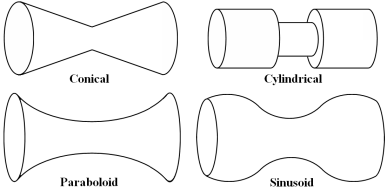
Figure F.1: Examples of corrugated capillaries which can be used to model converging-diverging geometry in porous media.

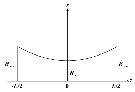
Figure F.2: Radius variation in the axial direction for a corrugated paraboloid capillary using a cylindrical coordinate system.

There are many simplified converging-diverging geometries for corrugated capillaries which can be used to model the flow of viscoelastic fluids in porous media; some suggestions are presented in Figure (F.1). In this study we adopted the paraboloid and hence developed simple formulae to find the radius as a function of the distance along the tube axis, assuming cylindrical coordinate system, as shown in Figure (F.2).

For the paraboloid depicted in Figure (F.2), we have

$$r(z)=az^{2}+bz+c$$ (F.1)

Since

$$r(-L/2)=r(L/2)=R_{max}\verb| |\&\verb| |r(0)=R_{min}$$ (F.2)

the paraboloid is uniquely identified by these three points. On substituting and solving these equations simultaneously, we obtain

$$a=\left(\frac{2}{L}\right)^{2}(R_{max}-R_{min})\verb| |b=0\verb| |\&\verb| |c=R_{min}$$ (F.3)

that is

$$r(z)=\left(\frac{2}{L}\right)^{2}(R_{max}-R_{min})z^{2}+R_{min}$$ (F.4)

In the modified Tardy algorithm for steady-state viscoelastic flow which we implemented in our non-Newtonian code, when a capillary is discretized into $m$ slices the radius $r(z)$ is sampled at $m$ $z$-points given by

$$z=-\frac{L}{2}+k\frac{L}{m}\verb| |(k=1,...,m)$$ (F.5)

More complex polynomial and sinusoidal converging-diverging profiles can also be modeled using this approach.

Appendix G

The Sand Pack and Berea Networks

The sand pack and Berea networks used in this study are those of Statoil (Øren and coworkers [83, 84]). They are constructed from voxel images generated by simulating the geological processes by which the porous medium was formed. The physical and statistical properties of the networks are presented in Tables (G.1) and (G.2).

The Berea network has more complex and less homogeneous structure than the sand pack. A sign of this is the bimodal nature of the Berea pore and throat size distributions. The details can be found in Lopez [80]. This fact may be disputed by the broader distributions of the sand pack indicated by broader ranges and larger standard deviations as seen in Tables (G.1) and (G.2). However, the reason for this is the larger averages of the sand pack properties. By normalizing the standard deviations to their corresponding averages, the sand pack will have narrower distributions for some of the most important features that control the flow and determine the physical properties of the network. These include the size distribution of inscribed radius of pores and throats. Furthermore, our judgement, which is shared by Lopez [80], is based on more thorough inspection to the behavior of the two networks in practical situations.

Despite the fact that the sand pack network seems to have some curious properties as it includes some eccentric elements such as super-connected pores and very long throats, we believe that these peculiarities have very little impact on the network behavior in general. The reason is that these elements are very few and their influence is diluted in a network of several thousands of normal pores and throats, especially for the fluids with no yield-stress. As for yield-stress fluids, the effect of these extreme elements may not be negligible if they occurr to aggregate in a favorable combination. However, it seems that this is not the case. A graphic demonstration of this fact is displayed in Figure (4.5) where the number of elements spanning the network (8 -10) when flow starts is comparable to the lattice size of the network (15$\times$15$\times$15). This rules out the possibility of a correlated streak of unusually large pores and throats. Our conviction is that 8 -10 moderately-large throats spanning a network of this size is entirely normal and do not involve eccentric elements. It is totally natural for yield-stress flow to start with the elements whose size is higher than the average.

It is noteworthy that the results of yield-free fluids are almost independent of the calculation box as long as the pertinent bulk properties are retained and provided that the width of the slice is sufficiently large to be representative of the network and mask the pore scale fluctuations. This is in sharp contrast with the yield-stress fluids where the results are highly dependent on the location of the calculation box as the yield-stress of a network is highly dependent on the nature of its elements and their topology and geometry. These observations are confirmed by a large number of simulation runs; and as for yield-stress fluids can be easily seen in Tables (6.1-6.4).

Table G.1: Physical and statistical properties of the sand pack network.

General
Size	2.5mm $\times$ 2.5mm $\times$ 2.5mm
Total number of elements	13490
Absolute permeability ($10^{-12}$m2)	93.18
Formation factor	2.58
Porosity	0.338
Clay bound porosity	0.00
No. of connections to inlet	195
No. of connections to outlet	158
Triangular shaped elements (%)	94.69
Square shaped elements (%)	1.56
Circular shaped elements (%)	3.75
Physically isolated elements (%)	0.00
Pores
Total number	3567
No. of triangular shaped	3497
No. of square shaped	70
No. of circular shaped	0
No. of physically isolated	0
	Min.	Max.	Ave.	St. Dev.
Connection number	1	99	5.465	4.117
Center to center length ($10^{-6}$m)	5.00	2066.62	197.46	176.24
Inscribed radius ($10^{-6}$m)	2.36	98.29	39.05	15.78
Shape factor	0.0146	0.0625	0.0363	0.0081
Volume ($10^{-15}$m3)	0.13	73757.26	1062.42	2798.79
Clay volume ($10^{-15}$m3)	0.00	0.00	0.00	0.00
Throats
Total number	9923
No. of triangular shaped	9277
No. of square shaped	140
No. of circular shaped	506
No. of physically isolated	0
	Min.	Max.	Ave.	St. Dev.
Length ($10^{-6}$m)	1.67	153.13	30.61	16.31
Inscribed radius ($10^{-6}$m)	0.50	85.57	23.71	11.19
Shape factor	0.0067	0.0795	0.0332	0.0137
Volume ($10^{-15}$m3)	0.13	2688.18	155.93	151.18
Clay volume ($10^{-15}$m3)	0.00	0.00	0.00	0.00

No. = Number Min. = Minimum Max. = Maximum Ave. = Average St. Dev. = Standard Deviation.

Note: The size-dependent properties, such as absolute permeability, are for the original network with no scaling. All data are for the complete network, i.e. for a calculation box with a lower boundary $x_{{}_{l}}=0.0$ and an upper boundary $x_{{}_{u}}=1.0$.

Table G.2: Physical and statistical properties of the Berea network.

General
Size	3.0mm $\times$ 3.0mm $\times$ 3.0mm
Total number of elements	38495
Absolute permeability ($10^{-12}$m2)	2.63
Formation factor	14.33
Porosity	0.183
Clay bound porosity	0.057
No. of connections to inlet	254
No. of connections to outlet	267
Triangular shaped elements (%)	92.26
Square shaped elements (%)	6.51
Circular shaped elements (%)	1.23
Physically isolated elements (%)	0.02
Pores
Total number	12349
No. of triangular shaped	11794
No. of square shaped	534
No. of circular shaped	21
No. of physically isolated	6
	Min.	Max.	Ave.	St. Dev.
Connection number	1	19	4.192	1.497
Center to center length ($10^{-6}$m)	4.28	401.78	115.89	48.81
Inscribed radius ($10^{-6}$m)	3.62	73.54	19.17	8.47
Shape factor	0.0113	0.0795	0.0332	0.0097
Volume ($10^{-15}$m3)	1.56	10953.60	300.55	498.53
Clay volume ($10^{-15}$m3)	0.00	8885.67	88.30	353.42
Throats
Total number	26146
No. of triangular shaped	23722
No. of square shaped	1972
No. of circular shaped	452
No. of physically isolated	3
	Min.	Max.	Ave.	St. Dev.
Length ($10^{-6}$m)	1.43	78.94	13.67	5.32
Inscribed radius ($10^{-6}$m)	0.90	56.85	10.97	7.03
Shape factor	0.0022	0.0795	0.0346	0.0139
Volume ($10^{-15}$m3)	0.49	766.42	48.07	43.27
Clay volume ($10^{-15}$m3)	0.00	761.35	17.66	34.89

No. = Number Min. = Minimum Max. = Maximum Ave. = Average St. Dev. = Standard Deviation.

Note: The size-dependent properties, such as absolute permeability, are for the original network with no scaling. All data are for the complete network, i.e. for a calculation box with a lower boundary $x_{{}_{l}}=0.0$ and an upper boundary $x_{{}_{u}}=1.0$.

Appendix H

The Manual of the Non-Newtonian Code

The computer code which is developed during this study is based on the non-Newtonian code by Xavier Lopez [80, 81]. The latter was constructed from an early version of the Newtonian code by Per Valvatne [78, 79]. The non-Newtonian code in its current state simulates single-phase flow only, as the code is tested and debugged for this case only. However, all features of the two-phase flow which are inherited from the parent code are left intact and can be easily activated for future development. Beside the Carreau model inherited from the original code of Lopez, the current code can simulate the flow of Ellis and Herschel-Bulkley fluids. Several algorithms related to yield-stress and a modified version of the Tardy algorithm to simulate steady-state viscoelastic flow using a Bautista-Manero model are also implemented. The code can be downloaded from this URL: http://www3.imperial.ac.uk/earthscienceandengineering/research/perm/
porescalemodelling/software.

The program uses a keyword based input file “0.inputFile.dat”. All keywords are optional with no order required. If keywords are omitted, default values will be used. Comments in the data file are indicated by “%”, resulting in the rest of the line being discarded. All data should be on a single line following the keyword (possibly separated by comment lines).

The general flowing sequence of the program is as follows:

• The program starts by reading the input and network data files followed by creating the network.

• For fluids with yield-stress, the program executes IPM (Invasion Percolation with Memory) and PMP (Path of Minimum Pressure) algorithms to predict the threshold yield pressure of the network. This is followed by an iterative simulation algorithm to find the network’s actual threshold yield pressure to the required number of decimal places.

• Single-phase flow with Newtonian fluid is simulated and the fluid-related network properties, such as absolute permeability, are obtained.

• Single-phase flow with Newtonian and non-Newtonian fluids is simulated over a pressure line.

In all stages, informative messages are issued about the program flow and the data obtained. The program also creates several output data files. These are:

1. The main output data file which contains the data in the input file and the screen output. This will be discussed under the “TITLE” keyword.

2. “01.FNProp” file which contains data on the network and fluid properties.

3. “1.Pressure” file which contains the pressure points.

4. “2.Gradient” file which contains the pressure gradients corresponding to the pressure points in the previous file.

5. “3.FlowRate” file which contains the corresponding volumetric flow rates for the single-phase non-Newtonian flow.

6. “4.DarcyVelocity” file which contains the corresponding Darcy velocities.

7. “5.Viscosity” file which contains the corresponding apparent viscosities.

8. “6.AvrRadFlow” file which contains the average radius of the flowing throats of the network at each pressure point. This is mainly useful in the case of a yield-stress fluid.

9. “7.PerCentFlow” file which contains the percentage of the flowing throats at each pressure point. This is mainly useful in the case of a yield-stress fluid.

The reason for keeping the data separated in different files is to facilitate flexible post-processing by spreadsheets or other programs. Two samples of spreadsheets used to process the data are included. The spreadsheets are designed to read the data files directly on launching the application. What the user needs is to “Enable automatic refresh” after redefining the path to the required data files using “Edit Text Import” option. The relevant cells to do this path redefinition are blue-colored.

It should be remarked that all the data in the files are valid data obtained from converged-to pressure points. If for some reason the program failed to converge at a pressure point, all the data related to that point will be ignored and not saved to the relevant files to keep the integrity of the data intact.

All physical data in the input file are in SI unit system.

——————————————————————
TITLE
The program generates a file named “title.prt” containing the date and time of simulation, the data in the input file and the screen output. Moreover, the user can also define the directory to which all the output files will be saved.

1. Title of the “.prt” file.

2. The directory to which all output files should be written.

If this keyword is omitted, the default is “0.Results ./”.

TITLE
% Title of .prt file Directory of output files

0.Results ../Results/

——————————————————————
NETWORK
This keyword specifies the files containing the network data. The data is located in four ASCII files, with a common prefix specified after this keyword. These files are: “filename_ node1.dat”, “filename_ node2.dat”, “filename_ link1.dat” and “filename_ link2.dat”. If these data files are not located in the same directory as the program, the filename should be preceded by its path relative to the program. The structure of the network data files will be explained in Appendix I: “The Structure of the Network Data Files”. If this keyword is omitted, the default value is “SP” with no relative path.

NETWORK
% Directory and prefix of the network data files

../Networks/SandPack/SP

——————————————————————
PRS_ LINE
i.e. pressure line. This keyword defines the pressure line to be scanned in the single-phase flow simulation. There are two options:

• Reading the pressure line from a separate file. In this case an entry of zero followed by the relative path and the name of the pressure line data file are required. The pressure line file must contain the same data as in the second option.

• Reading the pressure line from the input file. In this case the first entry should be the number of pressure points plus one, the last entry is the outlet pressure (in Pa) and the entries in-between are the inlet pressure points (in Pa).

If this keyword is omitted, the default is a 15-point pressure line: “0.1 0.5 1 5 10 50 100 500 1000 5000 10000 50000 100000 500000 1000000” with an outlet pressure of zero. Some pressure line files are stored in the “PressureLines” directory.

PRS_ LINE
% First: No. of pressure points plus 1. Last: outlet pressure(Pa). Between: inlet

% pressure points(Pa). If first entry is 0, data is read from “PressureLine.dat” file

8 1 10 100 1000 10000 100000 1000000 0

——————————————————————
CALC_ BOX
i.e. calculation box. In the single-phase flow simulation, it may be desired to use a slice of the network instead of the whole network. Some reasons are reducing the CPU time needed to solve the pressure field by reducing the network size, and using a network with slightly different properties. By this keyword, the user has the option to control the upper and lower boundaries of the network across which the pressure drop is applied and the pressure field is solved. The lower and upper boundaries, $x_{{}_{l}}$ and $x_{{}_{u}}$, are dimensionless numbers between 0.0 (corresponding to the inlet face) and 1.0 (corresponding to the outlet face) with $x_{{}_{l}}<x_{{}_{u}}$. It should be remarked that the slice width must be sufficiently large so the slice remains representative of the network and the pore scale fluctuations are smoothed out.

1. Relative position of the lower boundary, $x_{{}_{l}}$ (e.g. 0.2).

2. Relative position of the upper boundary, $x_{{}_{u}}$ (e.g. 0.8).

If this keyword is omitted, the whole network will be used in the calculations, i.e. $x_{{}_{l}}=0.0$ and $x_{{}_{u}}=1.0$.

CALC_ BOX
% Lower boundary, $x_{{}_{l}}$ Upper boundary, $x_{{}_{u}}$

0.0 1.0

——————————————————————
NEWTONIAN
This keyword determines the viscosity of the Newtonian fluid.

1. Viscosity of the Newtonian fluid (Pa.s).

If this keyword is omitted, the default value is “0.001”.

NEWTONIAN
% Viscosity (Pa.s)

0.025

——————————————————————
NON_ NEWTONIAN
This keyword specifies the rheological model of the non-Newtonian fluid and its parameters. If this keyword is omitted, the default is Newtonian with a viscosity of “0.001” Pa.s. The non-Newtonian rheological models which are implemented in this code are:

1. Carreau Model

This model is given by

$$\mu=\mu_{\infty}+\frac{\mu_{o}-\mu_{\infty}}{\left[1+(\frac{\dot{\gamma}}{\dot{\gamma}_{cr}})^{2}\right]^{\frac{1-n}{2}}}$$ (H.1)

where $\mu$ is the fluid viscosity, $\mu_{\infty}$ is the viscosity at infinite shear, $\mu_{o}$ is the viscosity at zero shear, $\dot{\gamma}$ is the shear rate, $\dot{\gamma}_{cr}$ is the critical shear rate and $n$ is the flow behavior index. The critical shear rate is given by

$$\dot{\gamma}_{cr}=\left(\frac{\mu_{o}}{C}\right)^{\frac{1}{n-1}}$$ (H.2)

where $C$ is the consistency factor of the equivalent shear-thinning fluid in the power-law formulation.

Although Carreau formulation models shear-thinning fluids with no yield-stress, the code can simulate Carreau fluid with yield-stress. The entries for Carreau model are

1. “C” or “c” to identify the Carreau model.

2. Consistency factor $C$ (Pa.sⁿ).

3. Flow behavior index $n$ (dimensionless).

4. Viscosity at infinite shear $\mu_{\infty}$ (Pa.s).

5. Viscosity at zero shear $\mu_{o}$ (Pa.s).

6. Yield-stress $\tau_{o}$ (Pa). To use the original model with no yield-stress, the yield-stress should be set to zero.

2. Ellis Model

This model is given by

$$\mu=\frac{\mu_{o}}{1+\left|\frac{\tau}{\tau_{{}_{1/2}}}\right|^{\alpha-1}}$$ (H.3)

where $\mu$ is the fluid viscosity, $\mu_{o}$ is the viscosity at zero shear, $\tau$ is the shear stress, $\tau_{{}_{1/2}}$ is the shear stress at which $\mu=\mu_{o}/2$ and $\alpha$ is a dimensionless indicial parameter related to the slope in the power-law region.

Although Ellis formulation models shear-thinning fluids with no yield-stress, it is possible to simulate the model with yield-stress. The entries for Ellis model are

1. “E” or “e” to identify the Ellis model.

2. Viscosity at zero shear $\mu_{o}$ (Pa.s).

3. Indicial parameter $\alpha$ (dimensionless).

4. Shear stress at half initial viscosity $\tau_{{}_{1/2}}$ (Pa).

5. Yield-stress $\tau_{o}$ (Pa). To run the model with no yield-stress, the yield-stress should be set to zero.

3. Herschel-Bulkley Model

This model is given by

$$\tau=\tau_{o}+C\dot{\gamma}^{n}$$ (H.4)

where $\tau$ is the shear stress, $\tau_{o}$ is the yield-stress, $C$ is the consistency factor, $\dot{\gamma}$ is the shear rate and $n$ is the flow behavior index.

For Herschel-Bulkley model the entries are

1. “H” or “h” to identify the Herschel-Bulkley model.

2. Consistency factor $C$ (Pa.sⁿ).

3. Flow behavior index $n$ (dimensionless).

4. Yield-stress $\tau_{o}$ (Pa).

4. Viscoelasticity Model

This is the modified Tardy algorithm based on the Bautista-Manero model to simulate steady-state viscoelastic flow, as described in section (7.3).

The required entries are

1. “V” or “v” to identify the viscoelastic model.

2. Elastic modulus $G_{o}$ (Pa).

3. Retardation time $\lambda_{2}$ (s). This parameter is not used in the current steady-state algorithm. However, it is included for possible future development.

4. Viscosity at infinite shear rate $\mu_{\infty}$ (Pa.s).

5. Viscosity at zero shear rate $\mu_{o}$ (Pa.s).

6. Structural relaxation time $\lambda$ (s).

7. Kinetic parameter for structure break down in Fredrickson model $k$ (Pa^-1).

8. Multiplicative scale factor to obtain the parabolic tube radius at the entry from the equivalent radius of the straight tube $f_{e}$ (dimensionless).

9. Multiplicative scale factor to obtain the parabolic tube radius at the middle from the equivalent radius of the straight tube $f_{m}$ (dimensionless). For converging-diverging geometry $f_{e}>f_{m}$, whereas for diverging-converging geometry $f_{e}<f_{m}$.

10. The number of slices the corrugated tube is divided to during the step-by-step calculation of the pressure drop $m$ (dimensionless). A rough estimation of the value for this parameter to converge to a stable solution is about 10-20, although this may depend on other factors especially for the extreme cases.

NON_ NEWTONIAN
% Carreau (C): $C$(Pa.sⁿ) $n$ $\mu_{\infty}$(Pa.s) $\mu_{o}$(Pa.s) $\tau_{o}$(Pa) % Ellis (E): $\mu_{o}$(Pa.s) $\alpha$ $\tau_{{}_{1/2}}$(Pa) $\tau_{o}$(Pa) % Herschel (H): $C$(Pa.sⁿ) $n$ $\tau_{o}$(Pa) H 0.1 0.85 1.0

——————————————————————
MAX_ ERROR
This keyword controls the error tolerance (i.e. the volumetric flow rate relative error) for the non-Newtonian solver to converge. The criterion for real convergence is that no matter how small the tolerance is, the solver eventually converges given enough CPU time. Therefore, to avoid accidental convergence, where the solutions of two consecutive iterations comes within the error tolerance coincidentally, the tolerance should be set to a sufficiently small value so that the chance of this occurrence becomes negligible. As a rough guide, it is recommended that the tolerance should not exceed 0.0001. Obviously reducing the tolerance usually results in an increase in the number of iterations and hence CPU time.

Accidental convergence, if happened, can be detected by fluctuations and glitches in the overall behavior resulting in non-smooth curves. It is remarked that the convergence for Ellis and Herschel-Bulkley models is easily achieved even with extremely small tolerance, so the mostly affected model by this parameter is Carreau where the convergence may be seriously delayed if very small tolerance is chosen.

1. Relative error tolerance in the volumetric flow rate (non-negative dimensionless real number).

If this keyword is omitted, the default is “$10^{-6}$”.

MAX_ ERROR
% Non-Newtonian solver convergence tolerance (recommended $<$ 0.0001).

1.0E-6

——————————————————————
MAX_ ITERATIONS
This keyword determines the maximum number of iterations allowed before abandoning the pressure point in the flow simulation. If this number is reached before convergence, the pressure point will be discarded and no data related to the point will be displayed on the screen or saved to the output files.

As remarked earlier, the convergence for the Ellis and Herschel-Bulkley models is easily achieved. However, for Carreau model the convergence is more difficult to attain. The main factors affecting Carreau convergence are the size of the error tolerance and the fluid rheological properties. As the fluid becomes more shear-thinning by decreasing the flow behavior index $n$, the convergence becomes harder and the number of iterations needed to converge increases sharply. This increase mainly occurs during the shear-thinning regime away from the two Newtonian plateaux. It is not unusual for the number of iterations in these circumstances to reach or even exceed a hundred. Therefore it is recommended, when running Carreau model, to set the maximum number of iterations to an appropriately large value (e.g. 150) if convergence should be achieved.

1. Maximum number of non-Newtonian solver iterations before abandoning the attempt (positive integer).

If this keyword is omitted, the default is “200”.

MAX_ ITERATIONS
% Maximum number of iterations before stopping the solver (positive integer).

10

——————————————————————
YIELD_ ALGORITHMS
The purpose of this keyword is to control the algorithms related to yield-stress fluids. These algorithms are

• Invasion Percolation with Memory (IPM) algorithm to predict the network threshold yield pressure.

• Path of Minimum Pressure (PMP) algorithm to predict the network threshold yield pressure.

• Actual Threshold Pressure (ATP) algorithm to find the network threshold yield pressure from the solver.

The PMP was implemented in three different ways

• PMP1 in which the memory requirement is minimized as it requires only $8N$ bytes of storage for a network with $N$ nodes. However, the CPU time is maximum.

• PMP2 which is a compromise between memory and CPU time requirements. The storage needed is $8N$+$M$ bytes for a network with $N$ nodes and $M$ bonds.

• PMP3 in which the CPU time is minimized with very large memory requirement of $8N$+$8M$ bytes for a network with $N$ nodes and $M$ bonds.

These three variations of the PMP produce identical results.

The ATP is an iterative simulation algorithm which uses the solver to find the network yield pressure to the required number of decimal places. It requires two parameters: an additive-subtractive factor used with its sub-multiples to step through the pressure line seeking for the network yield pressure, and an integer identifying the required number of decimal places for the threshold yield pressure calculation.

Although the algorithm works for any positive real factor, to find the yield pressure to the correct number of decimal places the factor should be a power of 10 (e.g. 10 or 100). The size of the factor does not matter although the time required to converge will be affected. To minimize the CPU convergence time the size of the factor should be chosen according to the network size and properties and the value of the yield-stress. The details are lengthy and messy, however for the sand pack and Berea networks with fluid of a yield-stress $\tau_{o}$ between $1.0-10.0$ Pa the recommended factor is 100.

Using non-positive integer for the number of decimal places means reduction in accuracy, e.g. “$-1$” means finding the threshold yield pressure to the nearest 10. This can be employed to get an initial rough estimate of the threshold yield pressure in a short time and this may help in selecting a factor with an appropriate size for speedy convergence.

The required entries for this keyword are

1. Run IPM? (true “T” or false “F”).

2. Run PMP? (“1” for PMP1. “2” for PMP2. “3” for PMP3. “4” for all PMPs. “0” or any other character for none).

3. Run ATP? (true “T” or false “F”).

4. Additive-subtractive factor for stepping through the pressure line while running the ATP (multiple of 10).

5. Number of decimal places for calculating the threshold yield pressure by ATP (integer).

It should be remarked that none of these algorithms will be executed unless the non-Newtonian phase has a yield-stress.

If this keyword is omitted, the default is “F 0 F 100 1”.

YIELD_ ALGORITHMS
% IPM? PMP? ATP? ATP factor ATP decimals

F 0 F 100 1

——————————————————————

DRAW_ NET
This keyword enables the user to write script files to visualize the network using Rhino program. If the fluid has no yield-stress, all the throats and pores in the calculation box will be drawn once. If the fluid has a yield-stress, the non-blocked elements in the calculation box will be drawn at each pressure point. This helps in checking the continuity of flow and having a graphic inspection when simulating the flow of a yield-stress fluid. If the ATP algorithm is on, the non-blocked elements at the threshold yield pressure will also be drawn.

1. Write Rhino script file(s)? (true “T” or false “F”).

If this keyword is omitted, the default is “F”.

DRAW_ NET
% Write Rhino script file(s)?

F

——————————————————————

Appendix I

The Structure of the Network Data Files

The network data are stored in four ASCII files. The format of these files is that of Statoil. The physical data are given in SI unit system.
——————————————————————
Throat Data
The data for the throats are read from the link files. The structure of the link files is as follows:
1. prefix _ link1.dat file
The first line of the file contains a single entry that is the total number of throats, say $N$, followed by $N$ data lines. Each of these lines contains six data entries in the following order:
1. Throat index
2. Pore 1 index
3. Pore 2 index
4. Throat radius
5. Throat shape factor       
6. Throat total length (pore center to pore center)

Example of prefix _ link1.dat file

26146

1 -1 8 0.349563E-04 0.297308E-01 0.160000E-03

2 -1 53 0.171065E-04 0.442550E-01 0.211076E-04

3 -1 60 0.198366E-04 0.354972E-01 0.300000E-04

4 -1 68 0.938142E-05 0.323517E-01 0.100000E-04

2. prefix _ link2.dat file
For a network with $N$ throats, the file contains $N$ data lines. Each line has eight data entries in the following order:
1. Throat index
2. Pore 1 index
3. Pore 2 index
4. Length of pore 1
5. Length of pore 2
6. Length of throat
7. Throat volume
8. Throat clay volume

Example of prefix _ link2.dat file

22714 10452 10533 0.178262E-04 0.120716E-03 0.239385E-04 0.218282E-13 0.137097E-14
22715 10452 10612 0.121673E-04 0.747863E-04 0.100000E-04 0.266790E-13 0.355565E-14
22716 10453 10534 0.100000E-04 0.270040E-04 0.139862E-04 0.543278E-13 0.863932E-14

——————————————————————
Pore Data
The data for the pores are read from the node files. The structure of the node files is as follows:
1. prefix _ node1.dat file
The first line of the file contains four entries: the total number of pores, the length ($x$-direction), width ($y$-direction) and height ($z$-direction) of the network. For a network with $M$ pores, the first line is followed by $M$ data lines each containing the following data entries:
1. Pore index
2. Pore $x$-coordinate
3. Pore $y$-coordinate
4. Pore $z$-coordinate
5. Pore connection number
6. For a pore with a connection number $i$ there are $2(i+1)$ entries as follows:
A. The first $i$ entries are the connecting pores indices
B. The $(i+1)$st entry is the pore “inlet” status (0 for false and 1 for true)
C. The $(i+2)$nd entry is the pore “outlet” status (0 for false and 1 for true)
D. The last $i$ entries are the connecting throats indices
Note: the inlet/outlet pores are those pores which are connected to a throat whose other pore is the inlet/outlet reservoir, i.e. the other pore has an index of -1/0. So if the $(i+1)$st entry is 1, one of the connecting pores indices is -1, and if the $(i+2)$nd entry is 1, one of the connecting pores indices is 0.

Example of prefix _ node1.dat file

12349 0.300000E-02 0.300000E-02 0.300000E-02
1 0.350000E-03 0.000000E+00 0.700000E-04 3 796 674 2 0 0 522 523 524
2 0.450000E-03 0.500000E-04 0.000000E+00 3 359 31 1 0 0 525 526 524
3 0.880000E-03 0.100000E-04 0.000000E+00 1 392 0 0 527

2. prefix _ node2.dat file
For a network with $M$ pores, the file contains $M$ data lines. Each line has five data entries in the following order:
1. Pore index
2. Pore volume
3. Pore radius
4. Pore shape factor
5. Pore clay volume

Example of prefix _ node2.dat file

50 0.373367E-13 0.195781E-04 0.336954E-01 0.784623E-16
51 0.155569E-14 0.821594E-05 0.326262E-01 0.471719E-16
52 0.171126E-13 0.122472E-04 0.329865E-01 0.148506E-15

——————————————————————

References

- [1] A.H.P. Skelland. Non-Newtonian Flow and Heat Transfer. John Wiley and Sons Inc., 1967.
- [2] R.P. Chhabra; J.F. Richardson. Non-Newtonian Flow in the Process Industries. Butterworth Heinemann Publishers, 1999.
- [3] R.G. Owens; T.N. Phillips. Computational Rheology. Imperial College Press, 2002.
- [4] R.G.M. van Os; T.N. Phillips. Spectral element methods for transient viscoelastic flow problems. Journal of Computational Physics, 201(1):286–314, 2004.
- [5] H.A. Barnes; J.E Hutton; K. Walters. An introduction to rheology. Elsevier, 1993.
- [6] R.B. Bird; R.C. Armstrong; O. Hassager. Dynamics of Polymeric Liquids, volume 1. John Wily & Sons, second edition, 1987.
- [7] A.A. Collyer. Time dependent fluids. Physics Education, 9:38–44, 1974.
- [8] P. Tardy; V.J. Anderson. Current modelling of flow through porous media. Private communication, 2005.
- [9] T.J. Sadowski; R.B. Bird. Non-Newtonian flow through porous media I. Theoretical. Transactions of the Society of Rheology, 9(2):243–250, 1965.
- [10] J.G. Savins. Non-Newtonian flow through porous media. Industrial and Engineering Chemistry, 61(10):18–47, 1969.
- [11] P.J. Carreau; D. De Kee; R.P. Chhabra. Rheology of Polymeric Systems. Hanser Publishers, 1997.
- [12] S. Liu; J.H. Masliyah. On non-Newtonian fluid flow in ducts and porous media - Optical rheometry in opposed jets and flow through porous media. Chemical Engineering Science, 53(6):1175–1201, 1998.
- [13] R.G. Larson. The Structure and Rheology of Complex Fluids. Oxford University Press, 1999.
- [14] M.A. Hulsen. A discontinuous Galerkin method with splitting applied to visco-elastic flow. Faculty of Mechanical Engineering and Marine Technology, Delft University of Technology, 1986.
- [15] R. Keunings. Micro-macro methods for the multi-scale simulation of viscoelastic flow using molecular models of kinetic theory. Rheology Reviews, pages 67–98, 2004.
- [16] M.M. Denn. Issues in viscoelastic fluid mechanics. Annual Review of Fluid Mechanics, 22:13–34, 1990.
- [17] J.A. Deiber. Modeling the flow of Newtonian and viscoelastic fluids through porous media. PhD thesis, Princeton University, 1978.
- [18] R.G. Larson. Constitutive Equations for Polymer Melts and Solutions. Butterworth Publishers, 1988.
- [19] V.J. Kronjäger. Numerical studies of viscoelastic shear turbulence. Thesis, University of Marburg, 2001.
- [20] B. Mena; O. Manero; L.G. Leal. The influence of rheological properties on the slow flow past spheres. Journal of Non-Newtonian Fluid Mechanics, 26(2):247–275, 1987.
- [21] J.C. Maxwell. On the dynamical theory of gases. Philosophical Transactions of the Royal Society of London, 157:49–88, 1867.
- [22] H. Jeffreys. The Earth Its Origin, History and Physical Constitution. Cambridge University Press, second edition, 1929.
- [23] J. Martínez-Mardones; C. Pérez-García. Linear instability in viscoelastic fluid convection. Journal of Physics: Condensed Matter, 2(5):1281–1290, 1990.
- [24] J.L. White; A.B. Metzner. Thermodynamic and heat transport considerations for viscoelastic fluids. Chemical Engineering Science, 20:1055–1062, 1965.
- [25] R.I. Tanner. Engineering Rheology. Oxford University Press, 2nd edition, 2000.
- [26] N.J. Balmforth; R.V. Craster. Geophysical Aspects of Non-Newtonian Fluid Mechanics. Springer, 2001.
- [27] D.V. Boger. Viscoelastic flows through contractions. Annual Review of Fluid Mechanics, 19:157–182, 1987.
- [28] J.C. Godfrey. Steady shear measurement of thixotropic fluid properties. Rheologica Acta, 12(4):540–545, 1973.
- [29] H.A. Barnes. Thixotropy – a review. Journal of Non-Newtonian Fluid Mechanics, 70(1):1–33, 1997.
- [30] T.J. Sadowski. Non-Newtonian flow through porous media II. Experimental. Transactions of the Society of Rheology, 9(2):251–271, 1965.
- [31] T.J. Sadowski. Non-Newtonian flow through porous media. PhD thesis, University of Wisconsin, 1963.
- [32] H.C. Park. The flow of non-Newtonian fluids through porous media. PhD thesis, Michigan State University, 1972.
- [33] H.C. Park; M.C. Hawley; R.F. Blanks. The flow of non-Newtonian solutions through packed beds. SPE 4722, 1973.
- [34] M.T. Balhoff. Modeling the flow of non-Newtonian fluids in packed beds at the pore scale. PhD thesis, Louisiana State University, 2005.
- [35] M.T. Balhoff; K.E. Thompson. A macroscopic model for shear-thinning flow in packed beds based on network modeling. Chemical Engineering Science, 61(2006):698–719, 2005.
- [36] H. Pascal. Nonsteady flow through porous media in the presence of a threshold gradient. Acta Mechanica, 39:207–224, 1981.
- [37] T.F. Al-Fariss; K.L. Pinder. Flow of a shear-thinning liquid with yield stress through porous media. SPE 13840, 1984.
- [38] T.F. Al-Fariss. A new correlation for non-Newtonian flow through porous media. Computers and Chemical Engineering, 13(4/5):475–482, 1989.
- [39] Y.S. Wu; K. Pruess; P.A. Witherspoon. Flow and displacement of Bingham non-Newtonian fluids in porous media. SPE Reservoir Engineering, SPE 20051, pages 369–376, 1992.
- [40] V. Chaplain; P. Mills; G. Guiffant; P. Cerasi. Model for the flow of a yield fluid through a porous medium. Journal de Physique II, 2:2145–2158, 1992.
- [41] P.G. Saffman. A theory of dispersion in a porous medium. Journal of Fluid Mechanics, 6:321–349, 1959.
- [42] G.C. Vradis; A.L. Protopapas. Macroscopic conductivities for flow of Bingham plastics in porous media. Journal of Hydraulic Engineering, 119(1):95–108, 1993.
- [43] G.G. Chase; P. Dachavijit. Incompressible cake filtration of a yield stress fluid. Separation Science and Technology, 38(4):745–766, 2003.
- [44] P. Kuzhir; G. Bossis; V. Bashtovoi; O. Volkova. Flow of magnetorheological fluid through porous media. European Journal of Mechanics B/Fluids, 22:331–343, 2003.
- [45] M.T. Balhoff; K.E. Thompson. Modeling the steady flow of yield-stress fluids in packed beds. AIChE Journal, 50(12):3034–3048, 2004.
- [46] K.S. Sorbie. Polymer-Improved Oil Recovery. Blakie and Son Ltd, 1991.
- [47] R. Christopher; S. Middleman. Power-law flow through a packed tube. Industrial & Engineering Chemistry Fundamentals, 4(4):422–426, 1965.
- [48] N. Gaitonde; S. Middleman. Flow of viscoelastic fluids through porous media. SPE Symposium on Mechanics of Rheologically Complex Fluids, 15-16 December, Houston, Texas, SPE 1685, 1966.
- [49] R.J. Marshall; A.B. Metzner. Flow of viscoelastic fluids through porous media. Industrial & Engineering Chemistry Fundamentals, 6(3):393–400, 1967.
- [50] E.H. Wissler. Viscoelastic effects in the flow of non-Newtonian fluids through a porous medium. Industrial & Engineering Chemistry Fundamentals, 10(3):411–417, 1971.
- [51] K.K. Talwar; B. Khomami. Application of higher order finite element methods to viscoelastic flow in porous media. Journal of Rheology, 36(7):1377–1416, 1992.
- [52] W.B. Gogarty; G.L. Levy; V.G. Fox. Viscoelastic effects in polymer flow through porous media. SPE 47th Annual Fall Meeting, 8-11 October, San Antonio, Texas, SPE 4025, 1972.
- [53] G.J. Hirasaki; G.A. Pope. Analysis of factors influencing mobility and adsorption in the flow of polymer solution through porous media. SPE 47th Annual Fall Meeting, 8-11 October, San Antonio, Texas, SPE 4026, 1972.
- [54] J.A. Deiber; W.R. Schowalter. Modeling the flow of viscoelastic fluids through porous media. AIChE Journal, 27(6):912–920, 1981.
- [55] F. Durst; R. Haas; W. Interthal. The nature of flows through porous media. Journal of Non-Newtonian Fluid Mechanics, 22(2):169–189, 1987.
- [56] C. Chmielewski; C.A. Petty; K. Jayaraman. Crossflow of elastic liquids through arrays of cylinders. Journal of Non-Newtonian Fluid Mechanics, 35(2-3):309–325, 1990.
- [57] C. Chmielewski; K. Jayaraman. The effect of polymer extensibility on crossflow of polymer solutions through cylinder arrays. Journal of Rheology, 36(6):1105–1126, 1992.
- [58] C. Chmielewski; K. Jayaraman. Elastic instability in crossflow of polymer solutions through periodic arrays of cylinders. Journal of Non-Newtonian Fluid Mechanics, 48(3):285–301, 1993.
- [59] S. Pilitsis; A. Souvaliotis; A.N. Beris. Viscoelastic flow in a periodically constricted tube: The combined effect of inertia, shear thinning, and elasticity. Journal of Rheology, 35(4):605–646, 1991.
- [60] A. Souvaliotis; A.N. Beris. Spectral collocation/domain decomposition method for viscoelastic flow simulations in model porous geometries. Computer Methods in Applied Mechanics and Engineering, 129(1):9–28, 1996.
- [61] C.C. Hua; J.D. Schieber. Viscoelastic flow through fibrous media using the CONNFFESSIT approach. Journal of Rheology, 42(3):477–491, 1998.
- [62] A.A. Garrouch. A viscoelastic model for polymer flow in reservoir rocks. SPE Asia Pacific Oil and Gas Conference and Exhibition, 20-22 April, Jakarta, Indonesia, SPE 54379, 1999.
- [63] T. Koshiba; N. Mori; K. Nakamura; S. Sugiyama. Measurement of pressure loss and observation of the flow field in viscoelastic flow through an undulating channel. Journal of Rheology, 44(1):65–78, 2000.
- [64] B. Khuzhayorov; J.-L. Auriault; P. Royer. Derivation of macroscopic filtration law for transient linear viscoelastic fluid flow in porous media. International Journal of Engineering Science, 38(5):487–504, 2000.
- [65] X. Huifen; Y. XiangAn; W. Dexi; L. Qun; Z. Xuebin. Prediction of IPR curve of oil wells in visco-elastic polymer solution flooding reservoirs. SPE Asia Pacific Improved Oil Recovery Conference, 6-9 October, Kuala Lumpur, Malaysia, SPE 72122, 2001.
- [66] P.R.S. Mendes; M.F. Naccache. A constitutive equation for extensional-thickening fluids flowing through porous media. Proceedings of 2002 ASME International Mechanical Engineering Congress & Exposition, November 17-22, New Orleans, Louisiana, USA, 2002.
- [67] V. Dolej; J. Cakl; B. ika; P. Doleek. Creeping flow of viscoelastic fluid through fixed beds of particles. Chemical Engineering and Processing, 41(2):173–178, 2002.
- [68] S.H. Momeni-Masuleh; T.N. Phillips. Viscoelastic flow in an undulating tube using spectral methods. Computers & fluids, 33(8):1075–1095, 2004.
- [69] D.C. Cheng; F. Evans. Phenomenological characterization of the rheological behaviour of inelastic reversible thixotropic and antithixotropic fluids. British Journal of Applied Physics, 16(11):1599–1617, 1965.
- [70] J.R.A. Pearson; P.M.J. Tardy. Models for flow of non-Newtonian and complex fluids through porous media. Journal of Non-Newtonian Fluid Mechanics, 102:447–473, 2002.
- [71] D. Pritchard; J.R.A. Pearson. Viscous fingering of a thixotropic fluid in a porous medium or a narrow fracture. Journal of Non-Newtonian Fluid Mechanics, 135(2-3):117–127, 2006.
- [72] S. Wang; Y. Huang; F. Civan. Experimental and theoretical investigation of the Zaoyuan field heavy oil flow through porous media. Journal of Petroleum Science and Engineering, 50(2):83–101, 2006.
- [73] M.A. Hulsen. A numerical method for solving steady 2D and axisymmetrical viscoelastic flow problems with an application to inertia effects in contraction flows. Faculty of Mechanical Engineering, Delft University of Technology, 1990.
- [74] M.A. Hulsen. Analysis of the equations for viscoelastic flow: Type, boundary conditions, and discontinuities. Faculty of Mechanical Engineering, Delft University of Technology, 1986.
- [75] R. Keunings. Finite element methods for integral viscoelastic fluids. Rheology Reviews, pages 167–195, 2003.
- [76] M.J. Blunt; M.D. Jackson; M. Piri; P.H. Valvatne. Detailed physics, predictive capabilities and macroscopic consequences for pore-network models of multiphase flow. Advances in Water Resources, 25:1069–1089, 2002.
- [77] M.J. Blunt. Flow in porous media - pore-network models and multiphase flow. Colloid and Interface Science, 6(3):197–207, 2001.
- [78] P.H. Valvatne. Predictive pore-scale modelling of multiphase flow. PhD thesis, Imperial College London, 2004.
- [79] P.H. Valvatne; M.J. Blunt. Predictive pore-scale modeling of two-phase flow in mixed wet media. Water Resources Research, 40(W07406), 2004.
- [80] X. Lopez. Pore-scale modelling of non-Newtonian flow. PhD thesis, Imperial College London, 2004.
- [81] X. Lopez; P.H. Valvatne; M.J. Blunt. Predictive network modeling of single-phase non-Newtonian flow in porous media. Journal of Colloid and Interface Science, 264:256–265, 2003.
- [82] X. Lopez; M.J. Blunt. Predicting the impact of non-Newtonian rheology on relative permeability using pore-scale modeling. SPE Annual Technical Conference and Exhibition, 26 29 September, Houston, Texas, SPE 89981, 2004.
- [83] P.E. Øren; S. Bakke; O.J. Amtzen. Extending predictive capabilities to network models. SPE Annual Technical Conference and Exhibition, San Antonio, Texas, (SPE 38880), 1997.
- [84] P.E. Øren; S. Bakke. Reconstruction of berea sandstone and pore-scale modelling of wettability effects. Journal of Petroleum Science and Engineering, 39:177–199, 2003.
- [85] J.W. Ruge; K. Stüben. Multigrid Methods: Chapter 4 (Algebraic Multigrid), Frontiers in Applied Mathematics. SIAM, 1987.
- [86] H.A. Barnes. A review of the slip (wall depletion) of polymer solutions, emulsions and particle suspensions in viscometers: its cause, character, and cure. Journal of Non-Newtonian Fluid Mechanics, 56(3):221–251, 1995.
- [87] R. Fattal; R. Kupferman. Time-dependent simulation of viscoelastic flows at high Weissenberg number using the log-conformation representation. Journal of Non-Newtonian Fluid Mechanics, 126(1):23–37, 2005.
- [88] L.N. Moresi; F. Dufour; H. Mühlhaus. A lagrangian integration point finite element method for large deformation modeling of viscoelastic geomaterials. Journal Of Computational Physics, 184(2):476–497, 2003.
- [89] K.F.J. Denys. Flow of polymer solutions through porous media. PhD thesis, Delft University of Technology, 2003.
- [90] S. Pilitsis; A.N. Beris. Calculations of steady-state viscoelastic flow in an undulating tube. Journal of Non-Newtonian Fluid Mechanics, 31(3):231–287, 1989.
- [91] A. Zaitoun; N. Kohler. Two-phase flow through porous media: Effect of an adsorbed polymer layer. SPE Annual Technical Conference and Exhibition, 2-5 October, Houston, Texas, SPE 18085, 1988.
- [92] H.A. Barnes. The yield stress—a review or ‘’—everything flows? Journal of Non-Newtonian Fluid Mechanics, 81(1):133–178, 1999.
- [93] J. Bear. Dynamics of Fluids in Porous Media. American Elsevier, 1972.
- [94] M. Chen; W.R. Rossen; Y.C. Yortsos. The flow and displacement in porous media of fluids with yield stress. Chemical Engineering Science, 60:4183–4202, 2005.
- [95] H. Kharabaf; Y.C. Yortsos. Invasion percolation with memory. Physical Review, 55(6):7177–7191, 1996.
- [96] S. Roux; A. Hansen. A new algorithm to extract the backbone in a random resistor network. Journal of Physics A, 20:L1281–Ll285, 1987.
- [97] W.R. Rossen; P.A. Gauglitz. Percolation theory of creation and mobilization of foam in porous media. A.I.Ch.E. Journal, 36:1176–1188, 1990.
- [98] W.R. Rossen; C.K. Mamun. Minimal path for transport in networks. Physical Review B, 47:11815 11825, 1993.
- [99] V.I. Selyakov; V.V. Kadet. Percolation Models for Transport in Porous Media with Applications to Reservoir Engineering. Kluwer Academic Publishers, 1996.
- [100] P. Wapperom. Nonisothermal flows of viscoelastic fluids Thermodynamics, analysis and numerical simulation. PhD thesis, Delft University of Technology, 1996.
- [101] R.P. Chhabra; J. Comiti; I. Machač. Flow of non-Newtonian fluids in fixed and fluidised beds. Chemical Engineering Science, 56(1):1–27, 2001.
- [102] D.L. Dauben; D.E. Menzie. Flow of polymer solutions through porous media. Journal of Petroleum Technology, SPE 1688-PA, pages 1065–1073, 1967.
- [103] J.P. Plog; W.M. Kulicke. Flow behaviour of dilute hydrocolloid solutions through porous media. Influence of molecular weight, concentration and solvent. Institute of Technical and Macromolecular Chemistry, University of Hamburg.
- [104] N. Phan-Thien; M.M.K. Khan. Flow of an Oldroyd-type fluid through a sinusoidally corrugated tube. Journal of Non-Newtonian Fluid Mechanics, 24:203–220, 1987.
- [105] D.C.H. Cheng; N.I. Heywood. Flow in pipes. I. Flow of homogeneous fluids. Physics in Technology, 15(5):244–251, 1984.
- [106] A.S. Lodge. Elastic Liquids An Introductory Vector Treatment of Finite-strain Polymer Rheology. Academic Press, 1964.
- [107] M.J. Crochet; K. Walters. Numerical methods in non-Newtonian fluid mechanics. Annual Review of Fluid Mechanics, 15(241-260), 1983.
- [108] A. Souvaliotis; A.N. Beris. Applications of domain decomposition spectral collocation methods in viscoelastic flows through model porous media. Journal of Rheology, 36(7):1417–1453, 1992.
- [109] A.K. Podolsak; C. Tiu; T.N. Fang. Flow of non-Newtonian fluids through tubes with abrupt expansions and contractions (square wave tubes). Journal of Non-Newtonian Fluid Mechanics, 71(1):25–39, 1997.
- [110] F.A.L. Dullien. Single phase flow through porous media and pore structure. The Chemical Engineering Journal, 10(1):1–34, 1975.
- [111] F. Bautista; J.M. de Santos; J.E. Puig; O. Manero. Understanding thixotropic and antithixotropic behavior of viscoelastic micellar solutions and liquid crystalline dispersions. I. The model. Journal of Non-Newtonian Fluid Mechanics, 80(2):93–113, 1999.
- [112] M.F. Letelier; D.A. Siginer; C. Caceres. Pulsating flow of viscoelastic fluids in straight tubes of arbitrary cross-section-Part I: longitudinal field. International Journal of Non-Linear Mechanics, 37(2):369–393, 2002.
- [113] F. Bautista; J.F.A. Soltero; J.H. Pérez-López; J.E. Puig; O. Manero. On the shear banding flow of elongated micellar solutions. Journal of Non-Newtonian Fluid Mechanics, 94(1):57–66, 2000.
- [114] O. Manero; F. Bautista; J.F.A. Soltero; J.E. Puig. Dynamics of worm-like micelles: the Cox-Merz rule. Journal of Non-Newtonian Fluid Mechanics, 106(1):1–15, 2002.
- [115] W.H. Press; S.A. Teukolsky; W.T. Vetterling; B.P. Flannery. Numerical Recipes in C++ The Art of Scientific Computing. Cambridge University Press, 2nd edition, 2002.
- [116] V.J. Anderson; J.R.A. Pearson; J.D. Sherwood. Oscillation superimposed on steady shearing: Measurements and predictions for wormlike micellar solutions. Journal of Rheology, 50(5):771–796, 2006.
- [117] M.P. Escudier; F. Presti. Pipe flow of a thixotropic liquid. Journal of Non-Newtonian Fluid Mechanics, 62(2):291–306, 1996.
- [118] K. Dullaert; J. Mewis. Thixotropy: Build-up and breakdown curves during flow. Journal of Rheology, 49(6):1213–1230, 2005.
- [119] J. Mewis. Thixotropy - a general review. Journal of Non-Newtonian Fluid Mechanics, 6(1):1–20, 1979.
- [120] D.D. Joye; G.W. Poehlein. Characteristics of thixotropic behavior. Journal of Rheology, 15(1):51–61, 1971.
- [121] J. Billingham; J.W.J. Ferguson. Laminar, unidirectional flow of a thixotropic fluid in a circular pipe. Journal of Non-Newtonian Fluid Mechanics, 47(21-55), 1993.
- [122] F.M. White. Viscous Fluid Flow. McGraw Hill Inc., second edition, 1991.
- [123] D.V. Boger. A highly elastic constant-viscosity fluid. Journal of Non-Newtonian Fluid Mechanics, 3:87–91, 1977/1978.