The Space Interferometry Mission Astrometric Grid Giant-Star Survey. III. Basic Stellar Parameters for an Extended Sample.

Abstract

We present results of high resolution ($\sim$ 55000) spectral observations of 830 photometrically pre-selected candidate red giants in the magnitude range of V = 9-12. We develop a pipeline for automated determination of the stellar atmospheric parameters from these spectra and estimate $T_{eff}$, $\log~{}g$, [Fe/H], microturbulence velocity, and projected rotational velocities, $vsini$, for the stars. The analysis confirms that the candidate selection procedure yielded red giants with very high success rate. We show that most of these stars are G and K giants with slightly subsolar metallicity ([Fe/H] $\sim$ -0.3 dex). An analysis of Mg abundances in the sample results in consistency of the [Mg/Fe] vs [Fe/H] trend with published results.

1 Introduction

The photometric Grid Giant Star Survey (GGSS; Patterson et al., 2001; Majewski et al., 2000) was designed to search for G and K giant stars in selected relatively large areas ($\sim$ 1 sq. degree), more or less evenly spaced all around the sky. A number of GGSS giants were selected as potential candidates to be astrometric reference grid stars for the NASA Space Interferometry Mission (SIM). The primary motivation for the spectroscopic follow-up survey of GGSS candidate giants was to monitor the line-of-sight velocity at a high level of precision, using an iodine cell to identify radial velocity - stable stars in support of SIM. During the radial velocity monitoring campaign of the Northern hemisphere sample at the McDonald Observatory (University of Texas), we obtained some 3000 spectra for more than 1500 candidates with magnitudes V $\sim$ 9 – 12. Although an iodine cell was used to imprint an I₂ spectrum onto the stellar spectrum in order to monitor radial velocities, a significant number of spectra were obtained without the cell; these have moderate signal-to-noise (S/N), and are suitable for an abundance analysis. The spectroscopic analysis of this large number of spectra is the object of this paper which discusses an automated analysis for deriving stellar parameters and metallicities.

We have previously analyzed, using an automated technique, the stellar parameters for an earlier sample of SIM reference grid star candidates (Bizyaev et al., 2006). The stars considered in the present paper have somewhat brighter apparent magnitudes, because the selection criteria were changed to accommodate revised SIM technical requirements, and in general have higher S/N (typically S/N $\sim$ 30 - 50). Also, in contrast to our earlier study (Bizyaev et al., 2006), we employ here a different and improved technique to derive the parameters using an approach similar to that developed by (Katz et al., 1998), which is found to be better applicable to spectra with S/N of moderate quality (of the order of tens). In this paper, we focus on the characterization of the GGSS sample with the construction of a pipeline for the derivation of the target stars atmospheric parameters and metallicities (iron abundances). Such results will add to the large database of metallicities which have been produced over recent years by large surveys using low-resolution spectra (e.g. SDSS) (Lee et al., 2008a, b; Allende Prieto et al., 2008). The high-resolution spectra in this study, in contrast with surveys which analyze lower resolution spectra, will allow future studies to determine the abundances of several chemical elements with accessible spectral lines in the wavelength range covered by these spectra.

2 Observations

For the preparatory RV campaign for SIM, we conducted spectroscopic observations of a large sample (1500+ objects) of photometrically pre-selected candidate red giants. The whole-sky sample is a mix of the brightest GGSS stars (Frink et al., 2001; Patterson et al., 2001), as well as Tycho stars (Catanzarite et al., 2004; Ciardi, 2004; Thompson et al., 2005). Note that this joint sample has only a very small overlap with that studied by Bizyaev et al. (2006) because of the revised SIM technical requirement to use brighter reference stars.

Observations were conducted using the 2.1m telescope at the McDonald Observatory and the Sandiford Cassegrain echelle spectrograph, which provides a nominal resolution R = 55000 (McCarthy et al. 1993). In contrast to the preceding radial velocity monitoring campaign (Bizyaev et al., 2006), the observations discussed here employed the iodine cell technique (e.g. Butler et al., 1996). The gas cell (provided by W. Cochran, Cochran & Hatzes, 1994) with evaporated iodine was heated to +50°C and placed in the beam before the slit of the spectrograph. For most of the stars, observations were made with and without the iodine cell. The latter frames were used as templates for the radial velocity measurements. The radial velocity monitoring results will be the subject of a future paper. Here we focus on the echelle spectra obtained without the iodine cell and which will be used for abundance analyses. We observed 841 spectra for 830 program stars. In addition, we obtained spectra of 10 very bright stars with previously identified atmospheric parameters for comparison purposes. A day-light solar spectrum is also included in the analysis.

Th-Ar comparison spectra were taken right before each program star. The adopted instrumental setup enabled us to cover the spectral range from 5000-5900 Å  . There were 24 spectral orders across the chip, each order being 1200 pixels long. The first and last (as a rule incomplete) orders were rejected, as well as three orders in the middle of the CCD chip that are contaminated by an internal reflection. The mean S/N for all spectra was 42, with an r.m.s. of 12, and the typical exposure time was 1000 sec. Observations of the bright comparison stars resulted in spectra with S/N of 150 or more.

The observed spectra were reduced from two-dimensional to “echelle” format in a standard way with the IRAF software package. Corrections for bias, flat field, and scattered light were applied, and cosmic ray hits cleaned out by the IRAF’s tasks from crutil package. The internal accuracy of the wavelength calibration via the Th-Ar reference spectra was on average 0.001 Å.

Intermediate resampling introduces systematic errors in the wavelength calibration and degrades the RV accuracy. We preserve the initial sampling and do not concatenate the echelle orders into a single 1-D spectrum. Rather than that, we keep each echelle order separate, with its individual sampling.

3 The TAGRA Pipeline

We designed an automated pipeline to derive the effective Temperatures, iron Abundances, and surface GRAvities (TAGRA) for the sample stars via comparisons of observed spectra with synthetic ones. Near-IR photometric data were also used in the pipeline (see below).

Observed spectra were normalized to an empirically defined continuum level. We used the ultra-high resolution spectra of both the Sun and Arcturus from the atlas by Hinkle et al. (2000), degraded to our resolution, in order to identify pieces of spectra relatively free of spectral lines and which could be used as continuum points. For each spectral order we used as many continuum points as possible; Table 1 lists 235 such continuum points which were included in the pipeline. The continuum points in our observed spectra were fit with low-order polynomial functions. Figure 1 shows an example of the continuum fitting within one spectral order of the degraded Arcturus spectrum, whose spectrum is quite representative of the stars analyzed here.

Table 1: Normalized pseudo-continuum level between 5000 and 6000Å.

$\lambda(start)$	$\lambda(end)$	Mean Cont.(Arcturus and Sun)	r.m.s.
4993.10	4993.20	0.99240	0.00099
5003.50	5003.60	0.98205	0.01336
5009.00	5009.10	0.97865	0.00771
5015.60	5015.75	0.97645	0.00474
5018.90	5019.00	0.98005	0.01690

Note. — The wavelength range (in Å) and the normalized continuum level in the spectra of Arcturus and the Sun. Table 1 is published in its entirety in the electronic edition.

3.1 Effective Temperatures

The introduction of one more degree of freedom ($T_{eff}$ in this case) into the modeling and fitting using synthetic spectra leads to larger uncertainties in the derived stellar parameters. Since all program stars were observed by 2MASS (Skrutskie et al., 2006), this provides additional photometric information which can be used to constrain effective temperatures for the pipeline. Similar to the analysis by Bizyaev et al. (2006), effective temperatures were determined from the 2MASS colors (J-K). We use a calibration by Alonso et al. (1999) and transformation equations from 2MASS to Alonso’s TCS color system given by Ramirez & Melendez (2005). The galactic foreground extinction is taken from the GGSS and Tycho sample papers (Patterson et al., 2001; Ciardi, 2004). We note that this calibrations of (J-K) for giants does not have a dependence on the metallicity. Since the program stars are relatively bright, this calibration provides good accuracy for the effective temperature, typically better than 125 K (Alonso et al. 1999).

3.2 Iron Lines, Surface Gravities and Microturbulent Velocities

With effective temperatures defined by the 2MASS colors, iron lines (Fe I and Fe II) were used to determine the remaining stellar parameters: surface gravity and microturbulent velocities. Potential Fe lines were taken from the studies by Fulbright et al. (2006) and Bizyaev et al. (2006). The spectral regions containing these Fe I and Fe II lines were investigating for their suitability as Fe abundance indicators by using the complete linelists (containing all lines from all species from Kurucz & Bell 1995) and generating synthetic spectra with the MOOG spectrum synthesis code (Sneden, 1973) and ODFNEW Kurucz’s atmospheric models (Castelli & Kurucz, 2003). A small spectral window around each Fe line was studied as to how the line responded to variations in the surface gravity, iron abundance, and microturbulence ($\log~{}g$, [Fe/H], and $\xi$). Spectra in each of the selected regions were inspected and any heavily blended Fe lines were excluded. Also very weak lines that were not well-defined in our medium quality spectra were excluded from the final analysis. We ended up with 81 spectral regions; the list of wavelength ranges and the Fe lines in each of them is presented in Table 2. The excitation potentials and log(gf) values for the sample Fe lines are adopted from Bizyaev et al. (2006) and Fulbright et al. (2006).

Table 2: The spectral window around the iron lines utilized in TAGRA.

$\lambda(start)$	$\lambda(end)$	line	$\lambda$, Å
5054.55	5054.90	FeI	5054.643
5141.45	5142.05	FeI	5141.739
5236.00	5236.30	FeI	5236.202
5307.00	5307.70	FeI	5307.361
5412.65	5412.90	FeI	5412.784

Note. — Table 2 is published in its entirety in the electronic edition.

Radial velocities are determined as part of the spectral analysis and initial measurements of the stellar radial velocities were determined from synthetic spectra calculated for the region around the Mg I 5180Å  line. The synthetic spectra were then convolved with a Gaussian instrumental profile, which corresponded to the typical FWHM of the observations (2.4 pixels); the radial velocity (RV) of the star was then determined via cross correlation of synthetic and observed spectra. This RV was used as the initial radial velocity in further modeling.

As the next step in the analysis of a given star, synthetic spectra were computed for each spectral window in Table 2 and were fit to the observed spectra using as free parameters RV, $\log~{}g$, [Fe/H], $\xi$, and $vsini$. Note that since the echelle orders have overlapping wavelengths, a few sample lines were observed in more than one order. To avoid using low S/N regions that can occur near the edges of echelle orders, we rejected fitting a line if it was closer than 100 pixels to the edge. Variations in the width of the instrumental profile (IP hereafter) were also investigated as an additional model parameter. Because the spectrograph focus was monitored regularly during the observations with Th-Ar line profiles, we found that the IP was stable enough during observations, so that it could be kept fixed for each fit. We tried the Powell, Levenberg-Marquardt, as well as the downhill-simplex (also called Amoeba) optimization algorithms (Press et al., 1992) to derive the best-fit parameters. The optimized values are the chi-square derived from the synthetic and observed spectra for each considered line region. Tests indicated that, although being the slowest of the three algorithms tested, the downhill-simplex algorithm yielded realistic best-fit parameters, whereas the Powell and Levenberg-Marquardt algorithms often failed to find the minimum.

We considered two approaches for this analysis: 1) doing the interpolation between the model atmospheres to generate spectra for each set of parameters versus 2) doing the interpolation between synthetic spectra generated with a fixed grid of parameters. The latter approach is preferable for our computations as it is much faster and requires less computer resourses since we use a limited number of short pieces of spectra. In both cases we synthesized pieces of spectra in the selected wavelength region. The synthetic spectra were computed using the LTE spectrum synthesis code MOOG (Sneden, 1973).

For the first method, synthetic spectra were generated via an interpolation between the Kurucz atmospheric models (Castelli & Kurucz, 2003) with parameters varied until a best fit between synthetic and observed spectra was obtained. In the second approach, we produced an entire grid of synthetic spectra in the selected wavelength ranges for $T_{e}ff$ =3500 – 6000 K, $\log~{}g$ = 0 – 5 dex, [Fe/H] = -2.5 – +1.0 dex, and $\xi$ = 0.5 – 3.5 km/s with steps of 250 K, 0.5 dex, 0.5 dex, and 1.0 km/s, respectively for Teff, log g, metallicity and microturbulent velocity. Real spectra were then interpolated between the synthetic spectra and these results were compared to those obtained directly from synthesis. If a linear interpolation was applied, the difference between the spectra generated using the two approaches could be as close as 1%. Using a second-order polynomial interpolation, the difference becomes less than 0.5%, and thus we expect to see no significant difference if spectra from both methods are compared with real spectra of intermediate to good quality (S/N up to 200). We conclude that use of the second-order polynomial interpolation yields accuracies sufficient for values of the S/N up to about 200. We used the second-order polynomial interpolation between the pre-compiled spectra in the final pipeline.

Projected rotational velocities, $vsini$, were measured from fits to all spectral lines falling within the echelle order near $\lambda 5740\AA$ (with rejection of 100 pixels from the edges of the order). A synthetic spectrum was generated using the best-fit model parameters for each star and this spectrum is broadened over a range of values of $vsini$), with the best fit used to define $vsini$. We note that at the spectral resolution of R=55000, this broadening which is fit as rotational will include underlying macroturbulence within the star as well, thus any values of $vsini\,\leq$8 km-s^-1 should be considered as upper limits. At the same time, the rotational velocities for the Sun and Arcturus derived by TAGRA are very close to their real values. Our attempts to fit the spectra with the rotational and macroturbulence broadening simultaneously, both directly and in Fourier space (see Gray, 1976), failed because of insufficient S/N and a lack of clearly isolated lines in the spectra of our stars. An alternative approach to the $vsini$ estimates using the cross-correlation technique for our stars is developed by Carlberg et al. (2010) and results in the discovery of a few rapidly rotating stars in our sample. We postpone a more detailed discussion of the rotational and mactoturbulence broadening until the next paper in this series.

The final atmospheric parameters for the sample stars as well as the estimated $vsini$ are given in Table 3. The resulting best fiting spectra to narrow spectral regions around selected iron lines for a typical star in our sample are shown in Figure 2. The squares indicate the observing spectra, the solid curves show the best-fitting synthetic models, and the dashed curves represent [Fe/H] offsets by $\pm$ 0.5 dex.

Table 3: The atmospheric parameters derived with TAGRA

Name	RA(J2000)	DEC(J2000)	$m_{B}$	$A_{V}$	$T_{eff}$	$\log~{}g$	$[Fe/H]$	$\xi$	$vsini$	S/N
			mag	mag	K	dex	dex	km/s	km/s
G0000+67.16328	14:59:18.5	67:34:02	10.80	0.49	4624	2.32	-0.53	1.54	2.46	37
G0024+61.2521	00:15:06.6	62:26:51	10.58	0.45	4489	1.97	-0.36	1.41	2.37	38
G0024+61.6685	00:15:22.2	62:18:15	10.76	0.47	4677	3.84	0.08	0.50	0.62	28
G0024+61.9144	00:18:18.2	62:13:14	10.42	0.43	4797	2.34	-0.11	1.49	1.85	34
G0112+61.6061	00:47:22.8	62:16:03	10.69	0.47	4645	3.36	-0.54	0.94	5.68	14
G0121-16.44	00:52:18.1	-16:31:03	10.46	0.06	4684	2.92	-0.21	1.30	1.26	34

Note. — Name, equatorial coordinates for epoch (J2000.0), B-magnitude $m_{B}$, extinction $A_{V}$, and derived atmospheric parameters are shown. Table 3 is published in its entirety in the electronic edition.

3.3 Reliability of Derived Stellar Parameters

The external accuracy of the derived stellar parameters in this study can be evaluated from independent determinations of stellar parameters (all using TAGRA) for a sub-sample of 11 stars which have been observed two times during the Survey. Table 4 summarizes the mean values of $\log~{}g$, [Fe/H], $\xi$, and $vsini$, and standard deviations, obtained for these stars. It can be seen that the typical accuracy is 0.24 dex and 0.05 dex for $\log~{}g$ and [Fe/H], and 0.09 and 0.17 km/s for $\xi$ and $vsini$. The internal precision of the derived parameters can be estimated by evaluating each parameter in all selected spectral regions by varying them one at a time. We found that the formal internal accuracy is less than external accuracy.

Table 4: Mean stellar Parameters and uncertainties obtained from two-epoch observations.

Name	$\log~{}g$	$[Fe/H]$	$\xi$	$vsini$
Tyc2773-01666-1	2.930 $\pm$ 0.238	-0.279 $\pm$ 0.021	1.583 $\pm$ 0.091	1.68 $\pm$ 0.16
Tyc2269-01094-1	3.115 $\pm$ 0.064	-0.405 $\pm$ 0.031	0.549 $\pm$ 0.049	3.71 $\pm$ 0.48
Tyc2185-00133-1	2.774 $\pm$ 0.340	-0.657 $\pm$ 0.016	1.331 $\pm$ 0.063	5.93 $\pm$ 0.01
Tyc1726-00742-1	2.347 $\pm$ 0.177	-0.294 $\pm$ 0.042	1.333 $\pm$ 0.001	1.94 $\pm$ 0.20
Tyc1780-00654-1	2.444 $\pm$ 0.354	-0.436 $\pm$ 0.111	0.953 $\pm$ 0.248	4.63 $\pm$ 0.07
Tyc0001-00818-1	2.943 $\pm$ 0.257	0.161 $\pm$ 0.060	1.228 $\pm$ 0.210	0.00 $\pm$ 0.00
G0410+11.148	1.785 $\pm$ 0.327	-0.324 $\pm$ 0.077	1.250 $\pm$ 0.057	3.12 $\pm$ 0.29
G1705+22.14898	2.267 $\pm$ 0.299	-1.212 $\pm$ 0.049	1.895 $\pm$ 0.048	5.07 $\pm$ 0.36
G2238+33.1387	2.940 $\pm$ 0.058	0.132 $\pm$ 0.044	1.031 $\pm$ 0.088	0.10 $\pm$ 0.10
Tyc1753-00655-1	1.752 $\pm$ 0.363	-0.319 $\pm$ 0.067	1.385 $\pm$ 0.034	1.50 $\pm$ 0.18
Tyc3973-02373-1	2.151 $\pm$ 0.145	-0.232 $\pm$ 0.056	1.411 $\pm$ 0.093	1.39 $\pm$ 0.04
Mean	0.238	0.050	0.089	0.17

In addition, high-quality spectra for a sample of bright and well studied stars were obtained under the same conditions and with the same instrument and setup as all other program stars studied here; these spectra had signal-to-noise ratios better than $\sim$ 150. The stellar parameters derived here with TAGRA (and listed in Table 5) can be compared with results from classical spectroscopic analyses previously published in the literature (listed in Table 5): Arcturus (Soubiran et al., 2008), $\beta$Oph (Luck & Challener, 1995), $\gamma$Dra, $\upsilon$Dra, $\pi$Her, 11 Umi, HD160290, HD218029 (all from McWilliam, 1990), HD152812 (Brown et al., 1989), as well as the Sun. Figure 3 shows the comparison between the published stellar parameters and those derived with TAGRA. The mean difference in $\log~{}g$, [Fe/H], and $\xi$ within the whole sample is -0.24 $\pm$ 0.40 dex, -0.10 $\pm$ 0.12 dex, and 0.07 $\pm$ 0.12 dex, respectively. Note that for the Sun and Arcturus in particular, the differences (TAGRA - published) for the $\log~{}g$ and [Fe/H] is only -0.04 and -0.08 dex, respectively. These results are also shown in Table  5.

Table 5: Comparison of derived parameters for published values of iron abundance [Fe/H], surface gravity $\log~{}g$, and microturbulence $\xi$ to those obtained with TAGRA in this paper.

Star	$T_{eff}$ publ.	[Fe/H] publ.	$\log~{}g$ publ.	$\xi$ publ	[Fe/H]	$\log~{}g$	$\xi$
	K	dex	dex	km/s	dex	dex	km/s
Sun	5778	0.00	4.44	1.10	-0.06	4.49	1.09
Arcturus	4280	-0.60	1.90	1.60	-0.69	1.78	1.76
$\gamma$ Dra	3830	-0.14	1.55	–	-0.15	1.25	1.62
11 Umi	4120	0.07	2.03	–	-0.23	1.55	1.69
$\beta$ Oph	4475	0.00	1.70	–	0.02	2.33	1.53
HD152812	4150	-0.44	2.10	–	-0.62	1.40	1.56
HD160290	4440	-0.21	2.59	–	-0.46	1.84	1.44
HD218029	4280	0.07	2.28	–	-0.04	2.04	1.58
$\pi$ Her	4100	-0.18	1.68	–	-0.11	1.59	1.84
$\upsilon$ Dra	4520	-0.12	2.55	–	-0.17	2.18	1.53

Note. — Name of the star, its effetive temperature, and published [Fe/H], $\log~{}g$, and $\xi$ versus those obtained with TAGRA.

As a further test, we also performed a ”classical” spectroscopic analysis for one of the bright stars, $\beta$Oph, using the same list of lines as in the pipeline analysis. If a similar approach is adopted of using the effective temperature from the photometric calibration as a fixed value, the other derived parameters are: $\log~{}g$ = 1.3 dex, [Fe/H] = +0.02 dex, and $\xi$ = 1.9 km-s^-1, i.e. in good agreement with those found with the TAGRA. Note that these parameters were determined under an assumption of published $T_{eff}$. If the effective temperature is also derived spectroscopically (from the excitation equilibrium of Fe I lines) we obtain: Teff=4630 K, $\log~{}g$ = 1.9 dex, [Fe/H] = +0.15 dex, and $\xi$ = 1.9 km/s.

Finally, the accuracy of the TAGRA pipeline was tested from an analysis of the spectrum of Arcturus degraded with the addition of artificial noise. We performed Monte Carlo simulations and derived the basic stellar parameters for spectra with a range in S/N from 10 to 100, and produced sets of thirty noisy artificial spectra for various values of S/N. Figure 4 shows the difference between the parameters $\log~{}g$, [Fe/H], $\xi$, and $vsini$ estimated from the original high-S/N spectra and the same spectra with added noise. The solid line with squares shows the difference (zero at the vertical axes in all panels in Figure 4 is designated by the dash-dotted line and corresponds to the case of no difference). Dotted lines designate the r.m.s. scatter of the parameters determined from the degraded spectra. As can be seen from Figure 4, the spectrum quality imparts rather small uncertainties in the metallicity, microturbulence and $vsini$ (0.05 dex, 0.05 dex, and 0.2 km/s, respectively), with somewhat larger uncertainties in the surface gravity (0.25 dex). The $vsini$ and log g also exhibit some moderate systematic differences for the degraded spectra (of the order of 0.1 km s^-1 and +0.1 dex, respectively).

Considering the reliability of basic atmospheric parameters derived using the TAGRA pipeline, we conclude that the metallicity ([Fe/H]), microturbulence ($\xi$), and $vsini$ are the best-defined parameters. The surface gravities have poorer accuracies and may be affected somewhat by systematic errors. This is not unexpected because the primary source of $\log~{}g$ is the balance between the FeI and FeII lines. There are not as many FeII lines as FeI in this wavelength range and, in addition, the available FeII lines are concentrated towards the more line-crowded blue end of the spectra.

3.4 Magnesium Abundances

The high-resolution spectra analyzed in this study can be used to probe chemical evolution using a number of different elements, and an analysis of Mg abundances, which is a product of Supenovae Type II (SN II), is presented here as a comparison to the Fe abundances, produced mainly in SN Ia. Within the spectral interval covered here, the Mg I line at 5711.090 Å is well-defined and measurable. This line has a relatively accurate oscillator strength ($\sim$14%) and was used in the Smith et al. (2000) study of $\omega$ Cen. In the abundance analysis of Mg, the atmospheric parameters defined by the analysis of the Fe lines were used while the Mg abundance was varied to determine the best-fit profile to the Mg I line.

4 Discussion

Figure 5 shows the distribution of $T_{eff}$, $\log~{}g$, and [Fe/H] for all sample stars. Since this study is comprised of two different samples, the GGSS candidates are indicated as the solid line histogram, while the Tycho stars are represented as the dashed line histogram. The top panel of Figure 5 shows clearly that the Tycho sample stars, which were picked to be probable clump red giants, tend to cluster in a narrower T_eff range, as would be expected for clump giants. The GGSS giants, on the other hand, spread across the entire red giant branch, as evidenced by the broad distribution in T_eff. The middle panel shows the distribution of the samples in terms of their surface gravities. The average $\log~{}g$ for the Tycho sample is 2.56 $\pm$ 0.55 and a similar average value is found for the GGSS sample 2.42 $\pm$ 0.64. The bottom panel illustrates the [Fe/H] distributions and shows the mean subsolar metallicities of both Tycho and GGSS samples, with these samples dominated by thick disk members.

Figure 6 places the sample stars on a diagram of $T_{eff}$ versus $\log~{}g$. Most of the stars are located along typical red giant branch and clump loci. The lower panel in Figure 6 confirms one conclusion by Bizyaev et al. (2006) that the photometric GGSS survey (Patterson et al., 2001) selected red giants very efficiently. The Tycho sample was selected with color cuts and has no stars hotter than 4750 K in our sample of stars. The Tycho objects tend to concentrate in the location of the red giant clump in the T – log g diagram (see Bizyaev et al., 2006, for example).

In Figure 7 we plot the values of [Mg/Fe] versus [Fe/H] for the high-S/N sample of the brighter giants and note that the well-established increase of [Mg/Fe] with decreasing [Fe/H] is recovered in this automated analysis. As an illustration of the agreement between this study and previous work, the abundances from Mishenina et al. (2006), who analyzed nearby bright clump giants, are also included in Figure 7. The general agreement demonstrates that the automated analysis techniques developed here produce reasonable abundance results, at least from spectra of relatively high S/N.

Of more interest to continuing abundance studies based on these spectra are the Mg abundances derived from the entire sample, which generally consists of spectra with lower values of S/N. The abundance values of [Mg/Fe] versus [Fe/H] for all of the GGSS and Tycho giants are shown in Figure 8; here again, the well-established trend of increasing [Mg/Fe] with decreasing [Fe/H] is clearly evident. As a comparison study which is based on high-S/N spectra and employs a classical analysis, we include in Figure 8 the abundances from Reddy et al. (2003; 2006), which sampled thick and thin disk stars. This is an appropriate comparison since the majority of giants in this study are likely to be members of the thick disk. The summary point from Figures 7 and 8 is that this set of spectra can be used to probe the chemical evolution of a number of elements.

5 Conclusions

We have developed a pipeline to estimate the stellar atmospheric parameters, metallicities and magnesium abundances for a large set of spectra of candidates to the SIM Planet Quest reference frame stars observed with an echelle spectrograph in 2004-2006. Most of the stars photometrically preselected as red giants turn out to be bona fide red giants with slightly subsolar metallicities, on average. The Tycho sample stars were observed with higher S/N, on average, and are more concentrated to the loci of red giant clump stars than the GGSS sample. The latter one consists of giant stars with $T_{eff}$ uniformly distributed between 4000 K to 5000 K. The iron abundances of the GGSS and Tycho samples are similar, with average values of [Fe/H] = -0.30 and -0.24, respectively. This average is more metal-poor than the value for the thin disk.

The values of [Mg/Fe] versus [Fe/H] in the GGSS and Tycho program stars derived from the automated analysis developed here when compared to results from the classical analysis in Reddy et al. (2003, 2006) is very good, demonstrating that the automated analysis produces reliable abundances for Fe and Mg. The next step in the automated analysis of this spectral dataset, which will be the topic of a future paper, will be abundance determinations of additional elements, with the particular elements chosen in order to study chemical evolution in this sample of predominantly thick and thin disk giants.

Figure 1: An echelle order of the Arcturus spectrum and the polynomial fitting defining the continuum (solid line).

Figure 2: Observed and best-fitting synthetic profiles for a sample of Fe lines in Tyc2630-01070-1, a typical star from our sample. The squares indicate the observed spectra, the solid curve shows the best-fit synthetic model, and the dashed curves are offset by $\pm$ 0.5 dex in [Fe/H].

Figure 3: Comparison between the derived surface gravities ($\log~{}g$), metallicities ([Fe/H]) and microturbulent velocities ($\xi$) with published values from the literature for 10 bright stars which were observed as a control sample. The literature values are from Souburan et al. (2008), Luck & Challener (1995), McWilliam (1990) and Brown et al. (1989).

Figure 4: Differences between the parameters $\log~{}g$, [Fe/H], $\xi$, and $vsini$ estimated from the noise-added spectra of Arcturus and those from high-S/N spectra (see explanations in text). The solid line with squares shows the difference. Zero at the vertical axes on all panels in Figure 4 is designated by the dash-dotted horizontal line. Dotted lines designate the r.m.s. scatter of the parameters determined from the deteriorated spectra.

Figure 5: Distributions of $T_{eff}$, $\log~{}g$, and [Fe/H] for the GGSS (solid line) and Tycho (dashed line) samples. In terms of the average effective temperatures and surface gravities, the two samples are similar ($<T_{eff}>$=4567 and 4503 with $<logg>$=2.56 and 2.42, for Tycho and GGSS, respectively). The effective temperatures of the stars in the Tycho sample, however, are more localized as they are predominantly red clump stars.

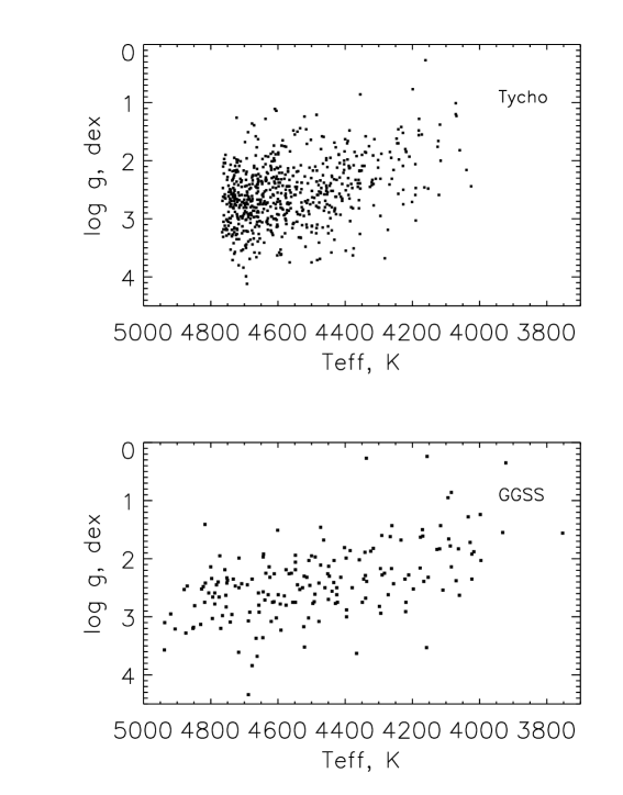
Figure 6: The diagram $T_{eff}$ versus $\log~{}g$ for the Tycho (upper panel) and GGSS (lower panel) samples. The distribution of the two different samples in this diagram illustrates the clustering of the Tycho sample to a more localized region in the T_eff–log g plane when compared to the GGSS sample. The Tycho sample contains a sizable fraction of red giant clump stars, while the GGSS sample consists of giants distributed more uniformly across the first ascent of the red giant branch.

Figure 7: The ratio of Magnesium/Iron abundances versus iron abundances in the control sample of 10 bright stars (filled circles), with the increase in [Mg/Fe] with decreasing [Fe/H] clearly evident. Included in this figure are abundance results from Mishenina et al. (2006) shown with diamonds and the agreement between the two studies is excellent.

Figure 8: The values of [Mg/Fe] versus [Fe/H] in the GGSS and Tycho program stars (dots). The squares and triangles show the abundance results from Reddy et al. (2003, 2006), respectively. The agreement between the abundances derived from the automated analysis developed here when compared to the classical analysis from Reddy et al. (2003, 2006) is very good, demonstrating that the automated analysis produces reliable abundances for Fe and Mg.

References

- Allende Prieto et al. (2008) Allende Prieto C., Sivarani, T., Beers, T.C., Lee, Y. S., et al., 2008, AJ, 136, 2070
- Alonso et al. (1999) Alonso, A., Arribas, S., Martinez-Roger, C. 1999, A&AS, 140, 261
- Bizyaev et al. (2006) Bizyaev, D., Smith, V. V., Arenas, J., Geisler, D., et al. 2006, AJ, 131, 1784
- Brown et al. (1989) Brown, J. A., Sneden, C., Lambert, & D. L., Dutchover, E. 1989, ApJS, 71, 293
- Butler et al. (1996) Butler, R.P., Marcy, G.W., Williams, E., et al. 1996, PASP, 108, 500
- Carlberg et al. (2010) Carlberg J., Majewski S., Patterson R., et al., 2010, submitted to ApJ.
- Castelli & Kurucz (2003) Castelli, F., & Kurucz, R. L. 2003, IAU Symp. 210, Modelling of Stellar Atmospheres, ed. N. Piskunow, W. W. Weiss, & D. F. Gray (Dordrecht: Kluwer), A20
- Catanzarite et al. (2004) Catanzarite J. H, Shao M., & Ciardi D. 2004, BAAS, 2004, 36, 1489
- Ciardi (2004) Ciardi, D. R. 2004, BAAS, 36, 770
- Cochran & Hatzes (1994) Cochran, W. D. & Hatzes, A. P. 1994, Ap&SS, 212, 281
- Frink et al. (2001) Frink, S., Quirrenbach, A., Fischer, D., Röser, S., & Schilbach, E. 2001, PASP, 113, 173
- Fulbright et al. (2006) Fulbright J.P., McWilliam A., Rich R.M., 2006, ApJ, 636, 821
- Gray (1976) Gray D., 2005, The Observation and Analysis of Stellar Photospheres, (New York: Cambridge Univ. Press)
- Hinkle et al. (2000) Hinkle, K., Wallace, L., Valenti, J., & Harmer, D. Visible and Near Infrared Atlas of the Arcturus Spectrum, 3727-9300 Å 2000, (San Francisco: ASP) ISBN: 1-58381-037-4
- Katz et al. (1998) Katz, D., Soubiran, C., Cayrel, R., et al., 1998, A&A, 338, 151
- Kurucz & Bell (1995) Kurucz, R. L., & Bell, B. 1995, Kurucz CD-ROM No. 23 [Cambridge: Smithsonian Astrophysical Observatory]
- Lee et al. (2008a) Lee, Y. S., Beers, T.C., Sivarani, T., Allende Prieto C., et al., 2008, AJ, 136, 2022
- Lee et al. (2008b) Lee, Y. S., Beers, T.C., Sivarani, T., Johnson, J., et al., 2008, AJ, 136, 2050
- Luck & Challener (1995) Luck, R. E. & Challener, S. L., 1995, AJ, 110, 2968
- Majewski et al. (2000) Majewski, S. R., Ostheimer, J. C., Kunkel, W. E., & Patterson, R. J. 2000, AJ, 120, 2550
- McCarthy et al. (2003) McCarthy, J. K., Sandiford, B. A., Boyd, D., & Booth, J. 2003, PASP, 105, 881
- Mishenina et al. (2006) Mishenina, T. V., Bienaym , O., Gorbaneva, T. I., et al. 2006, A&A, 456, 1109
- McWilliam (1990) McWilliam, A., 1990, ApJS, 74, 1075
- Patterson et al. (2001) Patterson, R. J., Majewski, S. R., Slesnick, C. L., et al. Small Telescope Astronomy on Global Scales, ASP Conf. Ser. v.246, IAU Colloquium 183. Ed. by Bohdan Paczynski, Wen-Ping Chen, and Claudia Lemme. San Francisco: Astronomical Society of the Pacific, 2001, p.65
- Press et al. (1992) Press, W.H., Flannery, B.P., Teukolsky, S.A., & Vetterling, W.T., 1992, in ”Numerical Recipes in C: The Art of Scientific Computing” (Second Edition), publ. Cambridge University Press
- Reddy et al. (2003) Reddy, B., Tomkin, J., Lambert, D., & Allende Prieto, C., 2003, MNRAS, 340, 304
- Reddy et al. (2006) Reddy, B., Lambert, D., & Allende Prieto, C., 2006, MNRAS, 367, 1329
- Ramirez & Melendez (2005) Ramirez, I. & Melendez, J. 2005, ApJ, 626, 446
- Skrutskie et al. (2006) Skrutskie, M.F., Cutri, R.M., Stiening, R., et al. 2006, AJ, 131, 1163
- Smith et al. (2000) Smith, V.V., Suntzeff, N. B., Cunha, K., et al. 2000, AJ, 119, 1239
- Sneden (1973) Sneden, C. 1973 Ph.D. thesis, Univ. of Texas, Austin
- Soubiran et al. (2008) Soubiran C., Bienayme O., Mishenina T.V., & Kovtyukh V.V., 2008, A&A480, 91
- Thompson et al. (2005) Thompson R. R., Ciardi D. R., & Catanzarite J. H. 2005, BAAS 37, 455