Detecting and handling outlying trajectories in irregularly sampled functional datasets

Abstract

Outlying curves often occur in functional or longitudinal datasets, and can be very influential on parameter estimators and very hard to detect visually. In this article we introduce estimators of the mean and the principal components that are resistant to, and then can be used for detection of, outlying sample trajectories. The estimators are based on reduced-rank t-models and are specifically aimed at sparse and irregularly sampled functional data. The outlier-resistance properties of the estimators and their relative efficiency for noncontaminated data are studied theoretically and by simulation. Applications to the analysis of Internet traffic data and glycated hemoglobin levels in diabetic children are presented.

t1Supported by NSF Grant DMS-06-04396.

1 Introduction

In many statistical problems the collected data consists of samples of stochastic processes rather than scalars or vectors. Typical examples include human growth curves and circadian rhythms in medicine, time-dependent gene expression profiles in genomics, and spectral curves in chemometrics. Other examples and an overview of the related statistical methodology can be found in Ramsay and Silverman (2005).

As with univariate or multivariate samples, the presence of atypical observations in functional samples tends to complicate the statistical analysis. By atypical observations we mean atypical curves, not just isolated points. To illustrate the problem, consider the following two examples. The first one is a problem on Internet traffic analysis. The data, previously analyzed by Zhang et al. (2007), was collected at the main Internet link of the University of North Carolina campus network during seven consecutive weeks. The traffic is measured in packet counts, every half an hour; the logarithm of the data for the 35 week days is shown in Figure 1(a). Most trajectories, while noisy, show a clear daily pattern: the traffic rises sharply between 7 and 9 a.m., remains at approximately the same level between 9 a.m. and 4 p.m., and goes down again between 4 and 7 p.m. However, there is a clearly atypical curve, a day with unusually low traffic, and another one less conspicuous but still atypical, corresponding to a day when the traffic peaked earlier than usual in the morning. The problems created by these atypical curves, and how to deal with them, will be discussed more extensively in Section 6.

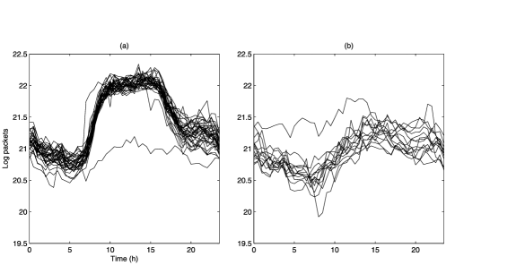
Figure 1: Internet traffic data. Trajectories for (a) 35 week days and (b) 14 weekend days.

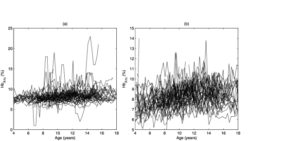
Figure 2: Child diabetes data. Trajectories of $Hb_{A1c}$ levels for (a) 73 females and (b) 66 males.

The second example is more complicated. Figure 2 shows trajectories of glycated hemoglobin levels for diabetic children who underwent treatment at the Children’s Hospital of the University of Zurich. The level of glycated hemoglobin (abbreviated $Hb_{A1c}$) is used to assess the effectiveness of therapy in patients with type-I diabetes mellitus, and to study the long-term effect of the disease on physical and intellectual development [see, e.g., Schoenle et al. (2002)]. One trajectory is clearly out of control in Figure 2(a), but besides that, it is hard to discern any systematic patterns in the data. To complicate the problem, $Hb_{A1c}$ levels are measured at irregular time points, with as few as 2 observations for some individuals. This makes individual smoothing of the trajectories (which would have eased visualization) very hard or even impossible. This example will also be discussed in more detail in Section 6, but it is clear that atypical curves cannot always be detected by visual inspection, and one must rely on methods that can handle outlying curves automatically.

These examples also show that outliers, in the functional sense, are not simply the result of misrecorded data or extreme noise. They correspond to individuals that, for some reason, do not follow the pattern of the majority of the data, and often deserve to be studied more carefully rather than simply discarded. However, these atypical curves must be downweighted at the estimation step, or they may lead to erroneous conclusions for the rest of the population.

This article is organized as follows. Section 2 frames the discussion in a more rigorous statistical setting, as an estimation problem for stochastic processes. Section 3 proposes an outlier-resistant estimation method, and Sections 4 and 5 discuss their asymptotic and finite-sample properties. Section 6 presents a more thorough analysis of the above examples. Available as supplementary material are a Technical Report with proofs and mathematical derivations, and Matlab programs implementing the proposed estimators.

2 Functional data models

The data in the examples above and in similar longitudinal studies can be thought of as discrete observations of continuous-time stochastic processes (or, more generally, of stochastic processes depending on a continuous variable). Usually, the data is observed with random noise:

$$x_{ij}=X_{i}(t_{ij})+\varepsilon_{ij},\qquad j=1,\ldots,m_{i},i=1,\ldots,n,$$ (1)

where $\{X_{i}(t)\}$ are i.i.d. trajectories of the stochastic process of interest, $\{t_{ij}\}$ are the time points where the trajectories are measured, and $\{\varepsilon_{ij}\}$ are independent random errors. It is known [see, e.g., Gohberg, Goldberg and Kaashoek (2003)] that a stochastic process $X\in L^{2}([a,b])$ with $E(\|X\|^{2})<\infty$ admits the expansion (known as Karhunen–Loève decomposition)

$$X(t)=\mu(t)+\sum_{k=1}^{\infty}y_{k}\phi_{k}(t),$$ (2)

where $\mu(t)=\mathrm{E}\{X(t)\}$. The $\phi_{k}$s form a nonrandom orthonormal basis of $L^{2}([a,b])$ and the $y_{k}$s are uncorrelated random variables with zero mean and finite variance. If $\rho(s,t)=\mathrm{cov}\{X(s),X(t)\}$, we have the representation

$$\rho(s,t)=\sum_{k=1}^{\infty}\lambda_{k}\phi_{k}(s)\phi_{k}(t),$$ (3)

where $\lambda_{k}=\mathrm{var}(y_{k})$. If $\rho(s,t)$ is continuous, then the $\phi_{k}$s are also continuous and the series (3) converges uniformly and absolutely. This representation implies that $\lambda_{k}$ is an eigenvalue of $\rho$ with eigenfunction $\phi_{k}$, so the $\phi_{k}$s are called “principal components” and the $y_{k}$s “component scores,” in analogy with multivariate analysis.

To a large extent, the stochastic process $X(t)$ is characterized by $\mu(t)$ and $\rho(s,t)$. Estimating these functions is challenging when the time grid $\{t_{ij}\}$ is irregular or sparse, because it makes individual smoothing of the trajectories very hard or even impossible ($m_{i}$ may be as low as 1 or 2 for some individuals). Some authors that have addressed this problems are Staniswalis and Lee (1998), Yao, Müller and Wang (2005), James, Hastie and Sugar (2000), Gervini (2006), and Yao and Lee (2006). These estimators, however, cannot handle outlying curves like those in the examples of the Introduction. Estimators that do handle outlying curves were proposed by Locantore et al. (1999), Fraiman and Muniz (2001), Cuevas, Febrero and Fraiman (2007), and Gervini (2008), but they can only be applied to individually smoothed trajectories. Estimators that are able to handle outlying curves and can be computed on sparse and irregularly sampled data have not yet been proposed. We present one possible approach in the next section.

3 Reduced-rank $t$-models

The eigenvalues $\lambda_{k}$ in (3) typically decrease to zero very fast, because $\sum_{k=1}^{\infty}\lambda_{k}<\infty$. Therefore, only the leading terms in (2) are of practical relevance, and we can assume

$$X(t)=\mu(t)+\sum_{k=1}^{d}y_{k}\phi_{k}(t)$$ (4)

for some $d$, where $\lambda_{1}\geq\cdots\geq\lambda_{d}>0$. Smoothness of $\mu$ and the $\phi_{k}$s can be built into the model by assuming they are spline functions. That is, we assume $\mu(t)=\bolds{\theta}^{T}\mathbf{b}(t)$ and $\phi_{k}(t)=\bolds{\eta}_{k}^{T}\mathbf{b}(t)$, where $\mathbf{b}(t)\in\mathbb{R}^{p}$ is a spline basis. The observational model implied by (1) and (4) can be succinctly expressed as

$$\mathbf{x}_{i}=\mathbf{B}_{i}\bolds{\theta}+\mathbf{B}_{i}\mathbf{H\bolds\Lambda}^{{1}/{2}}\mathbf{z}_{i}+\sigma\bolds{\varepsilon}_{i},\qquad i=1,\ldots,n,$$ (5)

where $\mathbf{B}_{i}=[b_{k}(t_{ij})]_{(j,k)}$, $\mathbf{H}=[\bolds{\eta}_{1},\ldots,\bolds{\eta}_{d}]$, $\bolds{\Lambda}=\operatorname{diag}(\lambda_{1},\ldots,\lambda_{d})$, $\mathbf{z}_{i}$ is the vector of standardized component scores and $\bolds{\varepsilon}_{i}$ are the standardized measurement errors. If we assume a heavy-tailed distribution for $(\mathbf{z}_{i},\bolds{\varepsilon}_{i})$, outlier-resistant estimators of $\mu$ and the $\phi_{k}$s are obtained automatically. The reason is that, informally speaking, heavy-tailed models “expect” extreme observations, which are then downweighted by the maximum likelihood estimation process.

Specifically, we assume that $(\mathbf{z}_{i},\bolds{\varepsilon}_{i})$ has a joint multivariate $t$ distribution with $\nu$ degrees of freedom, location parameter $\mathbf{0}$ and scatter matrix $\mathbf{I}_{d+m_{i}}$, which we denote by $t_{\nu}(\mathbf{0,I}_{d+m_{i}})$. Then $\mathbf{x}_{i}\sim t_{\nu}(\mathbf{B}_{i}\bolds{\theta,\Sigma}_{i})$, with $\bolds{\Sigma}_{i}=\mathbf{B}_{i}\mathbf{H\bolds\Lambda H}^{T}\mathbf{B}_{i}^{T}+\sigma^{2}\mathbf{I}_{m_{i}}$. The maximum likelihood estimating equations for this model, which are derived in the Technical Report, are the following:

$$\sum_{i=1}^{n}\biggl{(}\frac{\nu+m_{i}}{\nu+s_{i}}\biggr{)}\mathbf{B}_{i}^{T}\bolds{\Sigma}_{i}^{-1}\mathbf{(x}_{i}\mathbf{-B}_{i}\bolds{\theta)} = \mathbf{0},$$ (6)

$$(\mathbf{I}_{d}\mathbf{-JHH}^{T})\mathbf{S}_{n}\bolds{\eta}_{k} = 0,\qquad k=1,\ldots,d,$$ (7)

$$\bolds{\eta}_{k}^{T}\mathbf{S}_{n}\bolds{\eta}_{k} = 0,\qquad k=1,\ldots,d,$$ (8)

$$-\frac{1}{2}\sum_{i=1}^{n}\operatorname{tr}(\bolds{\Sigma}_{i}^{-1})+\frac{1}{2}\sum_{i=1}^{n}\biggl{(}\frac{\nu+m_{i}}{\nu+s_{i}}\biggr{)}(\mathbf{x}_{i}\mathbf{-B}_{i}\bolds{\theta})^{T}\bolds{\Sigma}_{i}^{-2}(\mathbf{x}_{i}\mathbf{-B}_{i}\bolds{\theta})=0,$$ (9)

where

$$\mathbf{S}_{n}=\sum_{i=1}^{n}\biggl{\{}-\mathbf{B}_{i}^{T}\bolds{\Sigma}_{i}^{-1}\mathbf{B}_{i}+\biggl{(}\frac{\nu+m_{i}}{\nu+s_{i}}\biggr{)}\mathbf{B}_{i}^{T}\bolds{\Sigma}_{i}^{-1}\mathbf{(x}_{i}\mathbf{-B}_{i}\bolds{\theta)(x}_{i}\mathbf{-B}_{i}\bolds{\theta)}^{T}\bolds{\Sigma}_{i}^{-1}\mathbf{B}_{i}\biggr{\}},$$

$s_{i}=\mathbf{(x}_{i}\mathbf{-B}_{i}\bolds{\theta)}^{T}\bolds{\Sigma}_{i}^{-1}\mathbf{(x}_{i}\mathbf{-B}_{i}\bolds{\theta)}$ and $\mathbf{J}=[\int b_{i}(t)b_{j}(t)\,dt]_{(i,j)}$. The best linear predictor of $\mathbf{z}_{i}$ is $\mathrm{E}(\mathbf{z}_{i}\mathbf{|x}_{i})=\bolds{\Lambda}^{{1}/{2}}\mathbf{H}^{T}\mathbf{B}_{i}^{T}\bolds{\Sigma}_{i}^{-1}\mathbf{(x}_{i}\mathbf{-B}_{i}\bolds{\theta)}$, and $\hat{\mathbf{z}}_{i}$ is obtained by replacing the model parameters with their estimators.

What makes these estimators robust are the weights $(\nu+m_{i})/(\nu+s_{i})$ that appear in equations (6)–(9). Since $s_{i}$ is the squared Mahalanobis distance between $\mathbf{x}_{i}$ and the expected trajectory $\mathbf{B}_{i}\bolds{\theta}$, atypical trajectories are downweighted and do not seriously affect the estimators. Downweighting is strongest for the Cauchy model ($\nu=1$) and becomes less pronounced as $\nu$ increases. When $\nu\rightarrow\infty$, $(\nu+m_{i})/(\nu+s_{i})\rightarrow 1$ and one obtains the estimating equations for the Normal reduced-rank model [James, Hastie and Sugar (2000)], which gives equal weight to all sample curves and then lacks robustness.

These estimators can be easily computed via the EM algorithm, which is derived in detail in the Technical Report. The recursive steps are the following: given current estimates $\hat{\bolds{\theta}}^{\mathrm{old}}$, $\hat{\bolds{\Xi}}^{\mathrm{old}}$ (where $\bolds{\Xi}=\mathbf{H}\bolds\Lambda^{1/2}$) and $(\hat{\sigma}^{2})^{\mathrm{old}}$, the updates are

$$\hat{\bolds{\theta}}^{\mathrm{new}} = \Biggl{\{}\sum_{i=1}^{n}\biggl{(}\frac{\nu+m_{i}}{\nu+\hat{s}_{i}^{\mathrm{old}}}\biggr{)}\mathbf{B}_{i}^{T}\mathbf{B}_{i}\Biggr{\}}^{-1}\sum_{i=1}^{n}\biggl{(}\frac{\nu+m_{i}}{\nu+\hat{s}_{i}^{\mathrm{old}}}\biggr{)}\mathbf{B}_{i}^{T}(\mathbf{x}_{i}\mathbf{-B}_{i}\mathbf{\hat{\Xi}}^{\mathrm{old}}\hat{\mathbf{z}}_{i}^{\mathrm{old}}),$$

$$\mathrm{vec}(\hat{\bolds{\Xi}}^{\mathrm{new}}) = \Biggl{[}\sum_{i=1}^{n}\biggl{\{}(\hat{\mathbf{V}}_{i}^{\mathrm{old}})^{-1}+\biggl{(}\frac{\nu+m_{i}}{\nu+\hat{s}_{i}^{\mathrm{old}}}\biggr{)}\hat{\mathbf{z}}_{i}^{\mathrm{old}}(\hat{\mathbf{z}}_{i}^{\mathrm{old}})^{T}\biggr{\}}\otimes\mathbf{B}_{i}^{T}\mathbf{B}_{i}\Biggr{]}^{-1}$$

$${}\times\sum_{i=1}^{n}\biggl{(}\frac{\nu+m_{i}}{\nu+\hat{s}_{i}^{\mathrm{old}}}\biggr{)}(\hat{\mathbf{z}}_{i}^{\mathrm{old}}\otimes\mathbf{B}_{i}^{T})(\mathbf{x}_{i}\mathbf{-B}_{i}\hat{\bolds{\theta}}^{\mathrm{old}}),$$

$$(\hat{\sigma}^{2})^{\mathrm{new}} = \frac{1}{\sum_{i=1}^{n}m_{i}}\Biggl{[}\sum_{i=1}^{n}\biggl{(}\frac{\nu+m_{i}}{\nu+\hat{s}_{i}^{\mathrm{old}}}\biggr{)}\|\mathbf{x}_{i}-\mathbf{B}_{i}\hat{\bolds{\theta}}^{\mathrm{old}}-\mathbf{B}_{i}\hat{\bolds{\Xi}}^{\mathrm{old}}\hat{\mathbf{z}}_{i}^{\mathrm{old}}\|^{2}$$

$$\hskip 63.0pt{}+\sum_{i=1}^{n}\operatorname{trace}\{\mathbf{B}_{i}\hat{\bolds{\Xi}}^{\mathrm{old}}(\hat{\mathbf{V}}_{i}^{\mathrm{old}})^{-1}(\hat{\bolds{\Xi}}^{\mathrm{old}})^{T}\mathbf{B}_{i}^{T}\}\Biggr{]},$$

where $\hat{s}_{i}$ and $\hat{\mathbf{z}}_{i}$ are as before, and $\mathbf{V}_{i}=\mathbf{I}_{d}+\bolds{\Xi}^{T}\mathbf{B}_{i}^{T}\mathbf{B}_{i}\bolds{\Xi}/\sigma^{2}$. To obtain $\hat{\mathbf{H}}$ and $\hat{\bolds{\Lambda}}$ from $\hat{\bolds{\Xi}},$ we find the spectral decomposition of $\hat{\bolds{\Xi}}^{T}\mathbf{J}\hat{\bolds{\Xi}}$, say, $\mathbf{UDU}^{T}$ with $\mathbf{U}$ orthogonal and $\mathbf{D}$ diagonal, and set $\hat{\bolds{\Lambda}}=\mathbf{D}$ and $\hat{\mathbf{H}}=\hat{\bolds{\Xi}}\mathbf{UD}^{-1/2}$.

As it is well known, the EM algorithm can take a large number of iterations to converge; but for our estimators each iteration is very fast to compute. Most of the computing time (in our Matlab implementation) is taken up by the recomputation of the spline basis matrix $\mathbf{B}_{i}$ for each $i$ on each iteration, so the computing time grows mostly with $n$ and only marginally with $d$, $p$ or the $m_{i}$s. To give an idea of the computing times involved, each run of the EM algorithm for the simulated data in Section 5, with $n=100$, takes approximately 15 seconds on a common laptop computer with a 2.00GHz Intel Pentium processor.

In practice, the model dimension $d$ is not known a priori, so the computation of the estimators is done in a sequential way. We recommend to begin with a mean-only model ($d=0$), using $\hat{\bolds{\theta}}=\mathbf{0}$ and $\hat{\sigma}^{2}=\sum_{i,j}x_{ij}^{2}/\sum_{i}m_{i}$ as initial estimators for the EM iterations. Then proceed by adding one principal component at a time, using the estimators of the previous $(d-1)$-dimensional model as initial estimators for the $d$-dimensional model. The final dimension $d_{0}$ can be chosen subjectively or objectively. Subjective approaches include choosing a $d$ that yields a small ratio $\hat{\lambda}_{d}/\sum_{k=1}^{d}\hat{\lambda}_{k}$ or a small value of $\hat{\lambda}_{d}$ compared to the noise variance $\hat{\sigma}^{2}$. Objective model selection methods can be based on the maximization of the penalized log-likelihood

$$\sum_{i=1}^{n}\log f(\mathbf{x}_{i}|\hat{\bolds{\theta}},\hat{\mathbf{H}},\hat{\bolds\Lambda})-c_{n}\mathrm{df},$$ (10)

where $f(\mathbf{x}_{i}|\hat{\bolds{\theta}},\hat{\mathbf{H}},\hat{\bolds\Lambda})$ is the $t_{\nu}(\mathbf{B}_{i}\hat{\bolds{\theta}},\hat{\bolds\Sigma}_{i})$ density evaluated at $\mathbf{x}_{i}$, $\mathrm{df}$ are the degrees of freedom of the model, and $c_{n}$ is a constant. Concretely, $c_{n}=1$ defines the AIC criterion and $c_{n}=\log n/2$ the BIC criterion. This approach has been used in the functional data context [Yao, Müller and Wang (2005)] for normally distributed data only, but Shen, Huang and Ye (2004) justify their use for exponential distributions in general. The degrees of freedom of the model are the number of parameters minus the number of orthonormality restrictions. Another objective method that can be used, although in practice it tends to underperform (10), is cross-validation. Cross-validation would maximize

$$\sum_{i=1}^{n}\log f\bigl{(}\mathbf{x}_{i}|\hat{\bolds{\theta}}_{(-i)},\hat{\mathbf{H}}_{(-i)},\hat{\bolds{\Lambda}}_{(-i)}\bigr{)},$$

where $\hat{\bolds{\theta}}_{(-i)}$, $\hat{\mathbf{H}}_{(-i)}$ and $\hat{\bolds{\Lambda}}_{(-i)}$ are the estimators computed without observation $\mathbf{x}_{i}$.

Another aspect that is rather subjective is the choice of basis functions for $\mu(t)$ and $\phi_{k}(t)$, particularly the knot placement and quantity. If a large number of knots is used, placement becomes less important but regularization is necessary. This can be accomplished by adding roughness penalty terms of the form $\alpha\int\{\mu^{\prime\prime}(t)\}^{2}\,dt$ and $\alpha_{k}\int\{\phi_{k}^{\prime\prime}(t)\}^{2}\,dt$ to the log-likelihood function (the resulting modifications of the EM algorithm are straightforward, since these terms are quadratic in the parameters). Selection of the smoothing parameters $\alpha$ and $\alpha_{k}$ can be done, again, either subjectively or objectively. The penalized log-likelihood approach, however, is not as straightforward to implement as before, because the degrees of freedom of the model are not as easy to calculate when the fitted values $\hat{\mathbf{x}}_{i}$ are not linear functions of the data [Ye (1998); Efron (2004)]. Cross-validation, on the other hand, can be implemented as easily as usual despite its shortcomings. Nevertheless, since $\bolds{\theta}$ and the $\bolds{\eta}_{k}$s are model parameters common to all curves, the estimators $\hat{\bolds{\theta}}$ and $\{\hat{\bolds{\eta}}_{k}\}$ “borrow strength” across individuals and then the choice of smoothing parameters is less problematic than if each curve were smoothed individually. This is based on our experience with spline smoothing rather than on formal mathematical results, although for kernel smoothers Yao, Müller and Wang (2005) and Kneip (1994) have indeed established rates of convergence of the estimators and the bandwidths that depend fundamentally on the number of curves $n$ rather than the number of observations per curve $m_{i}$.

4 Asymptotic properties

The distributional assumptions made in Section 3 were just working assumptions to derive robust estimators of $\mu(t)$ and the $\phi_{k}(t)$s. In this section we will study the consistency of the estimators under broader conditions. We will also study their sensitivity to outliers, as quantified by the influence function.

To simplify, let us assume that the individual time grids $\mathbf{t}_{1},\ldots,\mathbf{t}_{n}$ are i.i.d. realizations of a random vector $\mathbf{t}\in\mathbb{R}^{m}$, so $m_{i}=m$ for all $i$. Let $\mathbf{w}=(\mathbf{t},\mathbf{x})$ and let us collect all model parameters in a single vector $\bolds{\xi}=(\bolds{\theta},\bolds{\eta}_{1},\ldots,\bolds\eta_{d},\lambda_{1},\ldots,\lambda_{d},\sigma^{2})$. The estimating equations (6) to (9) can be expressed as a single system of equations $\sum_{i=1}^{n}\bolds{\psi}(\mathbf{w}_{i},\hat{\bolds{\xi}})=\mathbf{0}$ for an appropriate function $\bolds{\psi}(\mathbf{w},\cdot)\dvtx\mathbb{R}^{(p+1)(d+1)}\rightarrow\mathbb{R}^{(p+1)(d+1)}$. Estimators of this type are called $M$-estimators, or sometimes $Z$-estimators [Maronna, Martin and Yohai (2006), Chapter 3; Van der Vaart (1998), Chapter 5]. For such estimators the notion of Fisher consistency is useful. Suppose $\mathbf{w}=(\mathbf{t},\mathbf{x})$ follows model (5) with parameter $\bolds{\xi}=\bolds{\xi}_{0}$, and let $F_{0}$ be the resulting distribution of $\mathbf{w}$. Let $\bolds{\xi}=\bolds{\xi}(F_{0})$ be the solution to the eqnarray $\mathrm{E}_{F_{0}}\{\bolds{\psi}(\mathbf{w},\bolds\xi)\}=\mathbf{0}$. In principle, $\bolds{\xi}(F_{0})$ need not be equal to the true model parameter $\bolds{\xi}_{0}$; if it is, the estimator is said to be Fisher consistent [Maronna, Martin and Yohai (2006), page 67]. It turns out that under some regularity conditions, $M$-estimators $\hat{\bolds{\xi}}$ converge in probability to $\bolds{\xi}(F_{0})$ as $n$ goes to infinity; then, under those regularity conditions, Fisher consistency implies the usual consistency [Van der Vaart (1998), Theorem 5.9].

The next theorem shows that $\hat{\bolds{\theta}}$ and the $\hat{\bolds{\eta}}_{k}$s are Fisher consistent under broad conditions, whereas $\hat{\sigma}^{2}$ and the $\hat{\lambda}_{k}$s are off by a common factor [this is typical of $M$-estimators of scale parameters; see Maronna, Martin and Yohai (2006), Chapter 6.12].

Theorem 1

If $\mathbf{w}=(\mathbf{t},\mathbf{x})$ follows model (5) with parameter $\bolds{\xi}_{0}$, and $\mathbf{(z,\bolds\varepsilon)}$ has a joint spherical distribution, then $\bolds{\xi}(F_{0})=(\bolds{\theta}_{0},\bolds{\eta}_{01},\ldots,\bolds{\eta}_{0d},\beta_{0}\lambda_{01},\break\ldots,\beta_{0}\lambda_{0d},\beta_{0}\sigma_{0}^{2})$ with $\beta_{0}>0$ a factor that depends on the distribution of $(\mathbf{z},\bolds\varepsilon)$ and on $\nu$ but not on the model parameter $\bolds{\xi}_{0}$.

Theorem 1 implies that the estimators of $\mu$ and the $\phi_{k}$s derived under a $t_{\nu}$ distributional assumption on $(\mathbf{z},\bolds\varepsilon)$ are actually Fisher consistent under any spherical distribution of $(\mathbf{z},\bolds\varepsilon)$, including the Normal distribution or a $t_{\nu^{\ast}}$ distribution with $\nu^{\ast}\neq\nu$. The estimators of $\sigma^{2}$ and the $\lambda_{k}$s, although not Fisher-consistent, are off by a common factor $\beta_{0}$, which implies that the ratios $\hat{\lambda}_{d}/\hat{\sigma}^{2}$ and $\hat{\lambda}_{d}/\sum_{k=1}^{d}\hat{\lambda}_{k}$ are Fisher-consistent.

Now we turn our discussion to the outlier sensitivity of the estimators. Outlier sensitivity can be measured by the influence function [Maronna, Martin and Yohai (2006), Chapter 3], which is defined as

$$\operatorname{IF}(\mathbf{w};\hat{\bolds{\xi}},F_{0})=\lim_{\varepsilon\searrow 0}\frac{1}{\varepsilon}\bigl{\{}\bolds{\xi}\bigl{(}(1-\varepsilon)F_{0}+\varepsilon\delta_{\mathbf{w}}\bigr{)}-\bolds{\xi}(F_{0})\bigr{\}},$$

where $\delta_{\mathbf{w}}$ is the point-mass distribution at $\mathbf{w}$. The gross-error sensitivity of $\hat{\bolds{\xi}}$ is defined as $\gamma^{\ast}=\sup_{\mathbf{w}}\|\operatorname{IF}(\mathbf{w};\hat{\bolds{\xi}},F_{0})\|$. Note that for a small contamination proportion $\varepsilon$, the asymptotic bias caused by $\delta_{\mathbf{w}}$ is approximately $\varepsilon\operatorname{IF}(\mathbf{w};\hat{\bolds{\xi}},F_{0})$. Therefore, if $\gamma^{\ast}<\infty$, the bias is bounded regardless of the location of the outliers and the estimator $\hat{\bolds{\xi}}$ is said to be locally robust.

For regular $M$-estimators, it can be shown that $\operatorname{IF}(\mathbf{w};\hat{\bolds{\xi}},F_{0})=-\mathbf{M}^{-1}\bolds{\psi}(\mathbf{w},\break\bolds{\xi}(F_{0}))$, where $\mathbf{M}=\mathrm{E}_{F_{0}}\{\partial\bolds{\psi}(\mathbf{w},\bolds\xi)/\partial\bolds{\xi}^{T}|_{\bolds{\xi}=\bolds{\xi}(F_{0})}\}$ [Maronna, Martin and Yohai (2006), Chapter 3]. Then $\gamma^{\ast}\leq\lambda_{\min}^{-1/2}(\mathbf{MM}^{T})\sup_{\mathbf{w}}\|\bolds{\psi}(\mathbf{w},\bolds\xi(F_{0}))\|$, where$\lambda_{\min}(\mathbf{A})$ denotes the smallest eigenvalue of $\mathbf{A}$, so $\gamma^{\ast}<\infty$ as long as $\mathbf{M}$ is invertible and $\bolds{\psi}(\mathbf{w},\bolds\xi)$ is bounded in $\mathbf{w}$. This is true for our estimating functions $\bolds{\psi}$, so the $t$-model estimators $\hat{\bolds{\xi}}$ are locally robust.

Influence functions are also useful for the computation of asymptotic variances. Under appropriate regularity conditions, $\sqrt{n}(\hat{\bolds{\xi}}-\bolds{\xi}(F_{0}))$ converges in distribution to a $N(\mathbf{0},\mathbf{V})$ with $\mathbf{V}=\mathrm{E}\{\operatorname{IF}(\mathbf{w};\hat{\bolds{\xi}},F_{0})\operatorname{IF}(\mathbf{w};\hat{\bolds{\xi}},F_{0})^{T}\}$ [Van der Vaart (1998), Theorem 5.21]. This result is useful, for instance, to derive asymptotic confidence bands for $\mu(t)$, provided one can obtain a more explicit expression for the $p\times p$ block of $\mathbf{V}$ that corresponds to the asymptotic variance of $\hat{\bolds{\theta}}$. In some cases this is possible, as the next theorem shows.

Theorem 2

If $\mathbf{w}=(\mathbf{t},\mathbf{x})$ follows model (5) and $(\mathbf{z},\bolds\varepsilon)$ has a joint spherical distribution, then $\mathbf{M}$ has a block structure

$$\mathbf{M}=\left[\matrix{\mathbf{M}_{11}&\mathbf{0}\cr\mathbf{0}&\mathbf{M}_{22}}\right]$$

with $\mathbf{M}_{11}\in\mathbb{R}^{p\times p}$ given by

$$\mathbf{M}_{11}=\mathrm{E}_{F_{0}}\biggl{\{}g(\mathbf{w})\mathbf{B}^{T}(\mathbf{t})\frac{1}{\beta_{0}}\bolds{\Sigma}^{-1}(\mathbf{t})\mathbf{B}(\mathbf{t})\biggr{\}},$$

where

$$g(\mathbf{w})=\frac{2}{m}\frac{(\nu+m)s(\mathbf{w})/\beta_{0}}{\{\nu+s(\mathbf{w})/\beta_{0}\}^{2}}-\frac{\nu+m}{\nu+s(\mathbf{w})/\beta_{0}},$$

$\mathbf{B}(\mathbf{t})=[b_{k}(t_{j})]_{(j,k)}$, $\bolds{\Sigma}(\mathbf{t})=\mathbf{B}(\mathbf{t})\mathbf{H}_{0}\bolds{\Lambda}_{0}\mathbf{H}_{0}^{T}\mathbf{B}^{T}(\mathbf{t})+\sigma_{0}^{2}\mathbf{I}_{m}$, $s(\mathbf{w})=\{\mathbf{x}-\bolds{\mu}_{0}(\mathbf{t})\}^{T}\times\break\bolds{\Sigma}^{-1}(\mathbf{t})\{\mathbf{x}-\bolds{\mu}_{0}(\mathbf{t})\}$ and $\bolds{\mu}_{0}(\mathbf{t})=\mathbf{B}(\mathbf{t})\bolds{\theta}_{0}$. Furthermore,

$$\operatorname{IF}(\mathbf{w};\hat{\bolds{\theta}},F_{0})=-\mathbf{M}_{11}^{-1}\biggl{(}\frac{\nu+m}{\nu+s(\mathbf{w})/\beta_{0}}\biggr{)}\mathbf{B}^{T}(\mathbf{t})\frac{1}{\beta_{0}}\bolds{\Sigma}^{-1}(\mathbf{t})\{\mathbf{x}-\bolds{\mu}_{0}(\mathbf{t})\}.$$

From Theorem 2 we see that the asymptotic covariance matrix of $\hat{\bolds{\theta}}$ has the form $\mathbf{M}_{11}^{-1}\mathbf{AM}_{11}^{-1}$, and due to the block structure of $\mathbf{M}$, $\hat{\bolds{\theta}}$ is asymptotically independent of $\{\hat{\bolds{\eta}}_{k}\}$, $\{\hat{\lambda}_{k}\}$ and $\hat{\sigma}^{2}$. The matrices $\mathbf{M}_{11}$ and $\mathbf{A}$ can be estimated by

$$\hat{\mathbf{M}}_{11}=\frac{1}{n}\sum_{i=1}^{n}\hat{g}_{i}\mathbf{B}_{i}^{T}\hat{\bolds{\Sigma}}_{i}^{-1}\mathbf{B}_{i}$$

and

$$\hat{\mathbf{A}}=\frac{1}{n}\sum_{i=1}^{n}\biggl{(}\frac{\nu+m}{\nu+\hat{s}_{i}}\biggr{)}^{2}\mathbf{B}_{i}^{T}\hat{\bolds{\Sigma}}_{i}^{-1}(\mathbf{x}_{i}-\hat{\bolds{\mu}})(\mathbf{x}_{i}-\hat{\bolds{\mu}})^{T}\hat{\bolds{\Sigma}}_{i}^{-1}\mathbf{B}_{i},$$

where

$$\hat{g}_{i}=\frac{2(\nu+m)\hat{s}_{i}}{m(\nu+\hat{s}_{i})^{2}}-\frac{\nu+m}{\nu+\hat{s}_{i}}.$$

Note that, by Theorem 1, $\hat{\bolds{\Sigma}}_{i}$ and $\hat{s}_{i}$ are consistent estimators of $s(\mathbf{w}_{i})/\beta_{0}$ and $\bolds{\Sigma}^{-1}(\mathbf{t}_{i})/\beta_{0}$, so $\hat{\mathbf{M}}_{11}^{-1}\hat{\mathbf{A}}\hat{\mathbf{M}}_{11}^{-1}$ is a consistent estimator of $\mathbf{M}_{11}^{-1}\mathbf{AM}_{11}^{-1}$.

5 Simulation study

5.1 Assessment of parameter estimators

We studied the finite-sample behavior of the estimators by simulation. We were mainly interested in the relative efficiency of the estimators for normally distributed data and in their bias under outlier contamination. Three estimators were considered: the maximum likelihood estimator for (a) the Normal model [James, Hastie and Sugar (2000)], (b) the Cauchy model, which is a $t$-model with $\nu=1$, and (c) the $t$-model with $\nu=5$. As spline basis we chose cubic splines with five equidistant knots. We considered different simulation scenarios (described below) but only part of the results are reported here (Table 1). The rest can be found in the Technical Report.

To assess the efficiency of the estimators, we simulated data from the two-component model

$$x_{ij}=\mu(t_{ij})+\sum_{k=1}^{2}z_{ik}\sqrt{\lambda_{k}}\phi_{k}(t_{ij})+\sigma\varepsilon_{ij},$$ (11)

with $\mu(t)=0$ and $\phi_{k}(t)=\sqrt{2}\sin(k\pi t)$, for $t\in[0,1]$. The component scores $z_{ik}$ and the random errors $\varepsilon_{ij}$ were independent $N(0,1)$ and $\lambda_{1}=1$, $\lambda_{2}=0.5$, $\sigma^{2}=0.25$. Three designs were considered for the $t_{ij}$s: (i) $m=20$ fixed uniformly spaced points in $[0,1]$, (ii) $m=20$ random points (which vary from curve to curve) with uniform distribution in $[0,1]$, and (iii) $m_{i}$ random points with uniform distribution in $[0,1]$, where $m_{1},\ldots,m_{n}$ was a sample from a Poisson random variable with mean 15. The third design is the one that best resembles sparse and irregularly observed data. As sample sizes we took $n=50$, $n=100$ and $n=200$. Each sampling situation was replicated 500 times. Root mean squares of $\|\hat{\mu}-\mu\|$ and $\|\hat{\phi}_{1}-\phi_{1}\|$ are given in Table 1, for grid design (ii) and sample size $n=100$. The relative behavior of the estimators is similar for the other designs and sample sizes, as can be seen in the more detailed results shown in the Technical Report. We see that the $t$-model estimators are generally less efficient than the Normal-model estimators, as expected, but the loss of efficiency is minimal. We also note that the estimators $\hat{\mu}$ were obtained by fitting a mean-only model to the simulated data, whereas the estimators $\hat{\phi}_{1}$ where obtained by fitting a one-component model to the data; therefore, the models were always underspecified, but this did not seem to affect the consistency of the estimators (the boxplots in the Technical Report show that the errors decrease as $n$ increases).

Table 1: Simulation results. Root mean squared errors of different estimators for noncontaminated normal data and outlier-contaminated data

				No contam.		Endogenous contam.				Exogenous contam.
Estim.		Model				10%	20%	30%		10%	20%	30%
$\hat{\mu}$		Normal		0.142		0.427	0.819	1.205		0.367	0.703	1.040
		Cauchy		0.169		0.190	0.247	0.330		0.162	0.184	0.212
		$t_{5}$		0.159		0.183	0.254	0.365		0.153	0.179	0.224
$\hat{\phi}_{1}$		Normal		0.142		1.091	1.331	1.363		0.942	1.265	1.290
		Cauchy		0.165		0.299	0.627	1.006		0.158	0.189	0.220
		$t_{5}$		0.163		0.338	0.673	1.087		0.152	0.183	0.232

To assess the robustness of the estimators, two types of outliers were considered; we call them endogenous and exogenous. Endogenous outliers are curves that belong to the space spanned by $\{\phi_{1},\phi_{2}\}$ just like the rest of the data, only that the component scores $\mathbf{z}_{i}$ follow a different distribution. Exogenous outliers, on the contrary, are curves that do not belong to the space spanned by $\{\phi_{1},\phi_{2}\}$. In these simulations we generated exogenous outliers by taking linear combinations of $\phi_{1}$, $\phi_{2}$ and $\phi_{3}(t)=c\{t(1-t)\}^{1/2}\sin\{2\pi(1+2^{(9-4k)/5})/(t+2^{(9-4k)/5})\}$ with $k=5$ (the so-called “Doppler function,” with $c$ such that $\|\phi_{3}\|=1$). Three contamination proportions were considered for the scenarios described below: $\varepsilon=0.10$, $\varepsilon=0.20$ and $\varepsilon=0.30$. The time grid was generated following the uniform random design (ii), and the sample size was $n=100$. Each scenario was replicated 500 times.

Let us first examine the robustness of $\hat{\mu}$. Endogenous outliers were generated by replacing $\varepsilon n$ component scores $z_{i1}$ with a large constant $K$ (so the outlying curves were virtually identical to $K\sqrt{\lambda_{1}}\phi_{1}$), whereas exogenous outliers were generated by adding $K\sqrt{\lambda_{1}}\phi_{3}$ to $\varepsilon n$ sample curves. We considered two contaminating constants, $K=4$ and $K=8$, but only the results for $K=4$ are reported in Table 1 (the results for $K=8$ are given in the Technical Report). Since the “true” mean for these samples are $\varepsilon K\phi_{1}$ and $\varepsilon K\phi_{3}$, respectively, because $\lambda_{1}=1$, the root mean squared errors should be approximately $\varepsilon K$ for nonrobust estimators. This is exactly what we see in Table 1 for the Normal-model estimator. In contrast, $t$-model estimators show remarkably low biases, even for contamination proportions as high as 30%.

To study the robustness of $\hat{\phi}_{1}$, endogenous outliers were generated by replacing $\varepsilon n/2$ scores $z_{i2}$ with $K\sqrt{\lambda_{2}}$ and $\varepsilon n/2$ with $-K\sqrt{\lambda_{2}}$; exogenous outliers were generated by adding $K\sqrt{\lambda_{1}}\phi_{3}$ to $\varepsilon n/2$ sample curves and subtracting the same quantity to other $\varepsilon n/2$ sample curves. As before, we used $K=4$ and $K=8$ but only report the case $K=4$ here, since the other results are similar. Note that these symmetric contaminations affect $\hat{\phi}_{1}$ but do not affect $\hat{\mu}$, because they alter the covariance structure without changing the mean. In fact, the endogenously contaminated data follows model (11) with $\lambda_{1}^{\ast}=(1-\varepsilon)\lambda_{1}$ and $\lambda_{2}^{\ast}=(1-\varepsilon)\lambda_{2}+\varepsilon\lambda_{2}K^{2}$, so $\lambda_{2}^{\ast}$ can be actually larger than $\lambda_{1}^{\ast}$ if $K$ is big enough, in which case we expect the root mean squared error of a nonrobust estimator to be close to $\|\phi_{2}-\phi_{1}\|=\sqrt{2}$. This is what we observe in Table 1. The exogenously contaminated data also follows model (11) with three components, but the components are not $\phi_{1}$, $\phi_{2}$ and $\phi_{3}$ (because they are not orthogonal). We see in Table 1 that endogenous outliers have a more deleterious effect on the estimators than exogenous outliers. In fact, the $t$-model estimators are practically unaffected by exogenous outliers. Under endogenous contaminations, the performance of the $t$-model estimators deteriorates for large contamination proportions, although they still outperform the Normal-model estimators.

Overall, the conclusion from this Monte Carlo study is that $t$-model estimators are highly resistant to outliers, even for relatively large contamination proportions, and have a high relative efficiency for Normal data. Given that their computational complexity is comparable to that of Normal-model estimators, we think that they are a practical and safer alternative. In particular, we recommend the use of Cauchy-model estimators, since they are the most robust in the $t$ family and are not much less efficient than $t_{5}$-model estimators for Normal data.

5.2 Assessment of model selection criteria

Table 2: Simulation results. Percentage of times AIC and BIC select a two-component model and a three-component model, for Normal and Cauchy estimators and several contamination proportions

		Contamination proportion
$\bolds{n}$	Method	0%	10%	20%	30%
$20$	AIC-Nor	$(99,1)$	$(1,74)$	$(3,65)$	$(6.3,62.3)$
	BIC-Nor	$(99.7,0.3)$	$(1,79.3)$	$(4.7,71.3)$	$(11.3,66.3)$
	AIC-Cau	$(98,2)$	$(74,24.3)$	$(12.3,83.7)$	$(0,87.3)$
	BIC-Cau	$(99.7,0.3)$	$(84.7,15.3)$	$(20.7,78)$	$(0.3,94.7)$
$60$	AIC-Nor	$(100,0)$	$(0.3,60.7)$	$(0.3,53.7)$	$(1.3,62)$
	BIC-Nor	$(100,0)$	$(0.3,62.3)$	$(0.3,55.3)$	$(2,66)$
	AIC-Cau	$(100,0)$	$(79.3,20)$	$(0.3,76)$	$(0,67.7)$
	BIC-Cau	$(100,0)$	$(89.3,10.7)$	$(1,94.7)$	$(0,92)$

We also ran a Monte Carlo study to evaluate the performance of the AIC and BIC criteria for selection of the model dimension $d$. We generated data from the two-component model (11) and from a symmetrically contaminated model with exogenous outliers, as explained above. Since exogenous contamination introduces a spurious third direction of variability, the expected effect on the AIC and BIC criteria is an overestimation of the model dimension.

We compared two types of estimators: the Normal-model estimators and the Cauchy-model estimators. As before, we chose cubic splines with five equidistant knots as spline basis; then $p=9$ and, for the true model with $d=2$, the degrees of freedom are 27. We considered two sample sizes, $n=20$ and $n=60$ (note that in the former case $n$ is less than the degrees of freedom of the true model). The models were fitted in a sequential way, as suggested in Section 3, from $d=0$ to $d=4$. Each sampling situation was replicated 300 times.

The results are summarized in Table 2. We show two outputs: the percentage of the samples for which the right model is selected and the percentage of the samples for which the next model ($d=3$) is selected; the remaining percentage would correspond to the four-dimensional model, since we observed that models with $d<2$ were never selected. For noncontaminated data, it is clear that the criteria have no trouble selecting the right model, neither for Normal nor for Cauchy estimators. For low contamination levels ($\varepsilon=0.10$) the AIC and BIC based on Cauchy estimators select the right model in the vast majority of cases, with the BIC criterion being clearly superior; the nonrobust Normal estimators, in contrast, almost never led to the right choice of model. For larger contamination proportions, even the robust estimators break down; but even then we note that the BIC based on Cauchy-model estimators outperforms the alternatives, since it selects the slightly overspecified model $d=3$ most of the time and very rarely leads to the worst choice $d=4$, in contrast to the other methods. All things considered, we think the BIC based on Cauchy estimators is a recommendable criterion for selection of the number of components.

6 Examples

6.1 Internet traffic

Accurate modeling of Internet traffic data is essential for an efficient allocation of computational resources. In this section we show that just a couple of atypical curves can lead to seriously misleading results. The data, previously analyzed by Zhang et al. (2007), was collected at the main Internet link of the University of North Carolina during seven consecutive weeks (from June 9 to July 25, 2003). The traffic is measured in packet counts, every half hour. The logarithm of the data for week days is shown in Figure 1(a) and for weekend days in Figure 1(b).

Although the data is very noisy, we see that the trajectories follow a regular pattern, which is different for week days than for weekends. Here we analyze only the 35 week days. There is a very clear outlier in Figure 1(a), a curve that actually looks like a weekend trajectory. This curve corresponds to the Fourth of July. A more subtle atypical curve corresponds to June 27, the second day of classes and the last day for late registration for the Second Summer Session. That day the traffic peaked two hours earlier than usual, and also decreased earlier than usual in the afternoon.

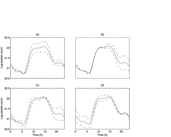
Figure 3: Internet traffic data. Estimators of the mean (—–) and the mean plus ($---$) and minus ($-\cdot-$) a constant times the principal component, for Normal-model estimators [(a), (c)] and Cauchy-model estimators [(b), (d)] of the first [(a), (b)] and second [(c), (d)] principal components.

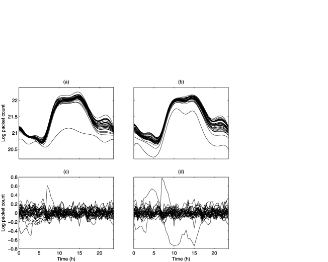
Figure 4: Internet traffic data. Estimated trajectories [(a), (b)] and residuals [(c), (d)] from Normal-model estimators [(a), (c)] and Cauchy-model estimators [(b), (d)].

We estimated the mean and the first two principal components using Normal-model and Cauchy-model estimators based on cubic splines with 10 equispaced knots. The results are shown in Figure 3. Rather than plotting the principal components themselves, we show their effect on the mean, by plotting $\hat{\mu}$ plus/minus a constant times $\hat{\phi}_{k}$. This makes interpretation easier. We see that the mean estimators are similar but the principal components are completely different. The Normal-model estimator of the first component is an amplitude effect (above/below the mean, but parallel to it) and the second component is a shape component (traffic higher than the mean until 3 p.m. and lower than the mean afterward). The first component is clearly dominant, since $\hat{\lambda}_{1}=0.329$ and $\hat{\lambda}_{2}=0.085$. It is very suspicious that these components essentially mimic the two outliers; in fact, July 4 has the largest first component score and June 27 the largest second component score.

On the other hand, the Cauchy-model estimators of the components explain amplitude variability at the end of the day (the first component) and at the beginning of the day (the second component), with the total variability roughly equally split ($\hat{\lambda}_{1}=0.176$ and $\hat{\lambda}_{2}=0.123$). Of course, the fact that the two methods produce different estimators does not automatically imply that the Cauchy-model estimators are better, but a residual analysis confirms this. Cauchy-model estimators produce smaller residual norms $\|\mathbf{x}_{i}-\hat{\mathbf{x}}_{i}\|$ than Normal-model estimators for 25 of the 35 observations. The median residual norm for the Cauchy fit is $0.556,$ while for the Normal fit it is $0.592$. Figure 4 shows individual predictors and residuals; undoubtedly, Cauchy-model estimators offer an overall better fit (except for the Fourth of July outlier). Normal-model estimators show a particularly poor fit for the Internet traffic between 0 and 6 a.m.

6.2 Child diabetes study

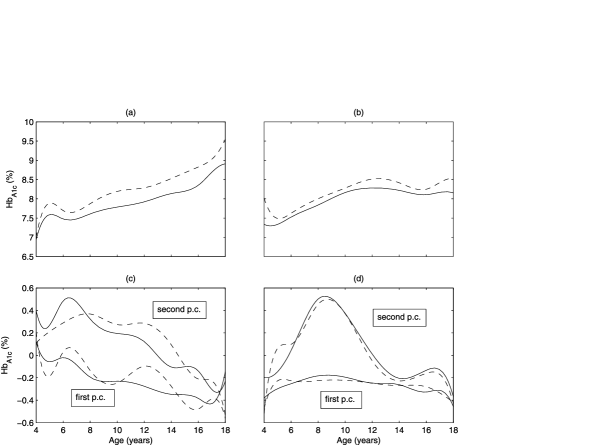
Figure 5: Child diabetes data. Estimated means [(a), (b)] and leading principal components [(c), (d)] of $Hb_{A1c}$ trajectories for females [(a), (c)] and males [(b), (d)], using Normal (dashed line) and Cauchy (solid line) maximum likelihood estimators.

Glycated hemoglobin ($Hb_{A1c}$) levels are often used as a measure of average plasma glucose concentration over certain periods of time. Figure 2 shows trajectories of $Hb_{A1c}$ levels for diabetic children who underwent treatment at the Children’s Hospital of the University of Zurich. The profiles are very irregularly sampled and noisy. For girls, the minimum number of observations per trajectory is 2, the median 33 and the maximum 55; for boys, the minimum number of observations per trajectory is 2, the median 33 and the maximum 56. For such irregular data individual smoothing is impractical, even impossible for the shortest trajectories. The presence of at least one outlying curve is plain to see in Figure 2(a), although it is hard to tell by visual inspection if there are any other outliers.

We estimated the mean and the principal components for each sex, using Normal and Cauchy maximum likelihood estimators. Cubic splines with 6 equispaced knots were used as basis functions. The BIC based on Normal-model estimators selects a three-component model for both sexes, while the BIC based on Cauchy-model estimators selects a four-component model; however, in the latter case $\hat{\lambda}_{4}$ is very small compared to $\hat{\sigma}^{2}$ and the other $\hat{\lambda}$s, so we settled for a three-component model. Figure 5 shows the estimators of the mean and the two leading components (the third one is omitted for better visibility). For males, both methods produce similar estimators, but for females the differences are striking. The Normal-model estimators not only overestimate the mean but also provide a very irregular estimator of the first principal component; the estimator of the second component is also substantially different from the Cauchy-model estimator.

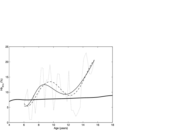
Figure 6: Child diabetes data. Outlying trajectory (dotted line), Cauchy-model estimator of the mean (thick solid line), and fitted trajectory using Cauchy-model predictor (thin solid line) and Normal-model predictor (dashed line).

The trajectory with the largest mean squared residual for girls is shown in Figure 6. This is a patient whose diabetes level was clearly out of control. We see that the Normal-model estimator provides a somewhat better fit for this curve than the Cauchy estimator, but this is at the expense of a poorer fit for the rest of the individuals. The mean squared residual of this observation is 22.6 for the Normal fit and 24.8 for the Cauchy fit. However, the three quartiles of the mean squared residuals for the whole sample are 0.18, 0.40 and 0.63 for the Cauchy fit, and 0.24, 0.43 and 0.71 for the Normal fit, so the Cauchy fit is better overall. Another confirmation of this is that the Normal-model estimators obtained after eliminating the outlying trajectory are very similar to the Cauchy estimators.

7 Conclusion and discussion

As we have shown in Section 6, outlying curves do occur in longitudinal and functional datasets. When individual smoothing is feasible, they can be handled by the robust methods alluded to in Section 2. But when the data is sparse and irregular, individual smoothing is unfeasible and methods that employ the raw data must be used. One possible approach has been presented in this article. The idea of using $t$ models to derive robust estimators is not new to Statistics [see, e.g., Lange, Little and Taylor (1989)], but those procedures were specifically developed for low dimensional multivariate data. They cannot be applied “off the shelf” to functional or longitudinal data, where the dimension of the covariance matrix often exceeds the sample size. However, an adaptation of the reduced-rank approach of James, Hastie and Sugar (2000) provides a way to implement $t$-model estimators in the functional data context. The approach we have followed is the simplest one, which is to assume that $(\mathbf{z}_{i},\bolds{\varepsilon}_{i})$ in (5) is jointly $t$ distributed, and, as a result, the $\mathbf{x}_{i}$s themselves have a multivariate $t$ distribution. But other approaches are possible. For instance, it could be assumed that $\mathbf{z}_{i}$ and $\bolds{\varepsilon}_{i}$ have multivariate $t$ distributions but are independent, or even that each $\varepsilon_{ij}$ has an independent $t$ distribution. Unfortunately, none of these assumptions imply that the $\mathbf{x}_{i}$s have a multivariate $t$ distribution, which complicates the theoretical study of the estimators’ properties and the derivation of the EM algorithm. Nevertheless, these alternatives are worth further research.

Technical Report and Matlab code [doi]10.1214/09-AOAS257SUPP [url]http://lib.stat.cmu.edu/aoas/257/supplement.zip .zip The pdf file contains proofs, technical derivations and more detailed simulation results not given in the paper. The zip file contains Matlab programs implementing the EM algotihm for Normal and $t$ reduced-rank models.

References

- (1) Cuevas, A., Febrero, M. and Fraiman, R. (2007). Robust estimation and classification for functional data via projection-based depth notions. Comput. Statist. 22 481–496. \MR2336349
- (2) Efron, B. (2004). The estimation of prediction error: Covariance penalties and cross-validation. J. Amer. Statist. Assoc. 99 619–632. \MR2090899
- (3) Fraiman, R. and Muniz, G. (2001). Trimmed means for functional data. Test 10 419–440. \MR1881149
- (4) Gervini, D. (2006). Free-knot spline smoothing for functional data. J. Roy. Statist. Soc. Ser. B 68 671–687. \MR2301014
- (5) Gervini, D. (2008). Robust functional estimation using the median and spherical principal components. Biometrika 95 587–600. \MR2443177
- (6) Gohberg, I., Goldberg, S. and Kaashoek, M. A. (2003). Basic Classes of Linear Operators. Birkhäuser, Basel. \MR2015498
- (7) James, G., Hastie, T. G. and Sugar, C. A. (2000). Principal component models for sparse functional data. Biometrika 87 587–602. \MR1789811
- (8) Kneip, A. (1994). Nonparametric estimation of common regressors for similar curve data. Ann. Statist. 22 1386–1472. \MR1311981
- (9) Lange, K. L., Little, R. J. A. and Taylor, J. M. G. (1989). Robust statistical modeling using the t distribution. J. Amer. Statist. Assoc. 84 881–896. \MR1134486
- (10) Locantore, N., Marron, J. S., Simpson, D. G., Tripoli, N., Zhang, J. T. and Cohen, K. L. (1999). Robust principal components for functional data (with discussion). Test 8 1–28. \MR1707596
- (11) Maronna, R. A., Martin, R. D. and Yohai, V. J. (2006). Robust Statistics. Theory and Methods. Wiley, New York. \MR2238141
- (12) Ramsay, J. O. and Silverman, B. W. (2005). Functional Data Analysis, 2nd ed. Springer, New York. \MR2168993
- (13) Schoenle, E. J., Schoenle, D. Molinari, L. and Largo, R. H. (2002). Impaired intellectual development in children with type 1 diabetes mellitus: Association with high glycated hemoglobin and gender, but not with severe hypoglycemic episodes. Diabetologia 45 108–114.
- (14) Shen, X., Huang, H.-C. and Ye, J. (2004). Adaptive model selection and assessment for exponential family distributions. Technometrics 46 306–317. \MR2082500
- (15) Staniswalis, J. G. and Lee, J. J. (1998). Nonparametric regression analysis of longitudinal data. J. Amer. Statist. Assoc. 93 1403–1418. \MR1666636
- (16) Van der Vaart, A. W. (1998). Asymptotic Statistics. Cambridge Univ. Press. \MR1652247
- (17) Yao, F., Müller, H.-G. and Wang, J.-L. (2005). Functional data analysis for sparse longitudinal data. J. Amer. Statist. Assoc. 100 577–590. \MR2160561
- (18) Yao, F. and Lee, T. C. M. (2006). Penalized spline models for functional principal component analysis. J. Roy. Statist. Soc. Ser. B 68 3–25. \MR2212572
- (19) Ye, J. (1998). On measuring and correcting the effects of data mining and model selection. J. Amer. Statist. Assoc. 93 120–131. \MR1614596
- (20) Zhang, L., Marron, J. S., Shen, H. and Zhu, Z. (2007). Singular value decomposition and its visualization. J. Comput. Graph. Statist. 16 833–854. \MR2412485