Absence of a Periodic Component in Quasar $z$-Distribution

Abstract

Since the discovery of quasars in papers often appeared and appear the assertions that the redshift quasar distribution includes a periodic component with the period $\Delta z=0.063$ or 0.11. A statement of such kind, if it is correct, may manifest the existence of a far order in quasar distribution in cosmological time, that might lead to a fundamental revision all the cosmological paradigm. In the present time there is a unique opportunity to check this statement with a high precision, using the rich statictics of 2dF and SDSS catalogues ($\sim$ 85000 quasars). Our analysis indicates that the periodic component in distribution of quasar redshifts is absent at high confidence level.

Keywords: (cosmology:) large-scale structure of Universe, (galaxies:) quasars: general, catalogues, methods: data analysis.

1 Introduction

As early as the first hundred galaxies with active nuclei and quasars have been discovered, the attempts to reveal the periodicity in their redshift distribution have been made. For example, the presence of peaks at $z_{*}=0.061\cdot n$, where $n$ is the integer, for the distribution of 73 objects with non-thermal optical continuum and $z<0.6$ was mentioned in Burbidges papers (Burbidge & Burbidge, 1957; Burbidge, 1968). They used this fact to confirm their hypothesis concerning the non-cosmological origin of the lines redshift in active galaxy and quasar spectra. However, the other interpretations are also possible. Particularly, some authors discussed the effect of the influence of occurence of several strong emission lines typical for quasars (Mg II, 2800 Å; C III, 1900 Å; C IV, 1550 Å; Ly_α, 1216 Å), in the range of spectral observations ($\lambda>3300$ Å), which might emulate the ”humps” in $N_{q}(z)$ distribution (see, for example Karitskaya & Komberg (1970)).

In the following years in a numbre of papers (e.g. Jaakkola (1971); Tifft (1976, 1989); Tifft & Cocke (1993); Tifft (1996); Bell & Comean (2003); Narlikar & Arp (1993); Bell et al. (2004)) the authors reported about the observed quantization of the redshifts in spectra of near S-galaxies, which satisfies the ”Tifft series”:

$$\Delta v_{r}=2^{-(D+B/9)},$$ (1)

where $v_{r}$ is the radial velocity expressed in light velocity units, $D$ and $B$ are the integers.

In Khodyachikh (1979, 1990) papers the cyclical changes of statisticslly brightest quasars were revealed in V filter, using the argument

$$x\equiv\ln\left(1+z\right)$$ (2)

with $\Delta x\approx 0.19$ period. In Khodyachikh (1988) paper the dependence of a numbre of powerful radiopulsars has been plotted against $x$ variable. In the centimeter wavelength region the cyclic changes were revealed with periods 0.12, 0.19 and 0.38. It is interesting that much later in Ryabnikov et al. (2001a, b) papers, the similar result was obtained after the analysis of the redshist distribution of $\sim$ 800 absorption lines in spectra of bright AGN with $0.10<z<3.7$. The authors mentioned that a separate analysis of $N_{abs}(z)$ distribution in different celestial hemispheres indicates that the phase of periodicity is conserved. They interpreted such unexpected result as a sign of existence of an oscillatory regime in the Universe expansion and then as a presence of a large scale cellular structure in the distribution of the absorption systems in quasar spectra. In Ryabnikov & Kaminker (2010) paper the presence of the periodic structure is considered on the basis of the absorbtion lines.

In Karlsson (1971, 1974) papers the peaks in $N_{q}(z)$ distribution with the step $\Delta x\approx 0.19$ were considered on the basis of 574 quasar data. In papers Burbidge & Napier (2001) and Bell & McDiarmid (2006) on the basis of a gross sample the peaks in $N_{q}(z)$ distribution were mentioned at $z_{*}=0.062$, 0.3, 0.6, 0.96, 1.41, 1.96, 2.63, 3.45. These peak values satisfied the ”Bell series”, Bell (2002):

$$z_{*}=0.062\cdot\left(10N-M\right),$$ (3)

where $N$ and $M$ take on integer values (see the corresponding table in Bell (2002)). The initial series redshift coincides with the first term of the main Tifft series with $D=4$, $B=0$, that corresponds to the velocity $\approx$ 18600 km/s.

It is obvious that in order to confirm such a non-standard conclusion concerning the distinctive features in redshift quasar distribution it is necessary to analyse a much wider statistical information, which is included in the catalogues 2dF (Croom et al., 2004) and SDSS (Shnider et al., 2003). And the papers with analysis of such kind have really appeared. Thus, for example, in Tang & Zhang (2005) paper there was reported the result of analysis of 290 quasars sample (the same sample as used in Karlsson and Burbidge papers) and the periodicity with the step $\Delta x=0.081$ has been confirmed at $3\,\sigma$ level. However, the analysis of larger samples (22497 quasars in 2dF and 46420 in SDSS-5), presented in the same paper Tang & Zhang (2005), did not reveal any periodicity. From this they drew a conclusion that the point is in non-homogeneity of small samples and the selection effects, which the small samples are exposed. So, the problem, seemingly, can be abandoned,

However, there is a numbre of papers where the authors, analyzing the large catalogues, find the arguments for the existence of the periodicity in $N_{q}(z)$ distribution. For example, in Bell & McDiarmid (2006) paper, according to SDSS data 6 peaks in the power spectrum were detected with the step $\Delta z=0.65$ at $z_{*}=1.2$, 1.8, 2.4, 3.1 and 3.7. And in papers Hartnett & Hirano (2007a), Hartnett (2007b) on the basis of 2dF and SDSS catalogues the authors reported the presence of the ”humps” through $\Delta z=0.0102,0.0246,0.0448$, that assuming that $H_{0}=72$ km/c Mpc corresponds to the cells of 44, 102 and 176 Mpc. Except that, the distribution $N_{q}(z)$ is represented in the form $z_{*}=0.062\cdot n$, where $n=3,4,5,6,10,20$ (Hartnett, 2007c). Nevertheless, in Tang & Zhang (2005) paper the arguments have been expressed for the fact that SDSS catalogue may include a periodic component because of the selection effects.

However, it is clear that the analysis of different quasar samples leads the authors to unlike conclusions, concerning the existence or non-existence of a far order in $N_{q}(x)$ distribution. At present there is a unique possibility to check with high precision the hypothesis about the possible periodicity, using the rich statistics of 2dF and SDSS catalogues ($\sim$ 85 thousand quasars). So, it is worth to consider this problem more accurately, and this is the goal of the paper.

2 Observational data and periodicity extraction methods

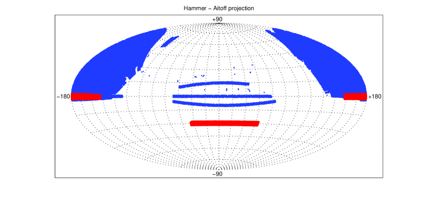
Figure 1: Covering the celestial sphere by 2dF (dark grey) and SDSS (light grey) catalogues.

In the current paper we used two catalogues: 2dF (Croom et al., 2004) (22272 objects) and SDSS (Shnider et al., 2003) (63255 objects, release 7). Covering the celestial sphere by these catalogues is shown in Fig. 1. As one can see, these regions are overlapped and the density of the objects in 2dF catalogue is as much as one order larger than in SDSS. In last (seventh) release of SDSS catalogue some ”gaps” have been filled with respect to the previous one, and as a result of it the sample become more homogeneous.

The periodicity criterion is a function $K(T)$ of the data and a trial period $T$, which takes on ”large” values when the data includes the periodic component with period $T$, otherwise its values are ”small”.

To investigate the periodicity we used four different criteria. The first of them and, apparently, the most familiar one is the Rayleigh criterion:

$$K_{1}(T)=\frac{2}{N}\left[\left(\sum\limits_{i=1}^{N}\sin\frac{2\pi x_{i}}{T}\right)^{2}+\left(\sum\limits_{i=1}^{N}\cos\frac{2\pi x_{i}}{T}\right)^{2}\right],$$ (4)

where $x_{i}$ are the values of the variable $x$ from (2) for each quasar with redshift $z$, $N$ – total amount of objects, and $T$ – trial period in the units of $x$. Three other criteria analyse the structure of assumed periodic component (for variable stars it is called a light curve). For that purpose we subdivide the assumed trial period $T$ in $m$ parts (each of $T/m$ length), calculate the phase of each quasar and add the unity in the appropriate $m$-th part of the period. As a result we obtain a histogram, which indicates the numbre of quasars that drop in each of $m$ parts of assumed period $T$. Three criteria for that histogram analysis are the variety of the epoch superposition method and can be written as:

$$K_{2}(T)=\frac{m}{N}\sum\limits_{j=1}^{m}\left(n_{j}-\frac{N}{m}\right)^{2},$$ (5)

$$K_{3}(T)=1-\frac{\min n_{j}}{\max n_{j}},$$ (6)

$$K_{4}(T)=\frac{m}{N}\left[\sum\limits_{j=1}^{m-1}\left(n_{j+1}-n_{j}\right)^{2}+\left(n_{1}-n_{m}\right)^{2}\right],$$ (7)

where $m$ is the number of parts (bins, intervals) in which the trial period is subdivided and $n_{j}\;\;(j=1,2,\dots,m)$ – the numbre of quasars which drop in the appropriate $j$-th part of a trial period. If the periodic component in the data is absent, then all $m$ bins should have approximately the same values. On the contrary, if the data contain a periodic component they should strongly differ. All criteria have different sensitivity and reveal different aspects of periodicity, therefore it is not unreasonable to use all of them for a more reliable detection of the periodicity.

If we use the stochastic data, the mean criteria values are: $MK_{1}=2$, $MK_{2}=9$, $MK_{4}=20$, that corresponds to the accepted value $m=10$, and the dispersions are, respectively, $DK_{1}=4$, $DK_{2}=18$, $DK_{4}=120$. It means that if the criterion $K_{1}$ takes on the value $K_{1}=7$, then it exeeds the random signal level by $2.5\,\sigma$. To calculate the theoretical values of $MK_{3}$ and $DK_{3}$ we should make use the formulas from Gurin et al. (1988). Statistical properties of the criteria are considered in Gurin et al. (1992) paper.

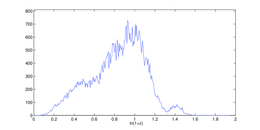
Figure 2: Quasar distribution over redshift in the SDSS catalogue. The absciss axis corresponds to the quantity $x\equiv\ln(1+z)$ from (2). The ordinate axis shows the numbre of objects in the $x$-direction interval of 0.004 width.

3 Analysis of quasar distribution over redshift

The quasar distribution over redshift $z$ in two catalogues shown in Fig. 2 and 3. Analysing the plots one can draw a conclusion that the SDSS catalogue is more representative in the region of large and small $x$ ($x<0.4$ and $x>1.3$). Four large maxima in the SDSS quasar distribution near $x_{*}\approx 0.5,0.8,1$ 1.4 can be explained by the selection effect (the redshift $z$ is detected using four spectral lines) and are not related to a periodicity. In general, we may observe in the plots some oscillations with smaller periods, which might appear a weak periodic component after a detailed analysis.

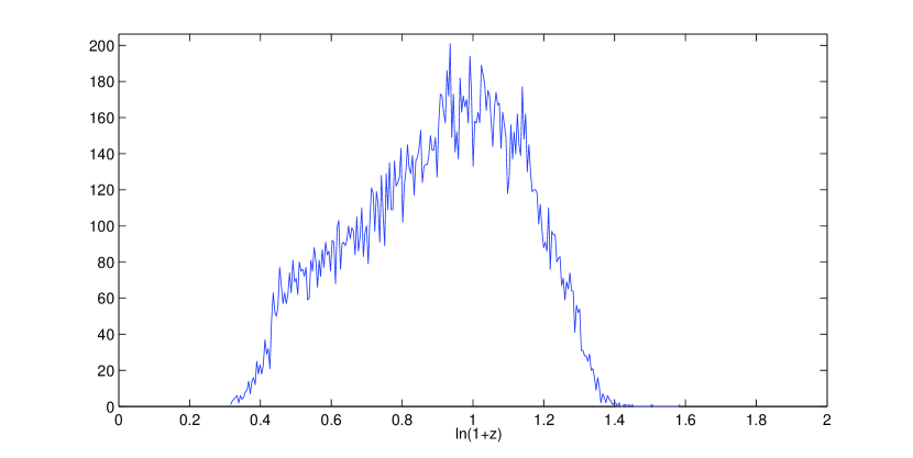
Figure 3: Quasar distribution over redshift in the 2dF catalogue. The ordinate axis shows the numbre of objects in the $x$-direction interval of 0.0046 width.

The result of application of criteria (4) – (7) to the SDSS catalog in the interval $0<T<0.14$ is presented in Fig. 4. As it follows from the plots, all the criteria yield the similar results with diffrent confidence degree, therefore we use below the Rayleigh criterion only. The spectrum of the 2dF catalogue shown in Fig. 5.

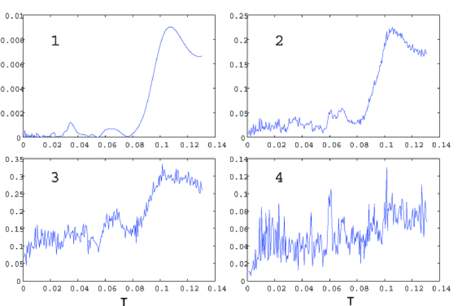
Figure 4: Spectrum $K(T)$ from (4) – (7) of quasar distribution $N_{q}(T)$ according to the SDSS catalogue. The absciss corresponds to the trial period $T$. The criterion numbre marked in each panel.

Figure 5: Spectrum $K_{1}(T)$ of the quasar distribution according to the 2dF catalogue. Absciss corrsponds to a corresponding period $T$ over coordinate $x$ from (2). Rayleigh criterion (4) used.

Indeed, in the SDSS spectrum there are maxima, mentioned by some authors, near the values $T=\Delta x=0.063$ and $0.11$, though at a low confidence level. Except that there is one more, even higher maximum at $T=0.035$. In the 2dF spectrum one can see the maxima at $T\approx 0.034,\>0.083$ and $0.11$, but the maximum near 0.064 is very low. Using approach of such a kind we cannot define exact values of the confidence levels, because for this purpose we have to simulate a stochastic sample with the same parameters as the one in Fig. 2. This approach, however, allows us to detect position of the periodic component with highest possible precision. Note that the values of the periodicity criterion in this case are very small. It is clear enough, because we try to extract a weak periodic component against a background of a very strong continuous signal, similar to investigating of behaviour of sea waves when measuring depth of an ocean.

To increase the extraction reliability one should use another way. Namely: one should cut the background component and consider only the oscillations of $\Delta N_{q}(x)$ with respect to a background. One can do it, subdividing the sample in narrow $z$-intervals and analysing the numbre of quasars in these narrow intervals, i.e. essentially, averaging the distribution inside each interval. The distributions in Fig.  2 and  3 are prepared using this technique. As a ”background” we consider the mean value of 5 neighbouring intervals, where the interval of interest is in the middle. In all cases we consider the absciss as the middle of the appropriate interval. The result of application of this procedure to the SDSS catalogue are presented in Fig. 6 (for the 2dF catalogue the result looks the same). If the periodic component in the distribution does exist it should be distinguished in the plot even by naked eye. However the plot in Fig. 6 hardly looks like a periodic one and rather looks like a noise. It confirms the spectrum of the plot, calculated according to Rayleigh crinterion and shown in Fig. 7. As it is known (Gurin et al., 1992) the mean value of the Rayleigh criterion for the stochastic data equals to 2 and the mean standard deviation is also 2. Indeed, we can reveal in Fig. 7 two maxima at $x_{*}=0.063$ and 0.111, however the confidence level does not seem to be high. One can only mark that these components are slightly stand out against their neighbours, but the reliable detection of the periodicity cannot be confirmed. Thus, according to the available data we cannot draw a conclusion that the periodic component in $\ln(1+z)$ coordinate presents in the quasar distribution over redshift.

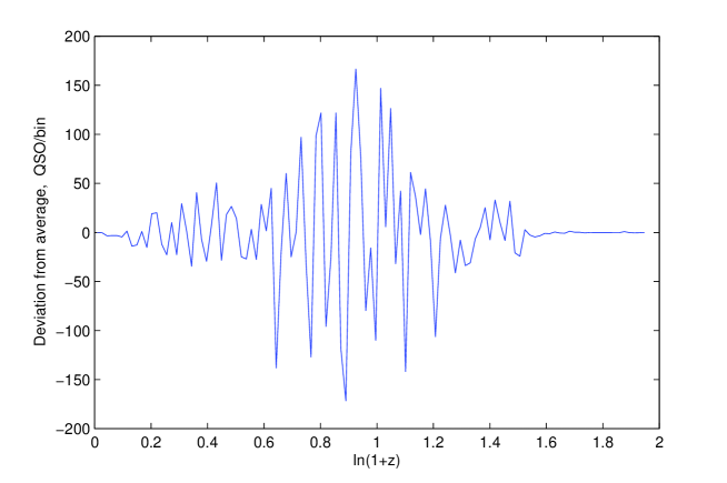
Figure 6: Quasar distribution over redshift in the SDSS catalogue after subrtacion the background component.

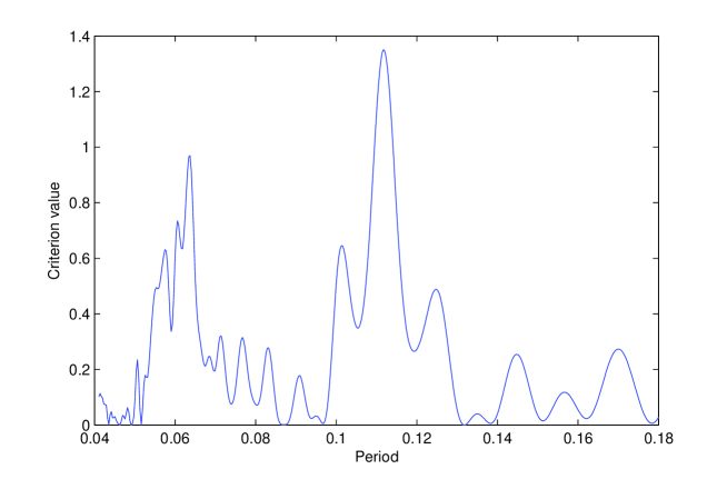
Figure 7: Quasar distribution spectrum $K_{1}(T)$ in the SDSS catalogue after subtaction the background component.

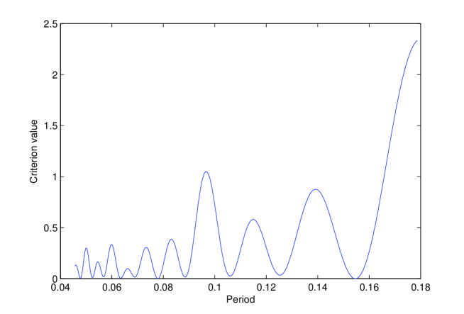
Figure 8: Quasar distribution spectrum $K_{1}(T)$ according to the SDSS catalogue. The absciss axis corresponds to the period, espressed in the units of geodesic cosmological distance $R(z)$ from (8).

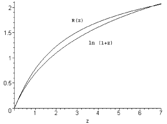
Figure 9: The plots of functions $R(z)$ from (8) for $\Omega_{m}=0.28$, $\Omega_{\Lambda}=0.72$ and $\ln(1+z)$. When $z\to\infty$ the function $R(z)$ tends to a horizontal asymptote, but $\ln(1+z)$ goes to infinity. The lines cross at $z=6.60517$.

It, however, does not mean that the periodicity is absent for other coordinate choice as well. It is possible to check the periodic properties for other variables. The most interesting variable here is

$$R(z)=\int\limits_{0}^{z}\frac{dz}{\sqrt{\Omega_{m}\left(1+z\right)^{3}+\Omega_{\Lambda}}},$$ (8)

which has the physical meaning of the geodesic cosmological distance. Note that when $z\to\infty$   $R(z)$ tends to a constant value, i.e. to the horizon. According to current measurements $\Omega_{m}+\Omega_{\Lambda}\approx 1$, $0.25<\Omega_{m}<0.3$. The spectrum in $R(z)$-coordinate for the SDSS catalogue after subtraction the background using the procedure described above, and applying to the residual the Rayleigh criterion (4) is shown in Fig. 8. Again, near the values $z_{*}=0.06$ and 0.1 there are the maxima in the spectrum, but with a low confidence level. Moreover, it seems that the maximum at $z_{*}=0.06$ is undistinguishable from the near maxima, and the peak at $z_{*}\approx 0.1$ is only slightly higher than its neighbours. In general the plots in Fig. 7 and Fig. 8 do not differ enough from each other.

The point here is that the functions $R(z)$ and $\ln(1+z)$ closely approximate each other. Both functions are shown in Fig. 9 and in the interval for $0<z<7$ they differ not more than 10%, i.e. exactly in the interval in which drop the quasars in the SDSS catalogue. For large $z$ the functions behave in different ways: when $z\to\infty$ $R(z)$ tends to a horizontal asymptote (for $\Omega_{m}=0.28$ and $\Omega_{\Lambda}=0.72$ this value is 3.3988), while $\ln(1+z)$ tends to infinity.

Thus, in this case we also cannot confirm that in the quasar distribution over redshift exists a periodic component.

4 Discission and conclusions

From the analysis above one can draw a conclusion that the reliable extraction of a regular periodic component in the the quasar distribution over redshift is failed. However, the rippling of the quasar density, probably, esceeds the statitical errors.

Most likely we deal with a cellular structure. The individual cell walls, appearing on the line of sight make their contribution to the numbre of quasars at fixed $z$. The quasar $z$-distribution structure of such a kind is not already stochastic, though it retains many properties of the random distribution. In particular, the dispersion may appear greater than theoretical, because an average amount of quasars inside the ”bubble” and in its walls differs significantly from the averaged numbre of the quasars in the unit volume.

Except that at present time the SDSS catalogue covers less than a quarter of the celestial sphere, i.e. the quasar distribution over the celestial sphere in it is essentially non-homogeneous. Further development of the catalogue should smooth all irregularities in $z$-distribution. As a result the spectral features in the distribution will be revealed at gradually decreasing confidence level.

Summarizing our discussion, one can draw a conclusion that the periodic component in quasar $z$-distribution is absent at high confidence level.

5 Acknowledgements

One author (S.R.) is very grateful to Prof. E.Starostenko, Dr. O.Sumenkova and Dr. R.Beresneva for the possibility of fruitful working under this problem. The autors are grateful to Prof. A.Doroshkevich and Dr. V.Strokov for their attention to the problem and useful discusstions and Dr. P.Ivanov for help.

The work was supported by Russian Foundation for Basic Resiarch, grants 09-02-12163, 11-02-00857 and Federal program ”Scientific and scientific-educational personnel of innovational Russia”, State contract $\Pi$-1336.

References

- Bell (2002) Bell M.P., 2002, ApJ, 566, 705, astro-ph/0208320.
- Bell & Comean (2003) Bell M.B., Comean S.P., astro-ph/0305112.
- Bell et al. (2004) Bell M.B., Comean S.P., Kussell D.G., astro-ph/0407591.
- Bell (2004) Bell M.P., astro-ph/0403089.
- Bell & McDiarmid (2006) Bell M.P., Mc. Diarmid D., 2006, ApJ, 648, 140, astro-ph/0603169.
- Burbidge & Burbidge (1957) Burbidge G.R., Burbidge E.M., 1957, ApJ, 148, L107.
- Burbidge (1968) Burbidge G.R., 1968, ApJ, 154, 41.
- Burbidge & Napier (2001) Burbidge G.R., Napier W.H., 2001, Asronom. J., 121, 21.
- Croom et al. (2004) Croom S., Smith R., Boyle B. et al., 2004, MNRAS, 349, 1397.
- Gurin et al. (1988) Gurin L.S., Belyaeva N.P., Bisnovatyi-Kogan G.S., Boudnik E.Yu., Boudnik S.V., 1988, ASpS, 147, 307.
- Gurin et al. (1992) Gurin L.S., Repin S.V. Samoilova Yu.O., 1992, Preprint IKI RAS, Pr-1846.
- Hartnett & Hirano (2007a) Hartnett J.G., Koichi Hirano, arXiv/0711.4885.
- Hartnett (2007b) Hartnett J.G., arXiv/0712.3833v3.
- Hartnett (2007c) Hartnett J.G., arXiv/0712.3833v1.
- Jaakkola (1971) Jaakkola T., 1971, Nature, 234, 534.
- Karitskaya & Komberg (1970) Karitskaya E.A., Komberg B.V., 1970, Astronomy Reports, 47, 41.
- Karlsson (1971) Karlsson K.G., 1971, A&A, 13, 333.
- Karlsson (1974) Karlsson K.G., 1974, A&A, 58, 237.
- Khodyachikh (1979) Khodyachikh M.F., 1979, Astronomy Reports, 56, 1174.
- Khodyachikh (1990) Khodyachikh M.F., 1990, Astronomy Reports, 67, 218.
- Khodyachikh (1988) Khodyachikh M.F., 1988, Kinematics and physics of Celestial Bodies, 4, 53.
- Narlikar & Arp (1993) Narlikar J., Arp H., 1993, ApJ, 405, 51.
- Ryabnikov et al. (2001a) Ryabnikov A.I., Kaminker A.D., Varshalovich D.A., 2001, Astronomy Reports Letters, 27, 643.
- Ryabnikov et al. (2001b) Ryabnikov A.I., Kaminker A.D., Varshalovich D.A., 2001, MNRAS, 376, 1838.
- Ryabnikov & Kaminker (2010) Ryabnikov A.I., Kaminker A.D., arXiv/1007.2487v1.
- Shnider et al. (2003) Shnider D., Fan X., Hall P.B. et al., 2003, Astron. J., 126, 2579.
- Tang & Zhang (2005) Tang S.M., Zhang S.N., 2005, ApJ, 633, 41, astro-ph/0506366.
- Tifft (1976) Tifft W.G., 1976, ApJ, 206, 38.
- Tifft (1989) Tifft W.G., 1989, ApJ, 336, 128.
- Tifft & Cocke (1993) Tifft W.G., Cocke W.J., 1993, BAAS, 25, 796.
- Tifft (1996) Tifft W.G., 1996, ApJ, 468, 491.