Improving the precision of classification trees

Abstract

Besides serving as prediction models, classification trees are useful for finding important predictor variables and identifying interesting subgroups in the data. These functions can be compromised by weak split selection algorithms that have variable selection biases or that fail to search beyond local main effects at each node of the tree. The resulting models may include many irrelevant variables or select too few of the important ones. Either eventuality can lead to erroneous conclusions. Four techniques to improve the precision of the models are proposed and their effectiveness compared with that of other algorithms, including tree ensembles, on real and simulated data sets.

T1This material is based upon work partially supported by U.S. Army Research Office Grants W911NF-05-1-0047 and W911NF-09-1-0205.

1 Introduction

Since the appearance of the AID and THAID algorithms aid , thaid , classification trees have offered a unique way to model and visualize multi-dimensional data. As such, they are more intuitive to interpret than models that can be described only with mathematical equations. Interpretability, however, ensures neither predictive accuracy nor model parsimony. Predictive accuracy is the probability that a model correctly classifies an independent observation not used for model construction. Parsimony is always desirable in modeling—see, for example, McCullagh and Nelder glmbook , page 7—but it takes on increased importance here. A tree that involves irrelevant variables is not only more cumbersome to interpret but also potentially misleading.

Many of the early classification tree algorithms, including THAID, CART cart and C4.5 c45 , search exhaustively for a split of a node by minimizing a measure of node heterogeneity. As a result, if all other things are equal, variables that take more values have a greater chance to be chosen. This selection bias can produce overly large or overly small tree structures that obscure the importance of the variables. Doyle doyle73 seems to be the first to raise this issue, but solutions have begun to appear only in the last decade or so. The QUEST quest and CRUISE cruise algorithms avoid the bias by first using F and chi-squared tests at each node to select the variable to split on. CTree party uses permutation tests. Other approaches are proposed in NSP04 , LS06 and SBA07 .

Unbiasedness alone, however, guarantees neither predictive accuracy nor variable selection efficiency. To see this, consider some data on the mammography experience (ME) of 412 women from Hosmer and Lemeshow HL00 , pages 264–287. The class variable is ME, with 104 women having had a mammogram within the last year (ME${}={}$1), 74 having had one more than a year ago (ME${}={}$2), and 234 women not having had any (ME${}={}$3). [The ME codes here are different from the source; they are chosen to reflect a natural ordering.] Table 1 lists the five predictor variables and the values they take. Hosmer and Lemeshow fitted a polytomous logistic regression model for predicting ME that includes all five predictor variables, but with SYMP and DETC in the form of indicator variables $I(\mathtt{SYMP}\leq 2)$ and $I(\mathtt{DETC}=3)$.

Table 1: Variables in mammography data

Name	Description	Values
ME	Mammography experience	1 (within 1 year), 2 (more
		than 1 year), 3 (never)
SYMP	You do not need a mammogram unless you	1 (strongly agree), 2
	develop symptoms	(agree), 3 (disagree), 4
		(strongly disagree)
PB	Perceived benefit of mammography	5–20 (lower values indicate
		greater benefit)
HIST	Mother or sister with history of breast cancer	0 (no), 1 (yes)
BSE	Has anyone taught you how to examine your	0 (no), 1 (yes)
	own breasts?
DETC	How likely is it that a mammogram could find	1 (not likely), 2 (somewhat
	a new case of breast cancer?	likely), 3 (very likely)

Let $C(i|j)$ denote the cost of misclassifying as class $i$ an observation whose true class is $j$. Because the ME values are ordered, we set $C(i|j)=|i-j|$ for $i,j=1,2,3$. Figure 1 shows the QUEST and CRUISE models. Each leaf node is colored white, light gray or dark gray as the predicted value of ME is 1, 2 or 3, respectively. The QUEST tree is too short; it splits only once and does not predict class 1. Note that class 1 constitutes less than 18% of the sample and that the Hosmer–Lemeshow model HL00 , page 277, Table 8.10, does not predict class 1 too. Another reason that the QUEST tree is shorter than the CRUISE tree is because the latter tests for pairwise interactions at each node, whereas the former does not. Thus, CRUISE can uncover more structure than QUEST.

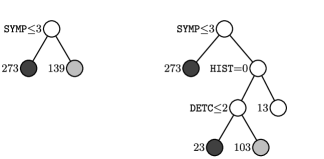
Figure 1: QUEST (left) and CRUISE (right) classification trees for mammography data. At each intermediate node, an observation goes to the left branch if and only if the condition shown there is satisfied. Leaf nodes classified as class 1, 2 and 3 are colored white, light gray, and dark gray, respectively. The number on the left of each leaf node is the sample size.

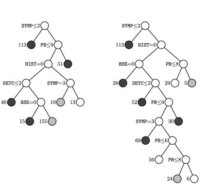
Figure 2: RPART (left) and J48 (right) classification trees for mammography data. At each intermediate node, an observation goes to the left branch if and only if the condition shown there is satisfied. Leaf nodes classified as class 1, 2 and 3 are colored white, light gray and dark gray, respectively. The number on the left of each leaf node is the sample size.

Figure 2 shows the corresponding RPART rpart and J48 weka trees. RPART is an implementation of CART in R and J48 is an implementation of C4.5 in JAVA. The two trees have much more structure, but the J48 tree reminds us that the comprehensibility of a tree structure diminishes with increase in its size. Further, there is a hint of over-fitting in the repeated and nonmonotonic splits on PB at the bottom of the J48 tree. It is difficult to tell which tree model has higher or lower predictive accuracy than the Hosmer and Lemeshow model. Empirical studies have shown that the predictive accuracy of logistic regression is often as good as that of classification trees for small sample sizes LLS00 but that C4.5 is more accurate as the sample size increases PPS03 . (Note: all the trees discussed in this article are pruned according to their respective algorithms. Trees constructed by the new methods to be described are pruned using CART’s cost-complexity method with ten-fold cross-validation.)

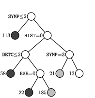
Figure 3: Tree for mammography data using the S method. At each intermediate node, an observation goes to the left branch if and only if the condition shown there is satisfied. Leaf nodes classified as class 1, 2 and 3 are colored white, light gray and dark gray, respectively. The number on the left of each leaf node is the sample size.

Our goal here is to introduce and examine four techniques for constructing tree models that are parsimonious and have high predictive accuracy. We do this by controlling the search for local interactions, employing more effective variable and split selection strategies, and fitting nontrivial models in the nodes. The first technique limits the frequency of interaction tests, performing them only if no main effect test is significant. Besides saving computation time, this reduces the chance of selecting variables of lesser importance. The second technique utilizes a two-level split search when a significant interaction is found. This allows greater advantage to be taken of the information gained from interaction tests. The third technique considers linear splits on pairs of variables, if no main effect or interaction test is significant at a node. This can sometimes produce large gains in predictive accuracy as well as reduction in tree size. The fourth technique fits a nearest-neighbor or a kernel discriminant model, using one or two variables, at each node. This is useful in applications where neither univariate nor linear splits are effective. The result of applying the first three techniques to the mammography data is given in Figure 3. Its model complexity is in between that of CRUISE and QUEST on one hand, and that of RPART and C4.5 on the other.

The rest of this article is organized as follows. Section 2 discusses why and how we control the search for interactions and illustrates the solution with an artificial example. Section 3 introduces linear splits on pairs of variables and motivates the solution with a real example. Section 4 presents simulation results to show that the selection bias of our method is well controlled. Section 5 describes the use of kernel and nearest-neighbor models on pairs of variables to fit the data in each node and demonstrates their effectiveness with yet another example. Section 6 compares the predictive accuracy, tree size and execution time of the algorithms on forty-six data sets. Section 7 examines the effect of using tree ensembles and compares the results with Random Forest randomforest01 . Section 8 concludes the discussion.

2 Controlled search for local interactions

The brevity of the QUEST tree in Figure 1 is attributable to its split selection strategy. At each node, QUEST evaluates the within-node (i.e., local) main effect of each predictor variable by computing an ANOVA $p$-value for each noncategorical variable and a Pearson chi-squared $p$-value for each categorical variable. Then it selects the variable with the smallest $p$-value to split the node. Although successful in avoiding selection bias, QUEST is insensitive to (local) interaction effects within the node. If the latter are strong and local main effects weak, the algorithm can select the wrong variable. The weakness does not necessarily lead to reduced predictive accuracy, however, because good splits may be found farther down the tree—this explains why algorithms with selection biases can still yield models with good predictive accuracy.

CRUISE searches over a larger number of splits at each node by including tests of interactions between all pairs of predictors. If there are $K$ predictor variables, CRUISE computes $K$ main effect $p$-values and $K(K-1)/2$ interaction $p$-values and splits the node on the variable associated with the smallest $p$-value. Because there are usually more interaction tests than main effect tests, the smallest $p$-value often comes from the former. As a result, CRUISE may select a variable with a weak main effect even though there are other variables with stronger ones. Further, if the most significant $p$-value is from an interaction between two variables, CRUISE chooses the variable with the smaller main effect $p$-value and then searches for a split on that variable alone.

To see that this can create difficulties, consider an extreme example where there are two classes and two predictor variables, $X_{1}$ and $X_{2}$, distributed on a square as in Figure 4. The square is divided equally into four sub-squares with one class located in the two sub-squares on one diagonal and the other class in the other two sub-squares. The optimal classification rule first splits the space into two equal halves at the origin using either $X_{1}$ or $X_{2}$ and then splits each half into two at the origin of the other variable. Since this requires a two-level search, CRUISE will likely require many more splits to accurately classify the data.

Figure 4: Class 1 observations uniformly distributed in the white squares and class 2 observations uniformly distributed in the gray squares.

The above problems can be solved by making two adjustments. First, to prevent the interaction tests from overwhelming the main effect tests, we carry out the former only when no main effect test achieves a specified level of significance. Second, we perform a two-level search for the split points whenever a significant interaction is found. These steps are given in detail below, after the introduction of some necessary notation.

Let $J$ denote the number of classes in the training sample and $J_{t}$ the number of classes in node $t$. Let $N_{j}$ denote the number of class $j$ cases in the training sample and $N=\sum_{j}N_{j}$. Let $N_{j}(t)$ and $N(t)$ denote the corresponding sample sizes in $t$, and let $\pi(j)$ be the prior probability for class $j$. The value of $\pi(j)$ may be specified by the user or it can be estimated from the data, in which case it is $N_{j}/N$. The estimated probability that a class $j$ observation will land in node $t$ is $p(j,t)=\pi(j)N_{j}(t)/N_{j}$. Define $p(t)=\sum_{j}p(j,t)$ and $p(j|t)=p(j,t)/p(t)$. The Gini impurity at $t$ is defined as $g(t)=\sum_{i\neq j}p(i|t)p(j|t)$.

2.1 Variable selection

Following CRUISE, we use Pearson chi-squared tests to assess the main effects of the predictor variables. For a noncategorical predictor variable, we discretize its values into three or four intervals, depending on the sample size and the number of classes in the node. But we do not convert the chi-squared values to $p$-values as CRUISE does. Instead, for degrees of freedom (d.f.) greater than one, we use the Wilson–Hilferty wh31 approximation to transform each chi-squared value to a standard normal deviate and then use its inverse transformation to convert it to a chi-squared value with one d.f. This technique, which is borrowed from GUIDE guide , avoids the difficulties of computing very small $p$-values. The detailed procedure is as follows.

Procedure 2.1.

Main effect chi-squared statistic for $X$ at node $t$:

1. [2]

2. If $X$ is a categorical variable:

   1. [(b)]

   2. Form a contingency table with the class labels as rows and the categories of $X$ as columns.

   3. Let $\nu$ be the degrees of freedom of the table after deleting any rows and columns with no observations. Compute the chi-squared statistic $\chi^{2}_{\nu}$ for testing independence. If $\nu>1$, use the Wilson–Hilferty approximation twice to convert $\chi^{2}_{\nu}$ to the 1-d.f. chi-squared

      $$W_{M}(X)=\max\biggl{(}0,\biggl{[}\frac{7}{9}+\sqrt{\nu}\biggl{\{}\biggl{(}\frac{\chi^{2}_{\nu}}{\nu}\biggr{)}^{1/3}-1+\frac{2}{9\nu}\biggr{\}}\biggr{]}^{3}\biggr{)}.$$ (1)

3. If $X$ is a noncategorical variable:

   1. [(b)]

   2. Compute $\bar{x}$ and $s$, the mean and standard deviation, respectively, of the values of $X$ in $t$.

   3. If $N(t)\geq 20J_{t}$, divide the range of $X$ into four intervals with boundary values $\bar{x}$ and $\bar{x}\pm s\sqrt{3}/2$. Otherwise, if $N(t)<20J_{t}$, divide the range of $X$ into three intervals with boundary values $\bar{x}\pm s\sqrt{3}/3$. If $X$ has a uniform distribution, these boundaries will yield intervals with roughly equal numbers of observations.

   4. Form a contingency table with the class labels as rows and the intervals as columns.

   5. Follow step 1(b) to obtain $W_{M}(X)$.

Discretization in step 2(b) is needed to permit application of the chi-squared test. Although the boundaries are chosen for reasons of computational expediency, our empirical experience indicates that the particular choice is not critical for its purpose, namely, unbiasedness in variable selection. Note that the boundaries are not used as split points; a search for the latter is carried out separately in Algorithm 2.2 below.

We apply the same idea to assess the local interaction effects of each pair of variables, using Cartesian products of sets of values for the columns of the chi-squared table.

Procedure 2.2.

Interaction chi-squared statistic for a pair of variables $X_{1}$ and $X_{2}$ at node $t$:

1. [3.]

2. If $X_{i}$ ($i=1,2$) is noncategorical, split its range into two intervals ($A_{i1},A_{i2}$) at the sample mean $\bar{x}$ if $N(t)<45J_{t}$, or three intervals ($A_{i1},A_{i2},A_{i3}$) at the points $\bar{x}\pm s\sqrt{3}/3$, if $N(t)\geq 45J_{t}$. If $X_{i}$ ($i=1,2$) is categorical, let $A_{ik}$ denote the singleton set containing its $k$th value.

3. Divide the $(X_{1},X_{2})$-space into sets $B_{k,m}=\{(x_{1},x_{2})\dvtx x_{1}\in A_{1k},x_{2}\in A_{2m}\}$, for $k,m=1,2,\ldots.$

4. Form a contingency table with the class labels as rows and $\{B_{k,m}\}$ as columns. Compute its chi-squared statistic and use (1) to transform it to a 1-d.f. chi-squared value $W_{I}(X_{1},X_{2})$.

To control the frequency with which interaction tests are carried out, we put a Bonferroni-corrected significance threshold on each set of tests and carry out the interaction tests only if all main effects are not significant. Let $\chi^{2}_{\nu,\alpha}$ denote the upper-$\alpha$ quantile of the chi-squared distribution with $\nu$ d.f. The algorithm for variable selection can now be stated as follows.

Algorithm 2.1 ((Variable selection)).

Let $K>1$ be the number of nonconstant predictor variables in the node. Define $\alpha=0.05/K$ and $\beta=0.05/\break\{K(K-1)\}$:

1. [3.]

2. Use Procedure 2.1 to find $W_{M}(X_{i})$ for $i=1,2,\ldots,K$.

3. If $\max_{i}W_{M}(X_{i})>\chi^{2}_{1,\alpha}$, select the variable with the largest value of $W_{M}(X_{i})$ and exit.

4. Otherwise, use Procedure 2.2 to find $W_{I}(X_{i},X_{j})$ for each pair of predictor variables:

   1. [(b)]

   2. If $\max_{i\neq j}W_{I}(X_{i},X_{j})>\chi^{2}_{1,\beta}$, select the pair with the largest value of $W_{I}(X_{i},X_{j})$ and exit.

   3. Otherwise, select the $X_{i}$ with the largest value of $W_{M}(X_{i})$.

2.2 Split set selection

After Algorithm 2.1 selects a variable $X$ at node $t$, we need to find a set of $X$-values to form the split $t=t_{L}\cup t_{R}$, where $t_{L}$ and $t_{R}$ denote the left and right subnodes of $t$. Let $p_{L}$ and $p_{R}$ denote the proportions of samples in $t$ going into $t_{L}$ and $t_{R}$, respectively. We seek the split that minimizes the weighted sum of Gini impurities

$$p_{L}g(t_{L})+p_{R}g(t_{R}).$$ (2)

Let $n$ be the number of distinct values of $X$ in $t$. If $X$ is noncategorical, there are $(n-1)$ possible splits, with each split point the mean of two consecutive order statistics. If $X$ is categorical, the number of possible splits is $(2^{n-1}-1)$, which grows exponentially with $n$. If $J=2$, however, we use the following short-cut to reduce the search on the categorical variable to $(n-1)$ splits. It is a special case of a more general result proved in cart , Section 9.4.

Theorem 2.1

Suppose that $J=2$ and that $X$ is a categorical variable taking $n$ distinct values. Let $r(a)$ denote the proportion of class 1 observations among those with $X=a$. Let $a_{1}\prec a_{2}\prec\cdots\prec a_{n}$ be an ordering of the $X$ values such that $r(a_{1})\leq r(a_{2})\leq\cdots\leq r(a_{n})$. Given any set $A$, let the observations be split into two groups $t_{L}=\{X\in A\}$ and $t_{R}=\{X\notin A\}$. The set $A$ that minimizes the function $p_{L}g(t_{L})+p_{R}g(t_{R})$ is $A_{i}=\{a_{1},a_{2},\ldots,a_{i}\}$ for some $i=1,2,\ldots,n-1$.

If $X$ is noncategorical, we carry out an exhaustive search for the best split of the form $X\leq c$, with $c$ being the midpoint of two consecutive order statistics. If $X$ is categorical, an exhaustive search is done only if $n\leq 11$ or if $J=2$ (using the above shortcut). Otherwise, a restricted search is performed as follows:

1. [2.]

2. If $J\leq 11$ and $n>20$, divide the observations in $t$ into $n$ groups according to the categorical values of $X$ and find the class that minimizes the misclassification cost in each group. Map $X$ to a new categorical variable $X^{\prime}$ whose values are the minimizing class labels. Carry out an exhaustive search for a split on $X^{\prime}$ and re-express it in terms of $X$.

3. If $J>11$ or $n\leq 20$, transform the categorical values into 0–1 dummy vectors and apply linear discriminant analysis (LDA) to them to find the largest discriminant coordinate $X^{\prime\prime}$. Find the best split on $X^{\prime\prime}$ and then re-express it in terms of $X$. This technique is employed in Loh and Vanichsetakul fact .

The complete details are given as Procedure .1 in the Appendix.

What to do if Algorithm 2.1 selects a pair of variables $X_{1}$ and $X_{2}$, say? Then the split search is more complicated, because the best split on $X_{1}$ may depend on how $X_{2}$ is subsequently split. Similarly, the best split on $X_{2}$ should consider the best subsequent splits on $X_{1}$. Suppose that $t$ is split first by one variable into $t_{L}$ and $t_{R}$, and that $t_{L}$ is split into $t_{\mathit{LL}}$ and $t_{\mathit{LR}}$, and $t_{R}$ into $t_{\mathit{RL}}$ and $t_{\mathit{RR}}$, by the other variable. Let $p_{\mathit{LL}}$, $p_{\mathit{LR}}$, $p_{\mathit{RL}}$ and $p_{\mathit{RR}}$ denote the proportions of samples in $t_{\mathit{LL}}$, $t_{\mathit{LR}}$, $t_{\mathit{RL}}$ and $t_{\mathit{RR}}$, respectively. We select the split $t_{L}$ that minimizes

$$p_{\mathit{LL}}g(t_{\mathit{LL}})+p_{\mathit{LR}}g(t_{\mathit{LR}})+p_{\mathit{RL}}g(t_{\mathit{RL}})+p_{\mathit{RR}}g(t_{\mathit{RR}})$$ (3)

over $t_{\mathit{LL}}$, $t_{\mathit{LR}}$, $t_{\mathit{RL}}$ and $t_{\mathit{RR}}$.

Because this requires a two-level search, we restrict the number of candidate splits to keep computation under control. Let $m_{0}$ be a user-specified number so that only splits yielding at least $m_{0}$ cases in each subnode are permitted. For splits on noncategorical variables $X_{k}$, define $f=\min(100N^{-1},1)$. Let $\lfloor\cdot\rfloor$ be the greatest integer function and let

$$d=\min\{\max(\lfloor fN(t)\rfloor,9),N(t)-2m_{0}+1\}$$

be the number of split points to be evaluated. Clearly, $d<100$. Let $x_{k}(i)$ denote the $i$th order statistic of $X_{k}$. The set of restricted split points on $X_{k}$ are the members of the set

$$S_{k}=\{x_{k}(i_{1}),x_{k}(i_{2}),\ldots,x_{k}(i_{d})\},$$ (4)

where $i_{j}=m_{0}+\lfloor j(N(t)-2m_{0})/(d+1)\rfloor$ and $j=1,2,\ldots,d$. Technical details of the search, covering the cases where 0, 1 or 2 variables are categorical, are given in Procedures .2–.4 in the Appendix. The entire split selection procedure can be stated as follows:

Algorithm 2.2 ((Split selection)).

1. [3.]

2. Apply Algorithm 2.1 to the data in $t$ to select the split variable(s).

3. If one variable is selected and it is categorical, use Procedure .1 to split $t$ on that variable.

4. If one variable is selected and it is noncategorical, search through all mid-points, $c$, of the ordered data values for the split $t_{L}=\{X\leq c\}$ that minimizes (2).

5. If two variables are selected, apply Procedure .2, .3 or .4 to split $t$, depending on whether zero, one or two of the variables are categorical.

The power of this algorithm is best demonstrated by an artificial example. We simulate one thousand observations, each randomly assigned with probability 0.5 to one of two classes. Each class is uniformly distributed in the alternating squares of a $4\times 4$ chess board in the $(X_{1},X_{2})$-plane. The left side of Figure 5 shows one realization, with 520 observations from class 1 and 480 from class 2. We add eight independently and uniformly distributed noise variables. The ideal classification tree should split on $X_{1}$ and $X_{2}$ only and have 16 leaf nodes. C4.5 and CTree yield trees with no splits and hence misclassify 480 observations each. RPART gives a tree with 13 leaf nodes, but splits on $X_{1}$ or $X_{2}$ only three times and misclassifies 347 observations. QUEST misclassifies 27 with a 46-leaf tree. CRUISE splits on $X_{1}$ or $X_{2}$ most of the time and misclassifies 3, but because it does not perform two-level searches, the tree is still large with 29 leaf nodes. Our algorithm splits on $X_{1}$ and $X_{2}$ exclusively and yields a 19-leaf tree that misclassifies 4 observations; its classification regions are shown on the right side of Figure 5.

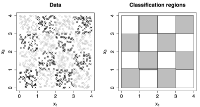
Figure 5: Data (left) and classification regions (right) for the S method.

3 Linear splits

Although univariate splits (viz. splits on one variable at a time) are best for interpretation, greater predictive accuracy can sometimes be gained if splits on linear combinations of variables are allowed. CART uses random search to find linear splits, while CRUISE and QUEST use LDA; see also cline08 , CK03 , tabu03 , YA05 . Nonlinear splits have been considered as well fan08 , LDK05 .

To appreciate the necessity for linear splits, consider some data on fish from Finland obtained from the Journal of Statistics Education data archive (www.amstat.org/publications/jse/datasets/fishcatch.txt). See SASUG and cruise2v for prior usage of these data. There are seven species (classes) in the sample of 159 fish. Their class labels (in parentheses), counts and names are as follows: (1) 35 Bream, (2) 11 Parkki, (3) 56 Perch, (4) 17 Pike, (5) 20 Roach, (6) 14 Smelt and (7) 6 Whitefish. Table 2 lists the seven predictor variables. The data are challenging for univariate splits because the three length variables are highly correlated. For example, Figure 6 shows that it is hard to separate the classes using only univariate splits on length2 and length3. A split along the direction of the data points, however, can separate class 1 (bream) cleanly from the rest.

Table 2: Predictor variables for fish data

weight	Weight of the fish (in grams)
length1	Length from the nose to the beginning of the tail (in cm)
length2	Length from the nose to the notch of the tail (in cm)
length3	Length from the nose to the end of the tail (in cm)
height	Maximal height as a percentage of length3
width	Maximal width as a percentage of length3
sex	Male or female

The CRUISE 2V algorithm cruise2v does well here because it fits a linear discriminant model to a pair of noncategorical variables in each node. We propose instead to keep the node models simple, but use LDA to find splits on two variables at a time. The restriction to two variables permits each split to be presented graphically. It also reduces the impact of missing values—the more variables are involved in a split, the fewer the number of complete cases for its estimation. To prevent outliers from having undue effects on the estimation of the split direction, we trim them before application of LDA in the following procedure. As before, we use chi-squared tests to select the variables for each linear split.

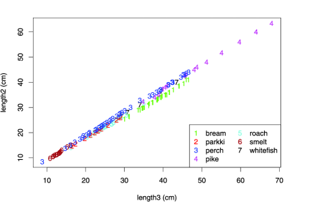
Figure 6: Plot of length2 versus length3 for fish data.

Procedure 3.1.

Discriminant chi-squared statistic. Let $X_{1}$ and $X_{2}$ be two noncategorical variables to be used in a linear split of node $t$:

1. [3.]

2. For class $j$ ($j=1,2,\ldots,J$) and each $X_{i}$ ($i=1,2$), compute the class mean $\bar{x}_{i,j}$ and class standard deviation $s_{i,j}$ of the samples in $t$.

3. Let $S_{j}$ denote the set of class $j$ samples in $t$ lying in the rectangle $|X_{i}-\bar{x}_{i,j}|\leq 2s_{i,j}$ for $i=1,2$.

4. Find the larger linear discriminant coordinate $Z$ from the observations in $S_{1}\cup\cdots\cup S_{J}$.

5. Project the data in $t$ onto the $Z$-axis and compute their $Z$-values.

6. Apply Procedure 2.1 to the $Z$-values to find the one-d.f. chi-squared value $W_{L}(X_{1},X_{2})$.

Although linear splits are more powerful than univariate splits, it is unnecessary to employ a linear split at every node. We see from Figure 6, for example, that almost all the smelts (class 6) can be separated from the other species (except for one misclassified perch) by a univariate split on length2 or on length3 at 14 cm. Therefore, we should invoke linear splits only if the main effect and interaction chi-squared tests are not significant, and then only if the linear split itself is significant. This differs from the linear split options in CART, CRUISE and QUEST, which always split on linear combinations of all the predictors. The next algorithm replaces Algorithms 2.1 and 2.2, if linear splits are desired.

Algorithm 3.1 ((Split selection with the linear split option)).

Let $K>0$ be the number of nonconstant predictor variables in node $t$ and let $K_{1}$ be the number among them that are noncategorical. Let $\alpha=0.05/K$ and let $\beta=0.05/\{K(K-1)\}$ if $K>1$; otherwise, let $\beta=0$. Further, let $\gamma=0.05/\{K_{1}(K_{1}-1)\}$ if $K_{1}>1$, and let it be 0 otherwise:

1. [3.]

2. If $K=1$, define $W_{M}=\infty$ for the nonconstant variable. Otherwise, perform Procedure 2.1 to find $W_{M}(X_{i})$ for $i=1,2,\ldots,K$.

3. If $\max_{i}W_{M}(X_{i})>\chi^{2}_{1,\alpha}$, let $X^{\prime}$ be the variable with the largest value of $W_{M}(X_{i})$:

   1. [(a)]

   2. If $X^{\prime}$ is categorical, split $t$ on $X^{\prime}$ with Procedure .1 and exit.

   3. Otherwise, split $t$ at the midpoint of the ordered $X^{\prime}$ values that minimizes the sum of Gini impurities (2) and exit.

4. If $\max_{i}W_{M}(X_{i})\leq\chi^{2}_{1,\alpha}$, use Procedure 2.2 to find $W_{I}(X_{i},X_{j})$ for each pair of predictor variables:

   1. [(a)]

   2. If $\max_{i\neq j}W_{I}(X_{i},X_{j})>\chi^{2}_{1,\beta}$, select the pair with the largest value of $W_{I}(X_{i},X_{j})$ and use Procedure .2, .3 or .4 to split $t$, depending on whether 0, 1 or 2 variables are categorical, and exit.

   3. If $K_{1}=1$, go to step 3()(c)ii below.

   4. If $K_{1}>1$, use Procedure 3.1 to find $W_{L}(X_{i},X_{j})$ for each pair of noncategorical variables:

      1. [ii.]

      2. If $\max_{i\neq j}W_{L}(X_{i},X_{j})>\chi^{2}_{1,\gamma}$, select the pair of variables with the largest $W_{L}(X_{i},X_{j})$-value, split $t$ on their larger discriminant coordinate, and exit.

      3. Otherwise, let $X^{\prime}$ be the variable with the largest value of $W_{M}(X_{i})$ and go to step 2 above.

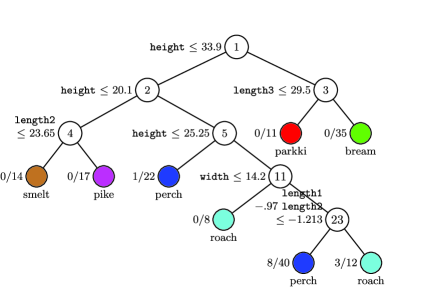
Figure 7: Tree model using the S method for the fish data. At each intermediate node, a case goes to the left child node if and only if the condition is satisfied. The predicted class and number of errors divided by sample size are printed below and to the left of each leaf node.

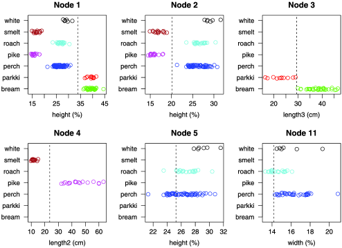
Figure 8: Plots of fish data in the intermediate nodes of the tree in Figure 7, with dashed lines marking the splits. Points are vertically jittered.

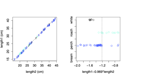
Figure 9: Plots of fish data in node 23 of the tree in Figure 7, with dashed lines marking the split. The left panel shows the data in terms of variables length1 and length2; the right panel is a jittered plot of the same data in the linear discriminant direction. The plot symbols in the left panel are the same as those in Figure 6.

Figure 7 shows the pruned tree for the fish data using this algorithm. The tree has univariate splits everywhere except at node 23, where it uses a linear split on variables length1 and length2, and misclassifies 12 observations. Figure 8 displays jittered plots of the data in the intermediate nodes with univariate splits. Figure 9 shows two views of the data in the node with the linear split; the left panel displays the data in terms of length1 and length2, and the right panel shows them in terms of the linear discriminant coordinate. Obviously, it would be impossible to show the left panel if the linear split involves more than two variables.

If linear splits are disallowed, the tree has 12 leaf nodes and misclassifies 10 observations. The CRUISE, QUEST, CTree and RPART trees have 16, 5, 7 and 6 leaf nodes and misclassify 24, 26, 28 and 21 observations, respectively. CRUISE 2V, which employs bivariate linear discriminant leaf node models, yields a tree with 5 leaf nodes and misclassifies 3.

The variable definitions in Table 2 are taken directly from the data source. If the length, width and height variables are all expressed as percentages of length3, the resulting tree has 6 leaf nodes with no linear splits and misclassifies 7 observations. Conversely, if all are expressed in cm instead of percentages, the tree has 15 leaf nodes, employs 4 linear splits and 1 interaction split, and misclassifies 17. Thus, transformations of the variables can make a difference. We note, further, that the error rates are probably biased low, because they are estimated from the same data set used to build the models. Cross-validation estimates are used to compare algorithms in Section 6.

4 Selection bias

As mentioned earlier, it is important for an algorithm to be without variable selection bias. Unbiasedness here refers to the property that the $X$ variables are selected with equal probability, when each is independent of the class variable. To show that Algorithm 3.1 is practically unbiased, we report the results of a simulation experiment with $N=500$ and six $X$ variables. The class variable takes two values with equal probabilities and is independent of the $X$ variables. We consider two scenarios. In the independence scenario, the $X$ variables are mutually independent with the following distributions:

1. [6.]

2. $X_{1}$ is categorical with $P(X_{1}=1)=P(X_{2}=2)=1/2$;

3. $X_{2}$ is categorical with $P(X_{2}=1)=1/6$, $P(X_{2}=2)=1/3$, and $P(X_{2}=3)=1/2$;

4. $X_{3}$ is categorical taking six values with equal probability;

5. $X_{4}$ is chi-squared with one degree of freedom;

6. $X_{5}$ is normal;

7. $X_{6}$ is uniform on the unit interval.

In the dependence scenario, $X_{1}$ and $X_{6}$ are independent and distributed as before, but $X_{4}$ and $X_{5}$ are bivariate normal with correlation 0.7 and $X_{2}$ and $X_{3}$ have the joint distribution shown in Table 3.

Table 3: Joint distribution of $X_{2}$ and $X_{3}$ in the dependence scenario

	$\bolds{X_{3}}$
$\bolds{X_{2}}$	1	2	3	4	5	6
1	1$/$12	1$/$12	1$/$24	1$/$24	1$/$24	1$/$24
2	1$/$24	1$/$24	1$/$12	1$/$12	1$/$24	1$/$24
3	1$/$24	1$/$24	1$/$24	1$/$24	1$/$12	1$/$12

Table 4: Number of times (out of 10,000 simulation trials) that each variable is selected to split the root node. Variables $X_{1}$, $X_{2}$ and $X_{3}$ are categorical and can only appear in a univariate split; variables $X_{4}$, $X_{5}$ and $X_{6}$ can appear in a univariate or a linear split

	Univariate splits						Linear splits
Scenario	$\bolds{X_{1}}$	$\bolds{X_{2}}$	$\bolds{X_{3}}$	$\bolds{X_{4}}$	$\bolds{X_{5}}$	$\bolds{X_{6}}$	$\bolds{X_{4}}$	$\bolds{X_{5}}$	$\bolds{X_{6}}$
Independence	1713	1656	1620	1567	1492	1533	302	310	226
Dependence	1684	1643	1601	1544	1564	1503	356	342	224

Table 5: Probabilities of variable selection for a null model estimated by simulation. The simulation standard error is 0.0037. If the method is unbiased, the probabilities should be all equal to 0.1667

	$\bolds{X_{1}}$	$\bolds{X_{2}}$	$\bolds{X_{3}}$	$\bolds{X_{4}}$	$\bolds{X_{5}}$	$\bolds{X_{6}}$
Independent	0.1713	0.1656	0.1620	0.1718	0.1647	0.1646
Dependent	0.1684	0.1643	0.1601	0.1722	0.1735	0.1615

Table 4 shows the number of times each variable is chosen over 10,000 simulation trials. Among univariate splits, there is a slightly lower probability that a noncategorical variable is selected (most likely due to discretization of the continuous variables or the Wilson–Hilferty approximation), but it is offset by the probability that such variables are selected through linear splits. Because two $X$ variables are involved in a linear split, each one is double-counted in the three columns on the right side of Table 4. Therefore, to estimate the overall selection probability for each variable, we halve these counts before adding them to the corresponding univariate split counts. The results, shown in Table 5, are all within two simulation standard errors of $1/6$ (the required value for unbiasedness).

5 Kernel and nearest-neighbor node models

So far, we have tried to make the tree structure more parsimonious and precise by controlling selection bias and improving the discriminatory power of the splits. Another way to reduce the size of the tree structure is to fit nontrivial models to the nodes. Kim and Loh cruise2v and Gama Gama04 , for example, use linear discriminant models. Although effective in improving predictive accuracy, linear discriminant models are not as flexible as nonparametric ones and may not simplify the tree structure as much. We propose to use kernel and nearest-neighbor models instead. To allow the fits to be depicted graphically, we again restrict each model to use at most two variables. Further, to save computation time, we use Algorithm 2.2 to find the split variables, skipping the linear splits. Buttrey and Karo BK02 also fit nearest-neighbor models, but they do this only after a standard classification tree is constructed. As a result, their tree structure is unchanged by model fitting. Since we fit a model to each node as the tree is grown, we should get more compact trees.

First, consider kernel discrimination, which is basically maximum likelihood with a kernel density estimate for each class in a node. If the selected $X$ variable is categorical, its class density estimate is just the sample class density function. If $X$ is noncategorical, we use a Gaussian kernel density estimate. Let $s$ and $r$ denote the standard deviation and the inter-quartile range, respectively, of a sample of observations, $x_{1},x_{2},\ldots,x_{n}$, from $X$. The kernel density estimate is $\hat{f}(x)=(nh)^{-1}\sum_{i=1}^{n}\phi\{(x-x_{i})/h\}$, where $\phi$ is the standard normal density function and $h$ is the bandwidth. The following formula, adapted from Stata stata ,

$$h=\cases{2.5\min(s,0.7413r)n^{-1/5},&\quad if $r>0$,\vspace*{2pt}\cr 2.5sn^{-1/5},&\quad otherwise,}$$ (5)

is used in the calculations reported here. This bandwidth is more than twice as wide as the asymptotically optimal value usually recommended for density estimation; Ghosh and Chaudhuri GCS06 find that the best bandwidth for discrimination is often much larger than that for density estimation. For our purposes, asymptotic formulas cannot be taken too seriously, because the node sample size decreases with splitting.

If a pair of noncategorical variables is selected, we fit a bivariate kernel density to the pair for each class. If the split is due to one categorical and one noncategorical variable, we fit a kernel density estimate to the noncategorical variable for each class and each value of the categorical variable, using an average bandwidth that depends only on the class. Averaging smoothes out the effects of small or highly unbalanced sample sizes. The details are given in the next algorithm.

Algorithm 5.1 ((Kernel models)).

Let $Y$ denote the class variable and apply Algorithm 2.2 to find one or two variables to split a node $t$:

1. [2.]

2. If the split is due to a main effect chi-squared statistic (Procedure 2.1), let $X$ be the selected variable. Fit a kernel density estimate to $X$ for each class in $t$ using bandwidth (5) with $n=N(t)$.

3. If the split is due to an interaction chi-squared statistic (Procedure 2.2), let $X_{1}$ and $X_{2}$ be the selected variables. Fit a bivariate density estimate to $(X_{1},X_{2})$ for each class in $t$ as follows:

   1. [(a)]

   2. If $X_{1}$ and $X_{2}$ are categorical, use their sample class joint density.

   3. If $X_{1}$ is categorical and $X_{2}$ is noncategorical, then for each combination of $(X_{1},Y)$ values present in $t$, find a bandwidth $h(Y,X_{1})$ using (5). Let $\bar{h}(Y)$ be the average of $h(Y,X_{1})$. For each value of $X_{1}$ and $Y$, find a kernel density estimate for $X_{2}$ with $\bar{h}(Y)$ as bandwidth.

   4. If both variables are noncategorical, fit a bivariate Gaussian kernel density estimate to each class with correlation equal to the class sample correlation and $n$ equal to the class sample size in (5).

The predicted class is the one with the largest estimated density.

We use the same idea for nearest-neighbor models. For noncategorical variables, the number of nearest neighbors, $k$, is given by the formula

$$k=\max(3,\lceil\log n\rceil),$$ (6)

where $n$ is the number of observations and $\lceil x\rceil$ denotes the smallest integer greater than or equal to $x$. We require $k$ to be no less than 3 to lessen the chance of ties. The full details are given next.

Algorithm 5.2 ((Nearest neighbor models)).

Let $\hat{Y}$ denote the predicted value of $Y$. Use Algorithm 2.2 to find one or two variables to split a node $t$:

1. [2.]

2. If the split is due to a main effect chi-squared statistic (Procedure 2.1), let $X$ be the selected variable:

   1. [(a)]

   2. If $X$ is categorical, then $\hat{Y}$ is the highest probability class among the observations in $t$ with the same $X$ value as the one to be classified.

   3. If $X$ is noncategorical, then $\hat{Y}$ is given by the $k$-nearest neighbor classifier based on $X$ with $n=N(t)$ in (6).

3. If the split is due to an interaction chi-squared statistic (Procedure 2.2), let $X_{1}$ and $X_{2}$ be the selected variables:

   1. [(a)]

   2. If both variables are categorical, then $\hat{Y}$ is the highest probability class among the observations in $t$ with the same $(X_{1},X_{2})$ values as the one to be classified.

   3. If $X_{1}$ is categorical and $X_{2}$ is noncategorical, then $\hat{Y}$ is given by the $k$-nearest neighbor classifier based on $X_{2}$ applied to the set $S$ of observations in $t$ that have the same $X_{1}$ value as the one to be classified, with $n$ being the size of $S$ in (6).

   4. If both variables are noncategorical, then $\hat{Y}$ is given by the bivariate $k$-nearest neighbor classifier based on $X_{1}$ and $X_{2}$ with the Mahalanobis distance and $n=N(t)$ in (6).

Figure 10: Three-class problem, with class 1 uniformly distributed on the circle and classes 2 and 3 each uniformly distributed on its own diagonal line.

Figure 10 shows an artificial example that is very challenging for many algorithms. There are 300 observations, with 100 from each of three classes and eight predictor variables. Class 1 is uniformly distributed on the unit circle in the $(X_{1},X_{2})$-plane. Class 2 is uniformly distributed on the line $X_{1}-X_{2}=0$, and class 3 on the line $X_{1}+X_{2}=0$, with $|X_{1}|<1$ and $|X_{2}|<1$. Variables $X_{3}$, $X_{4}$ and $X_{5}$ are uniformly distributed on the unit interval and $X_{6}$, $X_{7}$ and $X_{8}$ are categorical, each taking 21 equi-probable values. The $X$ variables are mutually independent.

QUEST with linear splits gives a 38-leaf tree that misclassifies 3 samples. CRUISE with LDA models gives a 17-leaf tree that misclassifies 10 samples. RPART, QUEST with univariate splits and our simple node method are about equal, misclassifying 85, 81 and 75 samples, respectively. C4.5 and CTree are the worst, with 134 and 200 misclassified and 84 and 1 leaf nodes, respectively. In contrast, our kernel and nearest-neighbor methods yield trees with no splits after pruning and misclassify 2 and 8 training samples, respectively.

Table 6: Algorithms and plot symbols for the comparison experiment

C45	C4.5
C2d	CRUISE with interaction detection and simple node models
C2v	CRUISE with interaction detection and linear discriminant node models
Qu	QUEST with univariate splits
Ql	QUEST with linear splits
Rp	RPART
Ct	CTree
S	Proposed method with simple node models (Algorithm 3.1)
K	Proposed method with kernel node models (Algorithm 5.1)
N	Proposed method with nearest-neighbor node models (Algorithm 5.2)

6 Comparison on forty-six datasets

The error rates discussed so far are biased low because they are computed from the same data that are used to construct the tree models. To obtain a better indication of relative predictive accuracy, we compare the algorithms listed in Table 6 on forty-two real and four artificial data sets using ten-fold cross-validation. Each data set is randomly divided into ten roughly equal parts and one-tenth is set aside in turn as a test set to estimate the predictive accuracy of the model constructed from the other nine-tenths of the data. The cross-validation estimate of error is the average of the ten estimates. Equal misclassification costs are used throughout. As elsewhere in this article, the trees are pruned to have minimum cross-validation estimate of misclassification cost. All other parameter values are set at their respective defaults.

The four artificial data sets are those in Figures 5 (int) and 10 (cl3), and the digit (led) and waveform (wav) data in cart . Sample size ranges from 97 to 45,222; number of classes from 2 to 11; number of categorical variables from 0 to 60; number of noncategorical variables from 0 to 69; and maximum number of categories among categorical variables from 0 to 41. We use the notations “S,” “K” and “N” to refer to our proposed method with simple (i.e., constant), kernel and nearest-neighbor node models, respectively. S employs linear splits, but K and N do not.

Eleven data sets have missing values. In the S, N and K algorithms, missing values in a categorical variable are assigned to their own separate “missing” category. Observations with missing values in a noncategorical split variable are always sent to the left node. If there are enough such cases, our algorithms will consider a split on missingness as one of the candidate splits. Bandwidths are computed from cases with nonmissing values in the selected variables. Kernel and nearest-neighbor model classifications are applied only to observations with nonmissing values in the selected variables. Observations with missing values in the selected variables are classified with the majority rule.

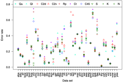
Figure 11: Error rates of algorithms by data set.

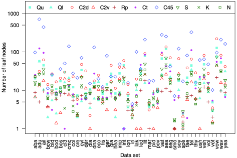
Figure 12: Numbers of leaf nodes by data set.

Figure 11 graphs the errors rates of the ten algorithms for each data set. Despite the large range of the error rates (from near 0 to about 0.7), the algorithms have very similar accuracy for about half of the data sets. The most obvious exceptions are the artificial data sets int and cl3, where our K, N and S algorithms have a superior edge; algorithms not designed to detect interactions pay a steep price here. Two other examples showing interesting patterns are the fish (fis) data used in Section 3 and the bod data set body03 , where body measurements are used to classify gender. For these two data sets, algorithms that employ LDA techniques (C2v, Ql and S) are more accurate. Ql seems to be either best or worst for a majority of the data sets.

Figure 13: Means of error rates, numbers of leaf nodes and computational times; for the top two plots, dashed lines join algorithms that do not differ significantly at the 95% simultaneous level of confidence.

Figure 12 shows the corresponding results for the sizes of the trees in terms of their numbers of leaf nodes. C45 tends to produce the largest trees, while C2v and Rp often give the shortest.

Figure 13 shows arithmetic means (over the 46 data sets) of the error rates and numbers of leaf nodes for each algorithm, with corresponding 95% Tukey simultaneous confidence intervals. The latter are obtained by fitting two-factor mixed models to the error rates and number of leaf nodes separately, using algorithm as fixed factor, data set as random factor, and their interaction as error term. S and Ct have the smallest and largest, respectively, mean error rates. The confidence intervals show that the mean error rate of Ct differs significantly from those of S, N, K and Qu; other differences are not significant. As for mean number of leaf nodes, C45 is significantly different from the others, as is Rp from C2d.

Figure 13 also shows the mean computational times, on a 2.66Ghz quad-core Linux PC with 8Gb memory. Because the algorithms are implemented in different computer languages (Rp and Ct in R, C45 in C and the others in Fortran), the results compare execution times rather than number of computer operations. Further, the mean time for Rp is dominated by two data sets each having six classes and categorical variables with many categorical levels. It is well known that the computational time of CART, upon which Rp is based, increases exponentially with the number of categorical levels when the number of classes exceeds two.

Figure 14: Mean of error rates relative to the lowest (for each data set) versus mean of tree size relative to that of the smallest tree; tree size is measured by the number of leaf nodes.

Another way to account for differences among data sets is to compare the ratio of the error rate of each algorithm to the lowest error rate among the ten algorithms within each data set. We call this ratio the “error rate relative to the lowest” for the particular algorithm and data set. The mean of these ratios for an algorithm over the data sets yields an overall measure of its relative inaccuracy. Applying the same procedure to the number of leaf nodes gives an overall measure of relative tree size for each algorithm. Figure 14 gives a plot of these two measures. The best algorithms are those in the bottom left corner of the plot: K, N, S and C2v. They are relatively most accurate and they yield relatively small trees.

7 Tree ensembles

A tree ensemble classifier uses the majority vote from a collection of tree models to predict the class of an observation. Bagging bagging96 creates the ensemble by using bootstrap samples of the training data to construct the trees. Random Forest (RF), which is based on CART and employs 500 trees, goes beyond bagging by splitting each node on a random subset of $\sqrt{K}$ variables ($K$ being the total number of variables) and not pruning the trees. Because it is practically impossible to interpret so many trees, ensemble classifiers are typically used for prediction only.

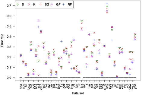
Figure 15: Single tree models (S and K) versus ensemble models (BG, GF and RF).

To see how much an ensemble can affect the predictive accuracy of the single-tree models proposed here, we use the bagging and RF ideas to create two new ensemble classifiers. The first, called bagged GUIDE (BG), is a collection of 100 pruned trees, each constructed using the S method from bootstrap samples. The second ensemble classifier, called GUIDE forest (GF), consists of 500 unpruned trees constructed by the S method without interaction and linear splits. As in RF, GF uses a random subset of $\sqrt{K}$ variables to split each node.

Figure 15 shows the error rates of BG, GF and RF compared with those of the S and K methods for each data set. The R package of Liaw and Wiener rf , which we use for RF, is not applicable if the data set has predictor variables with more than 32 categorical levels or if the test sample contains class labels that are not present among the training samples. The first condition occurs in the adu and lak data sets, which have categorical variables with 41 and 35 levels, respectively, and the second condition occurs with the eco data set, which has 8 classes and a total sample size of 336. Table 7 gives the mean error rates with these three data sets excluded. All three ensemble methods have lower means than the single-tree methods, but the differences are fairly small on average. Figure 15 shows that although RF is best for many data sets, it performs particularly poorly compared to S and K for three data sets: cl3 (Figure 10), fis (fish data in Section 3) and int (Figure 5)—data sets that have strong linear or interaction effects. GF shares the same difficulties with RF, but BG does not, because the latter allows linear and interaction splits.

Table 7: Mean error rates over the 46 data sets where RF is applicable. Differences are not statistically significant

Algorithm	S	K	BG	GF	RF
Error rate	0.228	0.231	0.212	0.212	0.206

8 Conclusion

Improving the prediction accuracy of a tree and the precision of its splits is a balancing act. On the one hand, we must refrain from searching too greedily for splits, as the resulting selection bias can cause irrelevant variables to be selected. On the other hand, we should search hard enough to avoid overlooking good splits hidden behind interactions or linear relationships. We solve this problem by using three groups of significance tests, with increasing complexity of effects and decreasing order of priority. The first group of tests for main effects is always carried out. The second group, which tests for interactions, is performed only if no main effect test is significant. The third group, which tests for linear structure, is performed only if no test in the first two groups is significant. A Bonferroni correction controls the significance level of each group. In addition, if an interaction test is significant, the split is found by a two-level search on the pair of interacting variables.

If greater reduction in the size of the tree structure is desired, we can fit a kernel or a nearest-neighbor model to each node. Owing to the flexibility of these models, we dispense with linear splits in such situations. We showed by an example that when there are weak main effects but strong two-factor interaction effects, classification trees constructed with these models can achieve substantial gains in accuracy and tree compactness. They require more computation than trees with simple node models, but the empirical evidence indicates that their prediction accuracy remains high even for ordinary data sets.

We also investigated the effect of tree ensembles on predictive accuracy. Although Random Forest quite often yields higher accuracy than the single-tree models S and K, the average increase is only about 10% for the 43 data sets in the study. Much depends on the complexity of the data. If there are strong interaction or linear effects, the single-tree algorithms proposed here can be substantially more accurate than Random Forest. Further, the choice of the single-tree algorithm used in the ensemble matters.

All the proposed algorithms are implemented in version 8 of GUIDE, which may be obtained from www.stat.wisc.edu/~loh/guide.html for the Linux, Macintosh and Windows operating systems.

Appendix

Procedure .1.

Split set selection for a categorical variable $X$. Let $\{a_{1},a_{2},\ldots,a_{n}\}$ be the set of distinct values of $X$ in node $t$:

1. [3.]

2. If $J=2$ or $n\leq 11$, search all subsets $S$ to find a split of the form $t_{L}=\{X\in S\}$ that minimizes (2).

3. Else if $J\leq 11$ and $n>20$, for each $i=1,2,\ldots,n$, let $j_{i}$ be the class that minimizes the misclassification cost for the observations in $t\cap\{X=a_{i}\}$. Define the new categorical variable $X^{\prime}=\sum_{i}j_{i}I(X=a_{i})$ and search all subsets $S^{\prime}$ to find a split of the form $\{X^{\prime}\in S^{\prime}\}$ that minimizes (2). Re-express the selected split in terms of $X$ as $t_{L}=\{X\in S\}$.

4. Else use LDA as follows:

   1. [(c)]

   2. Convert $X$ into a vector of dummy variables $(u_{1},u_{2},\ldots,u_{n})$, where $u_{i}=1$ if $X=a_{i}$ and $u_{i}=0$ otherwise.

   3. Obtain the covariance matrix of the $u$-vectors and find the eigenvectors associated with the positive eigenvalues. Project the $u$-vectors onto the space spanned by these eigenvectors.

   4. Apply LDA to the projected $u$-vectors to find the largest discriminant coordinate $v=\sum_{i}c_{i}u_{i}$.

   5. Let $v_{(1)}<v_{(2)}<\cdots$ denote the (at most $n$) sorted $v$-values.

   6. Find the split $t_{L}=\{v\leq v_{(m)}\}$ that minimizes (2).

   7. Re-express the split as $t_{L}=\{X\in S\}$.

Procedure .2.

Split selection between two noncategorical variables $X_{1}$ and $X_{2}$. Let $S_{k}$ ($k=1,2$) be defined as in (4):

1. [3.]

2. Split $t$ first on $X_{1}$ and then on $X_{2}$ as follows. Given numbers $c$, $d$ and $e$, let $t_{L}=\{X_{1}\leq c\}$, $t_{R}=\{X_{1}>c\}$, $t_{\mathit{LL}}=t_{L}\cap\{X_{2}\leq d\}$, $t_{\mathit{LR}}=t_{L}\cap\{X_{2}>d\}$, $t_{\mathit{RL}}=t_{R}\cap\{X_{2}\leq e\}$, and $t_{\mathit{RR}}=t_{R}\cap\{X_{2}>e\}$. Search over all $c\in S_{1}$ and $d,e\in S_{2}$ to find the best $c=c_{1}$ that minimizes (3).

3. Exchange the roles of $X_{1}$ and $X_{2}$ in the preceding step to find the best split $\{X_{2}\leq c_{2}\}$ with $c_{2}\in S_{2}$.

4. If the minimum value of (3) from the split $\{X_{1}\leq c_{1}\}$ is less than that from $\{X_{2}\leq c_{2}\}$, select the former. Otherwise, select the latter.

Procedure .3.

Split selection between noncategorical $X_{1}$ and categorical $X_{2}$:

1. [3.]

2. First find a split of $t$ on $X_{1}$ as follows. Let $t_{L}=\{X_{1}\leq c\}$ and $t_{R}=\{X_{1}>c\}$, where $c\in S_{1}$ and $S_{1}$ is defined in (4):

   1. [(a)]

   2. Consider the observations in $t_{L}$. If $J>2$, form two superclasses, with one containing the class that minimizes the misclassification cost in $t_{L}$ and the other containing the rest. Use Theorem 2.1 to obtain an ordering $a_{1}\prec a_{2}\prec\cdots$ of the values of $X_{2}$. Define $A_{i}=\{a_{1},a_{2},\ldots,a_{i}\}$, $t_{\mathit{LL}}=t_{L}\cap\{X_{2}\in A_{i}\}$, and $t_{\mathit{LR}}=t_{L}\cap\{X_{2}\notin A_{i}\}$ for $i=1,2,\ldots.$

   3. Repeat the preceding step on the observations in $t_{R}$ to obtain an ordering $b_{1}\prec b_{2}\prec\cdots$ of the values of $X_{2}$. Define $B_{j}=\{b_{1},b_{2},\ldots,b_{j}\}$, $t_{\mathit{RL}}=t_{R}\cap\{X_{2}\in B_{j}\}$, and $t_{\mathit{RR}}=t_{R}\cap\{X_{2}\notin B_{j}\}$ for $j=1,2,\ldots.$

   4. Let $\delta_{1}$ be the minimum value of (3) over $\{A_{i}\}$, $\{B_{j}\}$, and $c\in S_{1}$. Let $c^{*}$ be the minimizing value of $c$.

3. Find the following two splits of $t$ on $X_{2}$:

   1. [(a)]

   2. Order the values of $X_{2}$ in the set $\{X_{1}\leq c^{*}\}$ according to step 1 above and use them to generate splits of the form $t_{L}=\{X_{2}\in U_{i}\}$ and $t_{R}=\{X_{2}\notin U_{i}\}$, $i=1,2,\ldots.$ For each $i$, find the best splits of $t_{L}$ and $t_{R}$ on $X_{1}$ into $t_{\mathit{LL}}$, $t_{\mathit{LR}}$ and $t_{\mathit{RL}}$, $t_{\mathit{RR}}$, respectively. Let $\delta_{2}$ be the minimum value of (3), attained at $t_{L}=\{X_{2}\in U\}$, say.

   3. Repeat the preceding step on the observations in $\{X_{1}>c^{*}\}$ to get the split $t_{L}=\{X_{2}\in V\}$, say, with minimizing value $\delta_{3}$.

4. If $\delta_{1}\leq\min(\delta_{2},\delta_{3})$, split $t$ with $\{X_{1}\leq c^{*}\}$. Otherwise, select $\{X_{2}\in U\}$ if $\delta_{2}\leq\delta_{3}$, and $\{X_{2}\in V\}$ if $\delta_{2}>\delta_{3}$.

Procedure .4.

Split selection between categorical variables $X_{1}$ and $X_{2}$:

1. [3.]

2. Given $U$, $V$ and $W$, let $t_{L}=\{X_{1}\in U\}$, $t_{R}=\{X_{1}\notin U\}$, $t_{\mathit{LL}}=t_{L}\cap\{X_{2}\in V\}$, $t_{\mathit{LR}}=t_{L}\cap\{X_{2}\notin V\}$, $t_{\mathit{RL}}=t_{R}\cap\{X_{2}\in W\}$, and $t_{\mathit{RR}}=t_{R}\cap\{X_{2}\notin W\}$. Let $k_{1}$ be the number of distinct values of $X_{1}$:

   1. [(a)]

   2. If $J=2$, search over all sets $U$, $V$ and $W$.

   3. If $J>2$ and $k_{1}\leq 5$, search over all sets $U$ but restrict the sets $V$ and $W$ as follows. Let $j_{0}$ be the class that minimizes the misclassification cost in $t$ and create two superclasses, with one containing $j_{0}$ and the other containing the rest. Use Theorem 2.1 on the two superclasses to induce an ordering of the $X_{2}$-values and then search for $V$ and $W$ using the ordered values.

   4. If $J>2$ and $k_{1}>5$, use the method in the preceding step to restrict the search on $U$, $V$ and $W$.

   Let $\delta_{1}$ be the smallest searched value of (3), and let it be attained at $U=U^{\prime}$.

3. Repeat step 1 with the roles of $X_{1}$ and $X_{2}$ reversed and let $\delta_{2}$ be the minimum value of (3), attained with $t_{L}=\{X_{2}\in V^{\prime}\}$.

4. Split $t$ with $\{X_{1}\in U^{\prime}\}$ if $\delta_{1}\leq\delta_{2}$; otherwise, split with $\{X_{2}\in V^{\prime}\}$.

References

- (1) Amasyali, M. F. and Ersoy, O. (2008). CLINE: A new decision-tree family. IEEE Transactions on Neural Networks 19 356–363.
- (2) Atkinson, E. J. and Therneau, T. M. (2000). An introduction to recursive partitioning using the RPART routines. Technical report 61, Biostatistic Section, Mayo Clinic, Rochester, NY.
- (3) Breiman, L. (1996). Bagging predictors. Mach. Learn. 24 123–140. \MR1425957
- (4) Breiman, L. (2001). Random forests. Mach. Learn. 45 5–32.
- (5) Breiman, L., Friedman, J. H., Olshen, R. A. and Stone, C. J. (1984). Classification and Regression Trees. Wadsworth, Belmont. \MR0726392
- (6) Buttrey, S. E. and Karo, C. (2002). Using k-nearest-neighbor classification in the leaves of a tree. Comput. Statist. Data Anal. 40 27–37. \MR1930465
- (7) Cantu-Paz, E. and Kamath, C. (2003). Inducing oblique decision trees with evolutionary algorithms. IEEE Transactions on Evolutionary Computation 7 54–68.
- (8) Clark, V. (2004). SAS/STAT 9.1 User’s Guide. SAS Publishing, Cary, NC.
- (9) Doyle, P. (1973). The use of Automatic Interaction Detector and similar search procedures. Operational Research Quarterly 24 465–467. \MR0324682
- (10) Fan, G. (2008). Kernel-induced classification trees and random forests. Manuscript.
- (11) Gama, J. (2004). Functional trees. Mach. Learn. 55 219–250.
- (12) Ghosh, A. K., Chaudhuri, P. and Sengupta, D. (2006). Classification using kernel density estimates: Multiscale analysis and visualization. Technometrics 48 120–132. \MR2236534
- (13) Heinz, G., Peterson, L. J., Johnson, R. W. and Kerk, C. J. (2003). Exploring relationships in body dimensions. Journal of Statistics Education 11. Available at www.amstat.org/publications/jse/v11n2/datasets.heinz.html.
- (14) Hosmer, D. W. and Lemeshow, S. (2000). Applied Logistic Regression, 2nd ed. Wiley, New York.
- (15) Hothorn, T., Hornik, K. and Zeileis, A. (2006). Unbiased recursive partitioning: A conditional inference framework. J. Comput. Graph. Statist. 15 651–674. \MR2291267
- (16) Kim, H. and Loh, W.-Y. (2001). Classification trees with unbiased multiway splits. J. Amer. Statist. Assoc. 96 589–604. \MR1946427
- (17) Kim, H. and Loh, W.-Y. (2003). Classification trees with bivariate linear discriminant node models. J. Comput. Graph. Statist. 12 512–530. \MR2002633
- (18) Lee, T.-H. and Shih, Y.-S. (2006). Unbiased variable selection for classification trees with multivariate responses. Comput. Statist. Data Anal. 51 659–667. \MR2297477
- (19) Li, X. B., Sweigart, J. R., Teng, J. T. C., Donohue, J. M., Thombs, L. A. and Wang, S. M. (2003). Multivariate decision trees using linear discriminants and tabu search. IEEE Transactions on Systems Man and Cybernetics Part A–Systems and Humans 33 194–205.
- (20) Li, Y. H., Dong, M. and Kothari, R. (2005). Classifiability-based omnivariate decision trees. IEEE Transactions on Neural Networks 16 1547–1560.
- (21) Liaw, A. and Wiener, M. (2002). Classification and regression by randomforest. R News 2 18–22. Available at http://CRAN.R-project.org/doc/Rnews/.
- (22) Lim, T.-S., Loh, W.-Y. and Shih, Y.-S. (2000). A comparison of prediction accuracy, complexity, and training time of thirty-three old and new classification algorithms. Mach. Learn. J. 40 203–228.
- (23) Loh, W.-Y. (2002). Regression trees with unbiased variable selection and interaction detection. Statist. Sinica 12 361–386. \MR1902715
- (24) Loh, W.-Y. and Shih, Y.-S. (1997). Split selection methods for classification trees. Statist. Sinica 7 815–840. \MR1488644
- (25) Loh, W.-Y. and Vanichsetakul, N. (1988). Tree-structured classification via generalized discriminant analysis (with discussion). J. Amer. Statist. Assoc. 83 715–728. \MR0963799
- (26) McCullagh, P. and Nelder, J. A. (1989). Generalized Linear Models, 2nd ed. Chapman and Hall, London. \MR0727836
- (27) Morgan, J. N. and Messenger, R. C. (1973). THAID: A sequential analysis program for the analysis of nominal scale dependent variables. Technical report, Institute for Social Research, Univ. Michigan, Ann Arbor.
- (28) Morgan, J. N. and Sonquist, J. A. (1963). Problems in the analysis of survey data, and a proposal. J. Amer. Statist. Assoc. 58 415–434.
- (29) Noh, H. G., Song, M. S. and Park, S. H. (2004). An unbiased method for constructing multilabel classification trees. Comput. Statist. Data Anal. 47 149–164. \MR2087934
- (30) Perlich, C., Provost, F. and Simonoff, J. S. (2003). Tree induction vs. logistic regression: A learning-curve analysis. J. Mach. Learn. Res. 4 211–255. \MR2050883
- (31) Quinlan, J. R. (1993). C4.5: Programs for Machine Learning. Morgan Kaufmann, San Mateo.
- (32) StataCorp. (2003). Stata Statistical Software: Release 8.0. Stata Corporation, College Station, TX.
- (33) Strobl, C., Boulesteix, A.-L. and Augustin, T. (2007). Unbiased split selection for classification trees based on the Gini index. Comput. Statist. Data Anal. 52 483–501. \MR2409997
- (34) Wilson, E. B. and Hilferty, M. M. (1931). The distribution of chi-square. Proc. Nat. Acad. Sci. USA 17 684–688.
- (35) Witten, I. H. and Frank, E. (2005). Data Mining: Practical Machine Learning Tools and Techniques, 2nd ed. Morgan Kaufmann, San Fransico, CA.
- (36) Yildlz, O. T. and Alpaydin, E. (2005). Linear discriminant trees. International Journal of Pattern Recognition and Artificial Intelligence 19 323–353.