Assumptions of IV Methods for Observational Epidemiology

Abstract

Instrumental variable (IV) methods are becoming increasingly popular as they seem to offer the only viable way to overcome the problem of unobserved confounding in observational studies. However, some attention has to be paid to the details, as not all such methods target the same causal parameters and some rely on more restrictive parametric assumptions than others. We therefore discuss and contrast the most common IV approaches with relevance to typical applications in observational epidemiology. Further, we illustrate and compare the asymptotic bias of these IV estimators when underlying assumptions are violated in a numerical study. One of our conclusions is that all IV methods encounter problems in the presence of effect modification by unobserved confounders. Since this can never be ruled out for sure, we recommend that practical applications of IV estimators be accompanied routinely by a sensitivity analysis.

, and

1 Introduction

Inferring causation in observational studies is problematic, as observed associations can often be due to other than causal explanations, confounding being of special concern. Randomized controlled trials (RCTs), rendering all other explanations unlikely by design, are the accepted standard approach to causal inference. However, we are here interested in epidemiological applications where it is not always possible nor desirable to carry out RCTs. For example, it would be unethical or impractical to randomly allocate individuals to exposures such as smoking, alcohol consumption, and complex nutritional or exercise regimes. Furthermore, the cohort of a trial might not be representative of the target population for which health interventions are required DaveySmithEbrahim2003 , Lawloral2008a . The standard approach to causal inference from observational data is to assume that there is no unobserved confounding, that is, that a sufficient set of covariates has been measured. This is often implausible and has produced misleading results in the past, for example, regarding the effects of hormone replacement therapy LawlorDaveySmith2006 , HRTRCT2002 .

Methods exploiting instrumental variables provide an alternative solution. Suppose we are interested in the causal effect of some exposure (e.g., cholesterol) on disease (e.g., coronary heart disease), and believe that important confounding factors are likely but unobservable, perhaps because they are not fully understood. Loosely speaking, an instrumental variable (IV) is a third (observable) variable that is predictive of exposure, but has no direct effect on the disease and is independent of the unobserved confounders. In general, it is difficult to find a variable that can be justified as a suitable IV for any particular problem. For randomized trials with partial compliance, where the effect of the actual treatment taken is of interest, the natural IV is the randomization to treatment Greenland2000 ; but, of course, this is not an option when considering exposures that cannot be randomized as mentioned earlier. Examples in epidemiological contexts are the physician’s prescription preference as an IV to assess drug effects Brookhart2007 , Rassenal2009c , cigarette price to assess the effects of smoking LeighSchembri2004 or genetic variants that are associated with exposures of interest DaveySmithEbrahim2003 , Katan1986 , Lawloral2008a . The latter has become known as Mendelian randomization and, due to the fact that it is currently generating a lot of interest in the epidemiological literature, will serve as illustration throughout (see Section 2).

Relying only on their defining properties, IVs canbe used to test for or bound the causal effect Angristal1996 , BalkePearl1994 , DidelezSheehan2007b , Greenland2000 , HernanRobins2006 , Robins1994 . However, identification and hence point estimates of the causal effect are only obtainable under additional parametric and distributional assumptions. Linear structural equation models, popular in the econometrics literature Wooldridge1 , Zohoori1 , are a well-studied model class that allows identification. Generalizations to nonlinear structural equationsbased on log-linear or probit modeling, for example Mullahy1997 , WindmeijerSantosSilva1997 , are also available (see overview ClarkeWindmeijer2009 ). Inspired by the simplicity of the linear case, where the IV estimator is given as the ratio of the coefficients from the regressions of outcome on IV and exposure on IV, alternative methods have been put forward replacing these two linear regressions by nonlinear ones. One such example which is popular in Mendelian randomization studies with binary outcomes is what we will call the “Wald-type” estimator. This combines odds ratios or risk ratios for the genotype-outcome relationship with the mean difference in exposure given the genotype Casasal2005 , Casasal2006 , DaveySmithEbrahim2003 , Keavneyal2006 , Lawloral2008b , Thompsonal2005 .

An important consideration when using IV methods is the target of inference, that is, the precise definition of the causal parameter of interest. In our experience, epidemiologists are mostly interested in the population causal effect, that is, a comparative measure of subjecting everyone in a given population to exposure as opposed to no exposure, as would ideally be obtained in an RCT. However, some prominent IV methods target causal effects within specific subgroups. These are the effect of treatment on the compliers Angristal1996 , ImbensAngrist1994 , or the effect of treatment on the treated HernanRobins2006 , Robins1989 , RobinsRotnitzky2004 , VansteelandtGoetghebeur2003 . The complier causal effect is motivated by RCTs with partial compliance and contrasts the effect of treatment versus nontreatment for those individuals who follow their assignment whatever it is. In our view, the interpretation of this causal parameter is very much bound to the randomization scenario and we will therefore not consider it any further. The effect of “treatment on the treated” can be translated as the “effect of exposure on the exposed” in an epidemiological context and describes the effect of preventing those who would normally be exposed from becoming exposed. This particular subgroup effect is explicitly modeled by structural mean models (SMMs) HernanRobins2006 .

In this paper we compare the above approaches with regard to their use in observational epidemiology and focus on issues that have recently arisen, for example, in Mendelian randomization applications, to make the discussion concrete. We formally consider the targeted causal parameters and the underlying modeling assumptions of IV methods. We argue that their assumptions should be made explicit so that those most plausible for a given problem can be chosen. As models are never expected to be exactly true in practice, we complement the theoretical comparison by a numerical study of the possible bias under violations of the assumptions. The outline of the paper is as follows. In Section 2 we begin by presenting the basic idea of IVs with the example of Mendelian randomization as recently applied to investigate the effects of alcohol consumption. We then introduce the main concepts of causal inference in Section 3, a central issue being the different notions of causal effect parameters. Section 3.2 gives the core conditions characterizing an instrumental variable. In Section 4 we present the IV models that we will consider, and provide general indications of how they interrelate. Section 5 investigates the performance in terms of relative asymptotic bias of these methods in a numerical study where we focus on the particular case where all variables are binary in order to facilitate exact evaluation of the relevant quantities. We conclude with a discussion of the implications, both for epidemiological applications and more generally.

2 Using a Genetic Variant as an IV

We will relate to Mendelian randomization throughout the paper as a concrete application of an IV approach in observational epidemiology and outline the basic idea here using an example taken from Chen et al. Chenal2008 . Further details, including history and nomenclature, are provided in a recent review Davey2007 .

Alcohol consumption has been found in observational studies to have a positive effect on coronary heart disease (CHD) and negative effects on liver cirrhosis, some cancers and mental health problems. These findings, however, are strongly suspected to be confounded by factors like diet, lifestyle and socioeconomic factors. Thus, in order to inform public health recommendations on alcohol intake, for example, it is important to verify which, if any, of these observed associations is in fact causal for the relevant health outcome.

The connection between the ALDH2 gene and alcohol consumption is well established and understood Bosron1986 , Enomoto1991 , George4 , Yoshida1984 . The ALDH2*2 variant is associated with an accumulation of acetaldehyde and hence with unpleasant symptoms after drinking alcohol. Carriers of this variant tend to limit their alcohol consumption regardless of their other lifestyle behaviors. Since genes are randomly assigned during meiosis, ALDH2*2 carriers should not differ systematically from carriers of the ALDH2*1 allele in any other respect. In particular, there should be no association between the variant and the unobserved confounders of the various relationships between alcohol consumption and above health outcomes. The plausibility of this assumption is strengthened by the fact that there is no evidence of ALDH2 association with typical known epidemiological confounders such as age, smoking, BMI, cholesterol, etc. DaveySmithal2007 . The possibility that ALDH2 affects the particular disease of interest by any route other than through alcohol consumption can also be excluded from the known functionality of the gene. Thus, for any specific disease, we should observe that there are more *1*1 and *1*2 than *2*2 genotypes among the affected individuals if alcohol consumption is really causal for that disease. The meta-analysis by Chen et al. Chenal2008 , based mainly on studies in Japanese populations, shows that blood pressure and risk of hypertension is higher for *1*1 than for *2*2 homozygotes, and is also higher for heterozygotes (*1*2) than for the *2*2 homozygotes. As the heterozygotes tend to be moderate drinkers due to less pronounced adverse symptoms, the study concludes that even moderate alcohol consumption is “harmful” for blood pressure.

The example shows how ALDH2 can be used as an IV to provide evidence for a causal effect of the exposure by establishing that the disease and the IV are associated: the risks of high blood pressure and hypertension are significantly different between the different genotypes. As ALDH2 is assumed to have no direct effect on blood pressure or hypertension other than through alcohol consumption, the observed associations must be due to an effect of alcohol consumption on blood pressure and hypertension. Since the above assumptions define an IV, this reasoning only holds if we can be fairly confident that ALDH2 is a valid IV. Hence, only well-understood genotypes can be used as IVs. Note, this does not yet provide a point estimate of the causal effect of alcohol consumption on hypertension: it is merely evidence that there is such an effect.

The number of applications of Mendelian randomization is growing rapidly Casasal2005 , DaveySmithal2005 , George5 , DaveySmithal2005c , George4 , Lewis2 , Minellial2004 , Thompsonal2005 ; a brief overview of some recent studies is given in Sheehan et al. Sheehanal2008 . Note that even when a genetic variant can be found that is associated with the exposure of interest, it does not automatically qualify as an IV. Problems could occur when there are different subpopulations with different allele frequencies and different prevalences of disease, for instance, CardonPalmer2003 . Finding a suitable genetic instrument is thus a challenge as discussed in detail in several papers DaveySmithEbrahim2003 , DidelezSheehan2007b , DidelezSheehan2007 , Lawloral2008a , Nitschal2006 , ThomasConti2004 .

3 Causal Inference

Epidemiologists are concerned with identifying the causal effect of an exposure $X$ on a disease $Y$, typically with the view to informing public health interventions. We therefore regard causal inference to be about the effect of intervening in, or manipulating, a given system as is implicit in many approaches to causal inference Dawid2002 , DidelezSheehan2007 , Hernan2004 , Lauritzen2000 , Pearl1995 , Robins1989 , Rubin1974 , Rubin1978 .

It is useful to introduce notation to represent intervention. Pearl Pearl2000 uses the do operator to distinguish between conditioning on an intervention in $X$, $P(Y|\operatorname{do}(X=x))$, and the usual conditioning on observing $X$, $P(Y|X=x)$. The former reflects how the distribution of $Y$ should be modified when $X$ has been forced to the value $x$ by some external intervention, whereas the latter reflects how the distribution of $Y$ should be modified when $X=x$ is simply observed. The different conditions, observation versus intervention, reflect the common wisdom correlation is not causation. Note that we often write $\operatorname{do}(x)$ for $\operatorname{do}(X=x)$.

Another formal approach is based on counterfactual (potential outcome) variables Hernan2004 , Rubin1974 , Rubin1978 . Here $Y(x_{1})$ denotes the value that the outcome $Y$ would have if the variable $X$ were set to the value $x_{1}$, whereas $Y(x_{2})$ is the outcome if the same variable $X$ were set to the value $x_{2}$. The variables $Y(x_{1})$ and $Y(x_{2})$ are counterfactual because they can never both be observed together, so when one is fact, the other one is, of necessity, contrary to fact. The notion of intervention also underlies the counterfactual approach Hernan2004 , Robins2 , Rubin1974 , Rubin1978 . Both approaches define a formal language for causality and provide specific mathematical notation for representing interventions that we might be interested in. Hence, they force us to be clear and explicit about any assumptions underlying a given method of causal inference.

3.1 Causal Parameters

Causal effect parameters are typically functions of the distribution of $Y$ under different interventions in $X$. The most popular is the average causal effect (ACE) defined as the expected difference in $Y$ under two different settings of $X$:

$$\operatorname{ACE}(x_{1},x_{2}):=E(Y|\operatorname{do}(x_{2}))-E(Y|\operatorname{do}(x_{1})),$$

where $x_{1}$ is typically some baseline value. The ACE is a natural choice of causal parameter when the effect of $X$ is suspected to be linear on $Y$. When $Y$ is nonnegative or binary, in contrast, it is more common to use a multiplicative measure like the causal relative risk (CRR) defined as

$$\operatorname{CRR}(x_{1},x_{2}):=\frac{E(Y|\operatorname{do}(x_{2}))}{E(Y|\operatorname{do}(x_{1}))},$$ (1)

or, for binary $Y$, the causal odds ratio (COR) given by

$$\operatorname{COR}(x_{1},x_{2}):=\frac{P(Y=1|\operatorname{do}(x_{2}))P(Y=0|\operatorname{do}(x_{1}))}{P(Y=0|\operatorname{do}(x_{2}))P(Y=1|\operatorname{do}(x_{1}))}.$$

Note that the odds ratio is mainly used in case-control studies to approximate the relative risk in the case of a rare disease.

All these causal parameters are population parameters, that is, they compare setting $X=x_{1}$ with setting $X=x_{2}$ for the whole population of interest. They are what is measured in a comparison of the active and control groups in a controlled randomized experiment when all subjects comply with their treatment assignment. In some situations, we may be more interested in the causal effect within a subset of the population, that is, conditional on a specific value of some observed covariates. For example, we might want to know the average causal effect of male alcohol consumption on oesophageal cancer risk. The above causal parameters can easily be adapted by conditioning on covariates provided these are prior to exposure. We will not consider this further in the present paper.

However, one particular causal subgroup effect, or local causal effect, is very relevant in the epidemiological literature. This is the effect of exposure on the exposed group Greenland2000 , Robins1989 , Robins1994 , or the effect of treatment received as it is known in the context of clinical trials (cf. Elwood2007 , e.g.). For example, we might be interested in the effect of reducing alcohol consumption for those individuals who would normally tend to have high alcohol consumption, but not in the question of increasing alcohol consumption for those who normally do not drink much. This does not quite correspond to conditioning on observed covariates, as what the subjects “would normally” be exposed to in the future is not usually observable. However, it can be assumed that if no intervention takes place, alcohol consumption will remain high for those individuals with existing high consumption. In counterfactual notation the corresponding local causal relative risk, LCRR, for instance, is given by

$$\operatorname{LCRR}:=\frac{E(Y(x)|X=x)}{E(Y(0)|X=x)},$$ (2)

where $Y(x)$ is the value of the outcome if an individual’s alcohol consumption is set to be $x$ and $Y(0)$ is the counterfactual outcome if it is set to be at a baseline level, while conditioning on $X=x$ means that the “natural” alcohol consumption is $x$. Note that given $X=x$, we actually observe $Y=Y(x)$, so that the numerator of (2) is equal to $E(Y|X=x)$. This type of causal parameter can also be expressed with the $do$-notation, but we need to distinguish between the “natural” value of exposure $X$ and the one that it is set to by intervention $\tilde{X}$. When no intervention takes place, these two are identical, that is, $X\equiv\tilde{X}$. However, when an intervention takes place, it is assumed that $\tilde{X}$ “overrules” $X$ so that $Y$ causally depends on $\tilde{X}$ while being still associated with $X$ due to the fact that $X$ is informative for the unobserved confounding that also predicts $Y$. The above can then be translated to

$$\operatorname{LCRR}:=\frac{E(Y|X=x,\operatorname{do}(\tilde{X}=x))}{E(Y|X=x,\operatorname{do}(\tilde{X}=0))}.$$ (3)

See Robins, VanderWeele and Richardson Robinsal2006 and Geneletti and Dawid GenelettiDawid2007 for more details on how to interpret this local causal effect without counterfactual notation. Local versions of the ACE and COR can easily be defined analogously to the above LCRR. Note that the term “local” causal effect in the IV literature is most commonly used for the effect of treatment on the “compliers” in an RCT Angristal1996 , Greenland2000 , ImbensAngrist1994 , which we are not dealing with here and which is different from (3).

One further causal parameter that is sometimes considered is the individual causal effect which is expressed with potential outcomes as $Y^{i}(x_{2})-Y^{i}(x_{1})$. It is the difference between the potential outcomes for a specific individual $i$. Assumptions under which the individual causal effect can be identified are inherently untestable Dawid2000 , but may be justified given specific subject matter background knowledge.

Finally, we want to emphasize that a population parameter like CRR in (1) will be different from a conditional or local parameter LCRR in (2) or from an individual causal effect when the effect of exposure is different in different subgroups or individuals, that is, under heterogeneity or effect modification. For instance, those who naturally have a high alcohol consumption are likely to be different in many other relevant but unobservable respects than those who have a naturally low alcohol consumption and, therefore, the effect of changing that level should be different in these two groups. In particular, there may be no overall effect in the population (i.e., $\operatorname{CRR}=1$) if negative and positive effects in subgroups (or individuals) cancel each other out. In such a situation, an estimator that targets the CRR will be biased for the LCRR and vice versa. We reiterate that the accepted gold standard RCT randomizing individuals to either $x_{1}$ or $x_{2}$ always targets a population causal effect.

3.2 Instrumental Variables

The standard approach to estimating a causal parameter from observational data is to assume that a sufficient set of observed confounders is available for which we then adjust Dawid2002 , Greenlandal1999b , Lauritzen2000 , Pearl2000 , Rubin1974 . When there is reason to suspect additional unobserved confounding, the causal effect cannot typically be obtained in this way. In this situation, IV methods permit a different way of performing causal inference by exploiting the additional information provided by the instrumental variable.

Recall that we denote the exposure of interest (intermediate phenotype or modifiable risk factor) by $X$ and the outcome (disease) by $Y$. Furthermore, we let $G$ be the instrument (e.g., genotype in a Mendelian randomization study) and $U$ an unobserved variable (or, more realistically, a set of unobserved variables) that will represent the confounding between $X$ and $Y$. The properties that define an IV are expressed in terms of conditional independence statements where $A\perp\!\!\!\!\perp B|C$ means $A$ is independent of $B$ given $C$. The core conditions are the following: [1.]

$G\perp\!\!\!\!\perp U$, that is, $G$ must be (marginally) independent of the confounding between $X$ and $Y$;

$G\not\perp\!\!\!\!\perp X$, that is, $G$ must not be (marginally) independent of $X$;

$G\perp\!\!\!\!\perp Y|(X,U)$, that is, conditionally on $X$ and the confounder $U$, the instrument and the response are independent.

These properties can, to a limited extent, be tested from the observable data (i.e., without measurements on $U$) when $G,X,Y$ are all categorical. This is because they impose certain inequality constraints on the joint distribution $p(y,x,g)$ (see Pearl1995b , Pearl2000 for details). Analogous constraints can also be obtained for situations where joint observation of $(G,X,Y)$ is not possible, but separate observations on $(G,X)$ and $(G,Y)$ are available from different studies Ramsahai2007 , for instance, as is often the case for Mendelian randomization applications. Furthermore, Ramsahai Ramsahaiphd develops a statistical test for violation of these inequality constraints that properly accounts for the sampling variability in the estimated probabilities. When the data are categorical, these inequalities should always be verified in order to detect “gross” violations of the above core conditions. However, it should be kept in mind that distributions $p(y,x,g,u)$ will exist which violate the core conditions but may have marginals $p(y,x,g)$ that still satisfy these inequalities. We are not aware of analogous inequality constraints that could be checked when $X$ is continuous (but see Bonet2001 for the case where instrument or outcome are continuous). Categorizing continuous variables is not advisable, as it is possible that the continuous variables satisfy the above core conditions, while their discrete versions do not. Hence, since a test of the inequalities can only falsify the core assumptions but never confirm them, and since it cannot be carried out when the exposure is continuous, it is crucial to always justify the core conditions on the basis of subject matter or other relevant background knowledge.

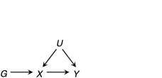
Figure 1: The DAG representing the core conditions required for $G$ to be an instrument.

A shorthand way of encoding conditional independence restrictions is via graphical models Cowellal1999 . The directed acyclic graph (DAG) in Figure 1 is the unique representation of the above core conditions. Furthermore, this graph is equivalent to a factorization of the joint density on $(Y,X,U,G)$ in the following way:

$$p(y,x,u,g)=p(y|u,x)p(x|u,g)p(u)p(g).$$ (4)

While this describes how the variables behave “naturally,” we have to specify our assumptions about how an intervention in $X$ operates on the system. This takes the form of an additional structural assumption which states that intervening in $X$ does not affect the distributions of any other factors in (4) besides the conditional distribution of $X$. Under intervention on $X$, the joint distribution of (4) thus becomes

$$p(y,u,g,x|\operatorname{do}(x_{0}))$$

(5)

$$\quad=p(y|u,x_{0})I(x=x_{0})p(u)p(g),$$

where $I(\cdot)$ is the indicator function. The corresponding DAG in Figure 2 graphically shows the conditional independence relationships among $Y,G$ and $U$ for the core conditions and an intervention on $X$. One immediate implication is that $G\perp\!\!\!\!\perp Y|\operatorname{do}(X)$, which is also known as the exclusion restriction condition in the IV literature, where it is typically expressed with potential outcomes as $G\perp\!\!\!\!\perp Y(x)$ Angristal1996 , ImbensAngrist1994 .

Figure 2: The DAG representing the core conditions under intervention in $X$.

Taking this a step further, we can also express the IV assumptions when the effect of exposure on the exposed individuals is of interest. Using the notation introduced in Section 3.1, let $X$ denote the “natural” exposure level, while $\tilde{X}$ denotes the exposure that is set by an intervention. When there is no intervention, they are identical and (4) is valid. Under intervention, $\tilde{X}$ overrules the “natural” $X$ with respect to the conditional distribution of $Y$ and we obtain the joint distribution under intervention

$$p\bigl{(}y,u,g,X=x|\operatorname{do}(\tilde{X}=x_{0})\bigr{)}$$

$$\quad=p(y|u,x_{0})p(X=x|u,g)p(u)p(g),$$

which can again be represented graphically with a DAG as in Figure 3 GenelettiDawid2007 , Robinsal2006 . As before, we have the exclusion restriction $Y\perp\!\!\!\!\perp G|\operatorname{do}(\tilde{X})$, but we can also derive, for instance, that $Y$ is not independent of $G$ given $X$ and $\operatorname{do}(\tilde{X})$.

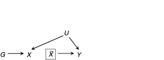
Figure 3: The DAG representing the core conditions under intervention in $\tilde{X}$ and “natural” exposure $X$.

4 Some Common IV Models

With the above core conditions 1–3 and structural assumption of (3.2), the IV can be used to test for the presence of a causal effect, or to derive lower and upper bounds on causal effects for the case when all variables are categorical BalkePearl1994 , Dawid2003 , Manski1990 , Robins1989 . However, for general distributions of $(X,Y,G,U)$, the core conditions alone do not necessarily allow point-identification of causal effects, except for some extremely unusual situations Greenland2000 .

Below we present some common model restrictions, that is, additional parametric assumptions, that enable point-identification of causal parameters. When the causal parameter is identified, it can be estimated consistently; in practice, small sample sizes can still induce problems, but we will ignore this issue here.

Our terminology is as follows. Let $\theta^{*}$ be the true causal parameter of interest, for example, the CRR $\theta^{*}=E_{P^{*}}(Y|\operatorname{do}(x_{2}))/E_{P^{*}}(Y|\operatorname{do}(x_{1}))$, where expectations are taken with respect to the true distribution $P^{*}$. Restrictions are imposed in the form of a statistical model $\mathcal{M}$, which is simply a set of distributions with some common characteristics for the random variables of interest, for example, the conditional mean of $Y$ being linear in $X$. The model $\mathcal{M}$ is correctly specified if $P^{*}\in\mathcal{M}$. The model $\mathcal{M}$ further allows point-identification of the true causal effect parameter when $\theta^{*}$ is equal to a function $\theta_{\mathcal{M}}(P^{*}_{X,Y,G})$ that only depends on the observational (i.e., not interventional) distribution of the observable variables. The exact form of the function $\theta_{\mathcal{M}}$ depends on the model assumptions, that is, on $\mathcal{M}$. If the model $\mathcal{M}$ is misspecified, then it does not contain the true distribution $P^{*}$ and $\theta_{\mathcal{M}}(P^{*}_{X,Y,G})$ will not necessarily be equal to $\theta^{*}$, as the former relies on wrong model assumptions. We call the causal parameters of interest, $\theta^{*}$, the target of inference, and we call $\theta_{\mathcal{M}}(P^{*}_{X,Y,G})$ the estimand regardless of whether the model is correctly specified or not. Hence, the estimand is equal to the target under a correct model and otherwise potentially different. Note that the intervention distribution $P^{*}(Y=y|\operatorname{do}(x))$ itself might be of interest as a target, and, if identified, any causal parameter can be obtained from it.

As we will see below, $\theta_{\mathcal{M}}$ can typically be expressed in terms of conditional probabilities or expectations with respect to the observational distribution of $X,Y$ and $G$. For practical data analysis, these have to be replaced, for instance, by the corresponding empirical relative frequencies, averages or regression coefficients, assuming that we have an independent identically distributed (i.i.d.) sample of $(X,Y,G)$; this then yields an estimator $\hat{\theta}_{\mathcal{M}}$. We will not go into the details of the actual construction of estimators $\hat{\theta}_{\mathcal{M}}$ as functions of the sample but will focus on how different models $\mathcal{M}$ allow point-identification and what the corresponding estimands $\theta_{\mathcal{M}}(P^{*}_{X,Y,G})$ are.

Note that when parametric assumptions are made, the core conditions can sometimes be weakened, for example, by requiring only that $G$ and $U$ are uncorrelated, but we do not discuss this further here. Also, some, but not all, of the following approaches are only defined when $Y$ and/or $G$ are binary. This will be indicated when relevant.

4.1 Linear IV Models

The classical IV method was developed in the context of linear models $\mathcal{M}$ which we define in more detail below, and results in an estimator $\hat{\theta}_{\mathcal{M}}$, given as the ratio of the least squares slope estimators from linear regressions of $Y$ on $G$ and of $X$ on $G$. We will call this the linear IV average effect estimator, and its estimand $\theta_{\mathcal{M}}$ is

$$\mbox{LIVAE}:=\frac{\operatorname{Cov}(Y,G)}{\operatorname{Cov}(X,G)}.$$ (6)

The LIVAE can equivalently be estimated by obtaining predicted values $\hat{X}$ from the regression of $X$ on $G$ and then by regressing $Y$ on $\hat{X}$. It is therefore known as two-stage least squares Angristal1995 , Wooldridge1 . In the special case of binary instrument $G$, we have

$$\mbox{LIVAE}=\frac{E(Y|G=1)-E(Y|G=0)}{E(X|G=1)-E(X|G=0)}.$$ (7)

This is analogous to the Wald method, which was originally proposed to deal with the case of measurement errors in both variables $X$ and $Y$ Boundal1995 , Wald1940 . As we shall now discuss, the LIVAE identifies either the population, individual or local average causal effect (ACE, ICE or LACE), depending on the particular model assumptions.

In addition to the three IV conditions and structural assumption (3.2), assume that the conditional expectation of $Y$ is linear without interactions and that all dependencies only affect the mean. Then

$$\hskip 20.0ptE(Y|X=x,U=u) = E\bigl{(}Y|\operatorname{do}(X=x),U=u\bigr{)}$$

$$= \beta x+h(u),$$

where $h(u)$ is some function of $u$ only. With $\alpha=E(h(U))$, we have

$$E\bigl{(}Y|\operatorname{do}(X=x)\bigr{)}=\alpha+\beta x,$$ (9)

so that the ACE for a unit difference in $X$ is equal to the model parameter $\beta$, while the causal relative risk $\operatorname{CRR}(x_{1},x_{2})$ under this model is equal to $(\alpha+\beta x_{2})/(\alpha+\beta x_{1})$. It can easily be seen (cf. Appendix) that, under the above assumptions, $\beta=\operatorname{Cov}(Y,G)/\break\operatorname{Cov}(X,G)$. Hence, the LIVAE identifies the ACE. In the Appendix we show that the CRR is also identified in this linear model and we will call the corresponding estimand LIVRR.

When $Y$ is binary, for example, assumption (4.1) cannot hold exactly, as it allows $E(Y|X,U)$ to take values outside [$0,1$]. It might still be used as a sensible approximation in practice, especially when the range of $X$ is restricted and its effect is small. As mentioned above, causal relative risks and odds ratios that might be of more interest for binary $Y$ can also be identified based on the linear model as detailed in the Appendix.

Under stronger model assumptions, such as those common in the econometrics literature, for instance, the LIVAE identifies the individual causal effect, ICE. A structural equation model describes how the individual responses $Y^{i}$ depend structurally (i.e., under manipulation) on other variables Pearl2000 , Wooldridge1 . This can also be expressed using counterfactuals Brookhart2007 . A structural equation counterpart for (9) that parameterizes the ICE is given by

$$Y^{i}(x)=\beta_{I}x+\xi^{i}$$ (10)

for individual $i$, where $\xi^{i}$ can be regarded as a combination of $U^{i}$ and other (nonconfounding) factors that determine the outcome. The problem of confounding by $U$ leads to $\xi$ and $X$ not being independent, so that $\beta_{I}$ cannot be estimated consistently from a regression of $Y$ on $X$, and the LIVAE is used instead. For the interpretation it is important to note that model (10) explicitly assumes that the causal effect is the same for each individual $i$, while (4.1) assumes that manipulating $X$ has the same average effect regardless of the value of $U$ on the linear scale. In fact, model (10) implies (4.1), but the converse is not true (see the Appendix for details).

Each of models (4.1) and (10), together with the IV assumptions, allows us to identify the effect of exposure on the exposed, that is, the local average causal effect LACE, via the LIVAE from (6). However, the LACE can be identified under weaker model assumptions, namely, those of an additive structural mean model (cf. the Appendix or Hernan and Robins HernanRobins2006 ). Using the notation introduced in Section 3.1, let $X$ denote the “natural” exposure level, while $\tilde{X}$ denotes the exposure that is set by an intervention (overruling the “natural” $X$). An additive SMM assumes that

$$E(Y|X=x,G=g)$$

$$\quad{}-E\bigl{(}Y|X=x,G=g,\operatorname{do}(\tilde{X}=0)\bigr{)}=\beta_{L}x,$$

where $X=0$ again denotes a suitable baseline value. Here, $\beta_{L}x$ is the effect of reducing the exposure to this baseline value for those who under “natural” circumstances are exposed to $X=x$ and have $G=g$. Note that this additive SMM makes no explicit assumptions about individual causal effects or the role of $U$; in fact, $U$ is allowed to modify the effect of $X$ on $Y$. Implicitly, however, the manner in which $Y$ depends on $U$ is restricted by the assumption that the above difference in conditional expectations (4.1) does not depend on $G$. The different interpretation of the LIVAE in the context of linear models and presence of effect modification is also discussed by Brookhart and Schneeweiss Brookhart2007 .

In summary, we can use the LIVAE to estimate (i) the individual causal effect, if we believe that the individual effect is the same for everyone on the linear scale, or (ii) the average causal effect, if we believe that the average effect is the same for different values of $U$, or (iii) the local effect on the exposed, if we believe that this is the same for different values of $G$.

4.2 Nonlinear Wald Type Methods

As mentioned earlier, the LIVAE is the same as Wald’s estimator which was originally devised to deal with measurement errors Wald1940 . In this section we consider two further methods leading to ratio based IV estimators and which we will therefore call Wald type estimators (cf. also Lawloral2008a , Minellial2004 , Thompsonal2005 ).

Several applications of Mendelian randomization, typically considering a binary outcome $Y$, a continuous exposure $X$ and a dichotomous genotype $G$, have used the following reasoning to obtain an IV estimator for a causal effect Casasal2005 , Casasal2006 , DaveySmithEbrahim2003 , Keavneyal2006 , Lawloral2008b . The naïve odds ratio of $Y$ given $X$, which we denote NOR, is suspected to be confounded. The odds ratio of $Y$ given the instrument $G$, which we denote by $\operatorname{OR}(Y|G)$, is not confounded due to core condition 3, and should be roughly equal to the causal odds ratio, COR, between $X$ and $Y$ scaled by the mean difference in exposure for the two genotypes, $\delta=E(X|G=1)-E(X|G=0)$, that is, $\operatorname{OR}(Y|G)\approx$ COR^δ. Therefore, in these applications, the quantity NOR^δ is compared with $\operatorname{OR}(Y|G)$ and, if similar, the conclusion is drawn that there is no confounding and, hence, that NOR $\approx$ COR. We thus consider the following as the Wald type odds ratio estimand:

$$\mbox{WaldOR}:=\operatorname{OR}(Y|G)^{1/\delta}.$$

(On the log-scale this is the ratio of log-odds difference and the mean difference $\delta$, hence “Wald type.”) At first sight, this reasoning seems heuristic, and there is no model assumption from which it can be theoretically derived. However, by regarding the odds ratio as an approximation to the relative risk for rare diseases, we can motivate the above formula theoretically. The following is a slight generalization of the structural equation approach presented by Mullahy Mullahy1997 and suitable not only for binary but also for general nonnegative response $Y$ ($X$ and $G$ can be continuous or discrete). Assuming a log-linear model [and structural assumption (3.2)],

$$\log E(Y|X=x,U=u)$$

$$\quad=\log E\bigl{(}Y|\operatorname{do}(X=x),U=u\bigr{)}$$ (12)

$$\quad=\gamma x+h(u),$$

where $h(u)$ is some function of $u$ only. It can then easily be seen that the causal relative risk for one unit difference in $X$ is simply $\operatorname{CRR}=\exp\gamma$. Further, we suppose that $X$ has conditional mean

$$E(X|G=g,U=u)=\delta g+k(u),$$ (13)

where $k(u)$ is some function of $u$ only, and, in addition, we require that the distribution of $X$ is such that

$$\bigl{[}X-\bigl{(}\delta G+k(U)\bigr{)}\bigr{]}\perp\!\!\!\!\perp G|U.$$ (14)

Note that this requirement cannot be satisfied when $X$ is binary, for instance, but is automatically true when it has a conditional normal distribution. It can now be shown (cf. the Appendix or Mullahy Mullahy1997 ) that the CRR is identified because $\gamma$ is equal to the ratio of the log-coefficient from a loglinear regression of $Y$ on $G$ and the coefficient from a linear regression of $X$ on $G$. In the special case of a binary instrument $G$, this simplifies to

$$\gamma=\frac{\log E(Y|G=1)-\log E(Y|G=0)}{E(X|G=1)-E(X|G=0)}.$$

The method of estimating this via two regressions as mentioned above is also called two-stage quasi maximum likelihood Mullahy1997 . We will refer to the estimand based on the right-hand side of the above as the Wald relative risk (WaldRR), given by

$$\operatorname{WaldRR}:=\operatorname{RR}(Y|G)^{1/\delta},$$

where $\operatorname{RR}(Y|G)$ is shorthand for the relative risk of $Y$ given $G$. When $G$ is binary, $\delta$ is the mean difference in $X$, otherwise it is $\operatorname{Cov}(X,G)/\operatorname{Var}(G)$.

The WaldRR identifies the CRR under the above combination of log-linear model for $Y$ given $X$ and $U$, and the stated assumptions on the conditional distribution of $X$ given $G$ and $U$. Note that when $Y$ is nonnegative and continuous, it is, in principle, possible (but not common) to elaborate the assumptions further so that the individual relative causal effect $Y^{i}(x_{2})/Y^{i}(x_{1})$ is identifiable; model (4.2) would then need to be reformulated as a structural equation model analogously to the linear case earlier.

When $Y$ is binary and $P(Y=1)$ is small (“rare disease assumption”), WaldRR and WaldOR will be approximately the same, so that in this case we can argue that the WaldOR approximately identifies the COR under the same model assumptions. A different justification of WaldOR has been proposed by Babanezhadal2009 based on a logistic SMM and some very rough approximations, under which it identifies the LCOR.

4.3 Multiplicative Structural Mean Models

We already mentioned that the LIVAE can be justified in an additive SMM identifying the causal mean difference within the exposed individuals (LACE). Alternatively, we now consider a multiplicative structural mean model (MSMM) HernanRobins2006 . Again using the notation introduced in Section 3.1, let $X$ denote the “natural” exposure level, while $\tilde{X}$ denotes the exposure that is set by an intervention (overruling the “natural” $X$). An MSMM parameterizes the LCRR (2) and is given by

$$\log\biggl{\{}\frac{E(Y|X=x,G,\operatorname{do}(\tilde{X}=x))}{E(Y|X=x,G,\operatorname{do}({\tilde{X}}=0))}\biggr{\}}=\gamma_{L}x,$$ (15)

where ${\tilde{X}}=0$ stands for a suitable baseline value as before. Hence, $\gamma_{L}x$ is the log-relative risk of changing the exposure to this baseline for those who would normally be exposed to $X=x$, where it is assumed that the effect is the same within different levels of the instrument $G$. This does not follow from the core IV conditions nor from the structural assumption (3.2). It means, for example, that reducing the alcohol intake for those individuals who are heavy drinkers has the same effect on the relative risk for hypertension regardless of their ALDH2 genotype. This may be unrealistic if those who drink much despite carrying the ALDH2*2 variant are different in relevant aspects from those who drink much and do not carry this allele. An analogous assumption is made by the additive SMM (4.1) but for the risk difference; note that except for trivial cases both, the assumption that $G$ does not modify the effect on the multiplicative and on the additive scale, cannot be true at the same time HernanRobins2006 . This assumption of no heterogeneity with respect to levels of $G$ is required so that the model has only one unknown parameter, since we can only identify one parameter. When baseline covariates have been measured, it is possible to identify more complex SMMs and this assumption could be relaxed Babanezhadal2009 , Fischeral2004 , HernanRobins2006 , but we do not consider this any further here.

In general, a SMM estimator for a causal parameter is obtained by solving estimating equations that are based on the exclusion restriction mentioned in Section 3.2. The solution typically does not have a closed form expression. However, for the case where $X$ and $G$ are binary, an explicit solution exists HernanRobins2006 , Robins1989 (cf. also the Appendix), yielding that $\exp(-\gamma_{L})$ equals

$$1-\frac{E(Y|G=1)-E(Y|G=0)}{E(YX|G=1)-E(YX|G=0)}.$$ (16)

The parameter $\gamma_{L}$ can easily be estimated using the corresponding empirical frequencies or averages. Under the multiplicative SMM, we hence obtain that the estimand is the inverse of (16), which we will call MSMMRR. It identifies the LCRR under the IV core conditions and the assumptions of an MSMM. In order for it to also identify the population effect CRR, it is sufficient to assume that $X$ and $U$ cannot interact on $Y$ on the multiplicative scale HernanRobins2006 . This is analogous to the “no interaction” assumption in linear model (4.1). In this special case we can also obtain closed formulae for the odds ratio and risk difference HernanRobins2006 , Robins1989 (cf. also the Appendix).

Table 1: Summary of IV model assumptions under which the various estimands identify the targeted causal effects(in addition to general IV assumptions)

Estimand	Target	Model assumptions
LIVAE	ICE	Constant additive individual effect [$Y^{i}(x)$ linear in $x$].
LIVAE	ACE	$E(Y|X=x,U=u)$ linear in $x$, no $(X,U)$-interaction on additive scale.
LIVAE	LACE	$E(Y|X=x,G=g)-E(Y|X=x,G=g,\operatorname{do}(\tilde{X}=0))$ linear in $x$, no $(X,G)$-interaction on additive scale.
LIVRR	CRR	Same as LIVAE for ACE.
WaldRR	CRR	(i) $E(X|G=g,U=u)$ linear in $g$, no $(G,U)$-interaction on additive scale, additive independent residual. (ii) $E(Y|X=x,U=u)$ log-linear in $x$, no $(X,U)$-interaction on multiplicative scale.
MSMMRR	LCRR	$\log\{E(Y|X=x,G=g)/E(Y|X=x,G=g,\operatorname{do}(\tilde{X}=0))\}$ linear in $x$, no $(X,G)$-interaction on multiplicative scale.
MSMMRR	CRR	As for LCRR, and no $(X,U)$-interaction on multiplicative scale.

Logistic structural mean models have been proposed VansteelandtGoetghebeur2003 , but these require more restrictive assumptions, and conditions enabling consistent estimation are relatively complicated. We therefore omit them here. Robins and Rotnitzky RobinsRotnitzky2004 provide a detailed discussion of the fundamental difficulty with identifiability in SMMs, other than for the additive or multiplicative cases.

4.4 Comparison of Assumptions

The estimands, their target causal effects and the conditions for identification are summarized in Table 1. (WaldOR as an approximation to WaldRR is omitted.) The following points are noteworthy:

• One could say that the strongest assumptions are those underlying the WaldRR and WaldOR, as they rely on a specific outcome model for the distribution of $Y$ given $(X,U),$ as well as a specific exposure model for the distribution of $X$ given $(G,U)$. Neither the linear models nor the SMMs require the latter.

• All IV approaches underlying point-estimation rely on some “no-interaction” (or homogeneity/no effect modification assumption). No interaction between $X$ and $U$ on the linear (or log-linear) scale in the sense of model (4.1) [or model (4.2)] is sufficient to ensure the assumption of no interaction between $X$ and $G$ in the additive (or multiplicative) SMMs, models (4.1) and (15) (see the Appendix). However, the “no-interaction” assumption may either be true on the linear or on the log-linear scale, but not both, except in trivial cases like $Y\perp\!\!\!\!\perp X|U$ or $Y\perp\!\!\!\!\perp U|X$ HernanRobins2006 .

• In contrast to the MSMM, the linear and Wald-type models do not require joint information on $(X,Y,G)$; they allow identification of the causal parameter based on separate information on the joint distribution of $(X,G)$ and of $(Y,G)$, only. This means that an IV analysis can be performed by exploiting results, for example, from different existing genetic studies or meta-analyses as is particularly relevant for Mendelian randomization applications Minellial2004 , Thompsonal2005 . In addition, the WaldOR is useful for case-control studies where, under the rare disease assumption, $\delta$ can be approximated by a control group estimate Keavneyal2006 .

5 Numerical Illustration ofAsymptotic Bias

In the previous section we have given some examples of standard models that allow point-identification of a causal parameter exploiting an IV. In practice, such model assumptions are unlikely ever to hold exactly, and we should be concerned with the robustness of IV methods under violations of such assumptions. Therefore, in this section we illustrate the possible bias of the above approaches for a set of concrete scenarios that would be realistic, for instance, in a Mendelian randomization study. We place importance on the following issues:

• A sensible IV model should allow consistent estimation at the null-hypothesis of no causal effect.

• A sensible IV model should also allow consistent, or at least not seriously biased, estimation when there is in fact no confounding, and hence a “naïve” analysis, based on a regression of response $Y$ on exposure $X$ without using an IV, would be valid.

• A sensible IV model should also not induce more bias than such a naïve approach.

We want to investigate which of the various IV methods satisfy these desiderata, or what situations lead to the most serious violations.

Using the notation introduced at the beginning of Section 4, we base our comparison on the difference between the targeted causal parameter $\theta^{*}$ and the estimand $\theta_{\mathcal{M}}$ under a given model $\mathcal{M}$, evaluated at the true distribution $P^{*}$. More precisely, we use the relative measure

$$\frac{\theta_{\mathcal{M}}-\theta}{\theta},$$

which is the asymptotic relative bias of any consistent estimator $\hat{\theta}_{\mathcal{M}}$ for $\theta_{\mathcal{M}}$. If the model is correctly specified, that is, $P^{*}\in\mathcal{M}$, and identifies the causal parameter, then the above is zero. The asymptotic relative bias can be calculated exactly, using numerical integration where required, under a given choice of a “true” joint distribution $P^{*}$ of $(X,Y,G,U)$ (see below). In special cases it is even possible to express the bias explicitly as in Brookhart2007 for the linear case. Note that we are not considering any sampling properties of specific estimators $\hat{\theta}_{\mathcal{M}}$ and hence are not simulating any data.

We restrict our numerical comparison to the causal relative risk, $\theta^{*}=\operatorname{CRR}$, as target. We compare the linear model, with estimand LIVRR, the log-linear Wald type approach, with estimand WaldRR (WaldOR is always slightly more biased for CRR than WaldRR and is therefore omitted), and the multiplicative SMM, with estimand MSMMRR, which all identify the CRR under their respective assumptions as detailed in Section 4.

5.1 Full Model

The true joint distributions $P^{*}$ for $(X,Y,G,U)$ that we use for the comparison are specified as follows. To facilitate interpretation and to keep the number of parametric and distributional choices limited, we consider dichotomous observable variables $Y$, $X$ and $G$ with the following interpretations:

$$Y = \cases{1,&diseased,\cr 0,&healthy,}$$

$$X = \cases{1,&exposed,\cr 0,&not exposed,}$$

and we label $G=1$ to denote the value of the instrument that predisposes to $X=1$.

The dependence of $Y$ on $X$ and $U$ is given by a logistic regression. In addition, we assume that this model is invariant with respect to intervention on $X$, by which we mean

$$\operatorname{logit}E(Y|X=x,U=u)$$

$$\quad=\operatorname{logit}E\bigl{(}Y|\operatorname{do}(X=x),U=u\bigr{)}$$ (17)

$$\quad=\alpha_{1}+\alpha_{2}x+\alpha_{3}u+\alpha_{4}xu.$$

The conditional distribution of $X$ given $G$ and $U$ is also determined by a logistic dependence:

$$\operatorname{logit}E(X|G=g,U=u)$$

(18)

$$\quad=\beta_{1}+\beta_{2}g+\beta_{3}u+\beta_{4}gu.$$

Finally, the marginal distribution of $G$ is determined by $p_{g}=P(G=1)$, which we set to 50% throughout (all estimands are unaffected by $p_{g}$), while $p(u)$ is continuous and set to have a uniform distribution on $[0,1]$.

The true CRR can easily be calculated from the above using (3.2) and integrating out as

$$\frac{\int\{1+\exp(-\alpha_{1}-\alpha_{2}-\alpha_{3}u-\alpha_{4}u)\}^{-1}p(u)\,du}{\int\{1+\exp(-\alpha_{1}-\alpha_{3}u)\}^{-1}p(u)\,du}.$$ (19)

Note that the CRR does not depend on (5.1), but $\theta_{\mathcal{M}}$ does for the IV models considered here.

For the above true distributions $P^{*}$, all models from Section 4 are essentially misspecified, since none of them model a logistic dependence of $Y$ on $(X,U)$. Exceptions are $\alpha_{2}=\alpha_{4}=0$, or for the linear and MSMM when $\alpha_{3}=\alpha_{4}=0$. Also, note that if $\alpha_{4}=0$, then there is no effect modification by $U$ on the logistic scale. This does not strictly imply no effect modification on the additive or multiplicative scales, though departure from these assumptions will be more extreme when $\alpha_{4}\not=0$.

Our choice of $P^{*}$ is motivated by the fact that a logistic model like (5.1) would be the standard model assumption for a binary outcome if the confounder(s) $U$ could be observed. It is noteworthy that this default model assumption for the case of observed confounding is not necessarily compatible with standard IV methods for unobserved confounding.

5.1.1 Settings of the parameters

There are eight parameters in (5.1) and (5.1). By varying these, we consider the following set of scenarios which we regard as realistic for epidemiological studies based on Mendelian randomization, for example.

We choose three strengths for the causal effect: none $(\operatorname{CRR}=1.0)$, small $(\operatorname{CRR}=1.33)$ and large $(\operatorname{CRR}=3.03)$; this is obtained by adjusting $\alpha_{2}$ accordingly. Confounding is varied by setting $\alpha_{3}\in\{0,\break 0.1,1,2\}$, while keeping $\beta_{3}=2$ fixed. Interactions are investigated by varying $\beta_{4},\alpha_{4}\in\{-1,0,1\}$, but note that we only consider combinations where $|\alpha_{4}|\leq|\alpha_{3}|$, as large interactions with small main effects are commonly perceived as unrealistic. The remaining parameters are chosen so as to satisfy the following criteria. The strength of the association between $G$ and $X$ is kept constant at a relative risk of 2.4 throughout by adjusting $\beta_{2}$ accordingly. We fix the marginals $P(X=1)=0.13$ and $P(Y=1)=0.03$ by setting $\beta_{1}$ and $\alpha_{1}$ accordingly. These latter values, respectively, are again typical for the exposure frequencies and rare disease situations, as are often encountered in Mendelian randomization studies.

5.1.2 Bounds

To further characterize the chosen scenarios, we calculated the nonparametric bounds for the CRR (and the ACE for comparison) BalkePearl1994 , Dawid2003 , Manski1990 , Robins1989 for all our settings and found that they were always extremely wide and always included the null hypothesis of no effect. For those settings where $\operatorname{CRR}=3.03$, for instance, the bounds were of the order [$0.2,30$] (and about [$-0.08,0.8$] for the ACE where the true ACE was around 0.06). These are the “tightest assumption-free bounds” BalkePearl1994 , meaning that the observable frequencies $p(y,x,g)$ alone, derived from the above distributions by marginalizing over $U$, do not allow us to narrow down the causal effects any further. This re-emphasizes the fact that point-identification via an IV model relies heavily on the additional parametric assumptions that have to be made. Narrower bounds can be obtained when a stronger instrument is used, that is, by increasing the $G$–$X$ association. However, the relative risk of 2.4 used here is about as strong as we would expect to see in a Mendelian randomization study.

5.2 Numerical Results

We now compare the asymptotic biases of the LIVRR, WaldRR and MSMMRR. In addition, we consider the naïve relative risk, NRR, obtained as $P^{*}(Y=1|X=1)/P^{*}(Y=1|X=0)$, which gives an indication of the bias of a standard analysis when not using an IV. In our settings, the NRR is unbiased when there is no confounding, but not necessarily otherwise.

5.2.1 No causal effect

We begin with the case where $\operatorname{CRR}=1$, which usually constitutes the null hypothesis. When $\alpha_{4}=\alpha_{2}=0$, no table is shown as none of the IV models from Section 4 are misspecified, only the NRR is biased by as much as 39%. However, $\operatorname{CRR}=1$ can also arise when $\alpha_{2}$ and $\alpha_{4}$ are nonzero and of opposite signs. The relative biases for the corresponding settings are shown in Table 2.

Table 2: Asymptotic relative biases when estimating CRR for all settings with $\operatorname{CRR}=1$ and $\alpha_{4}\not=0$

			Relative bias
$\bolds{\alpha_{3}}$	$\bolds{\alpha_{4}}$	$\bolds{\beta_{4}}$	NRR	LIVRR	WaldRR	MSMM
1	$1$	$0$	$0.277$	$0.105$	$0.110$	$0.095$
2			$0.414$	$0.092$	$0.095$	$0.075$
1	$-1$		$0.020$	$-0.113$	$-0.108$	$-0.101$
2			$0.174$	$-0.106$	$-0.102$	$-0.087$
1	$1$	$1$	$0.361$	$0.198$	$0.213$	$0.163$
2			$0.545$	$0.177$	$0.189$	$0.125$
1	$-1$		$0.025$	$-0.202$	$-0.187$	$-0.169$
2			$0.226$	$-0.195$	$-0.181$	$-0.140$
1	$1$	$-1$	$0.184$	$0.006$	$0.006$	$0.006$
2			$0.272$	$0.002$	$0.002$	$0.002$
1	$-1$		$0.013$	$-0.009$	$-0.009$	$-0.009$
2			$0.115$	$-0.006$	$-0.006$	$-0.005$

The problem we mentioned earlier, and that becomes evident here, is that there can be two types of scenarios where $\operatorname{CRR}=1$: either there is no causal effect of exposure in any subgroup ($\alpha_{2}=\alpha_{4}=0$), or there are different causal effects in subgroups which cancel out overall. The latter occurs when $\alpha_{2}$ and $\alpha_{4}$ are nonzero in such a way that the ratio of integrals in (19) happens to be one.

All IV methods exhibit some bias in these scenarios, with around 20% relative bias in the worst case. We can see the following patterns in Table 2. When $\beta_{4}=-1$, all IV estimators are only slightly biased, while the NRR can be biased by up to 27%. There are only two settings where all IV methods are more biased than the naïve one, and these are when $\alpha_{4}=-1$ and $\alpha_{3}=1$, and $\beta_{4}=0$ or 1. For all considered settings, the MSMMRR is the least biased, and the WaldRR is the most biased, but the order of magnitude is generally comparable and we would not suggest an overall ranking of the approaches based on these results alone.

Recall that the MSMMRR does not actually target the CRR, but targets a particular subgroup effect—the local causal relative risk of exposure within the exposed—instead. The latter is typically not one when $\alpha_{2}\not=0$.

5.2.2 Causal effect but no confounding

Let us now consider those scenarios where there is no confounding (so either $\alpha_{3}=\alpha_{4}=0$ or $\beta_{3}=\beta_{4}=0$). No plots or tables are shown here as only the WaldRR has nonzero bias. This is because all assumptions of the naïve, linear and multiplicative structural mean models are satisfied when there is no confounding and when $X$ and $Y$ are binary. In contrast, as noted in Section 4.2 and again in the Appendix, the assumption (14) underlying the WaldRR cannot be satisfied when $X$ is binary. We observed biases for the WaldRR and WaldOR of up to $3.2$% and $4.5$%, respectively, for a moderate effect size of $\operatorname{CRR}=1.33$, and biases as large as $65$% and $76$%, respectively, when $\operatorname{CRR}=3.03$.

5.2.3 Causal effect and confounding

We now consider those scenarios where there is a causal effect as well as confounding. Tables 3 and 4 show the results for a small causal effect ($\operatorname{CRR}=1.33$) and a large causal effect ($\operatorname{CRR}=3.03$), respectively.

Table 3: Asymptotic relative biases when estimating CRR for all settings with $\operatorname{CRR}=1.33$

			Relative bias
$\bolds{\alpha_{3}}$	$\bolds{\alpha_{4}}$	$\bolds{\beta_{4}}$	NRR	LIVRR	WaldRR	MSMM
0.1	$0$	$0$	$0.015$	$0.003$	$0.036$	$-0.000$
1.0			$0.150$	$0.027$	$0.066$	$-0.001$
2.0			$0.299$	$0.051$	$0.097$	$-0.002$
1.0	$1$	$0$	$0.275$	$0.130$	$0.206$	$0.093$
2.0			$0.411$	$0.141$	$0.222$	$0.072$
1.0	$-1$	$0$	$0.020$	$-0.085$	$-0.071$	$-0.101$
2.0			$0.172$	$-0.052$	$-0.033$	$-0.088$
0.1	$0$	$1$	$0.019$	$0.005$	$0.038$	$-0.000$
1.0			$0.195$	$0.048$	$0.095$	$-0.002$
2.0			$0.392$	$0.096$	$0.160$	$-0.004$
1.0	$1$	$1$	$0.358$	$0.247$	$0.380$	$0.159$
2.0			$0.541$	$0.273$	$0.422$	$0.120$
1.0	$-1$	$1$	$0.025$	$-0.153$	$-0.148$	$-0.169$
2.0			$0.225$	$-0.100$	$-0.089$	$-0.142$
0.1	$0$	$-1$	$0.010$	$0.000$	$0.032$	$0.000$
1.0			$0.100$	$0.001$	$0.034$	$0.000$
2.0			$0.197$	$0.002$	$0.034$	$0.000$
1.0	$1$	$-1$	$0.182$	$0.004$	$0.039$	$0.005$
2.0			$0.270$	$0.002$	$0.032$	$0.002$
1.0	$-1$	$-1$	$0.013$	$-0.004$	$0.027$	$-0.009$
2.0			$0.114$	$-0.000$	$0.034$	$-0.006$

First, let us compare the results for small versus large CRR. The naïve relative risk (NRR) behaves similarly in both cases. The LIVRR is more biased when the true causal effect is large—this is plausible as the nonlinearity of the model is more pronounced for larger causal effects. The WaldRR is unacceptable when $\operatorname{CRR}=3.03$: with relative biases between 40% and 250%, it seriously overestimates the true effect. As its bias is either comparable to, or much larger than, the bias for the other two IV methods when $\operatorname{CRR}=1.33$, we will not consider the WaldRR any further. The relative bias of the MSMMRR, in turn, is similar for small and large CRR with a maximum of 17%.

As one might expect, the LIVRR and MSMMRR are only slightly biased, and much less so than the NRR, whenever there is no $X$–$U$ interaction, $\alpha_{4}=0$. More surprising is that this is also the case when $\beta_{4}=-1$ regardless of the other parameter values. This is not due to less confounding, as we can see that the naïve relative risk is still noticeably biased in those settings.

All methods struggle the most when $\alpha_{4}\not=0$ and $\beta_{4}=1$—the MSMMRR bias then reaches 17% and the extent of the LIVRR bias can range from 24% for small CRR to 45% for large CRR.

Even though there is no uniformly best method, both tables show that the MSMMRR is much less biased in most settings. The only cases where it is outperformed by the LIVRR arise when $\alpha_{4}=-1$. The only cases where it is outperformed by the NRR are when additionally $\alpha_{3}=1$.

Table 4: Asymptotic relative biases when estimating CRR for all settings with $\operatorname{CRR}=3.03$

			Relative bias
$\bolds{\alpha_{3}}$	$\bolds{\alpha_{4}}$	$\bolds{\beta_{4}}$	NRR	LIVRR	WaldRR	MSMM
0.1	$0$	$0$	$0.014$	$0.006$	$0.671$	$-0.001$
1.0			$0.145$	$0.066$	$0.870$	$-0.006$
2.0			$0.289$	$0.128$	$1.090$	$-0.010$
1.0	$1$	$0$	$0.265$	$0.161$	$1.220$	$0.084$
2.0			$0.397$	$0.210$	$1.410$	$0.061$
1.0	$-1$	$0$	$0.020$	$-0.036$	$0.539$	$-0.102$
2.0			$0.167$	$0.033$	$0.757$	$-0.093$
0.1	$0$	$1$	$0.018$	$0.013$	$0.695$	$-0.001$
1.0			$0.188$	$0.132$	$1.110$	$-0.010$
2.0			$0.379$	$0.263$	$1.630$	$-0.017$
1.0	$1$	$1$	$0.344$	$0.334$	$1.950$	$0.144$
2.0			$0.523$	$0.447$	$2.510$	$0.102$
1.0	$-1$	$1$	$0.025$	$-0.070$	$0.440$	$-0.170$
2.0			$0.217$	$0.062$	$0.858$	$-0.150$
0.1	$0$	$-1$	$0.009$	$-0.001$	$0.647$	$-0.000$
1.0			$0.096$	$-0.006$	$0.637$	$-0.000$
2.0			$0.191$	$-0.014$	$0.605$	$-0.000$
1.0	$1$	$-1$	$0.176$	$-0.019$	$0.590$	$0.005$
2.0			$0.261$	$-0.028$	$0.570$	$0.003$
1.0	$-1$	$-1$	$0.013$	$0.004$	$0.663$	$-0.009$
2.0			$0.110$	$-0.002$	$0.648$	$-0.006$

5.2.4 Sign of bias

Due to our choices of the coefficients of $U$, the NRR is always positively biased. The IV estimators can, however, be negatively biased, especially when $\alpha_{4}$ or $\beta_{4}$ are negative. Also, their bias does not always have the same sign. Therefore, we cannot say that IV methods generally over- or underestimate the true causal effect.

5.2.5 Other comparisons

We also considered the other causal parameters, ACE and COR, as targets in our chosen scenarios using the corresponding estimands under the three IV models. We got broadly similar results with the SMM approach generally producing less biased results, except in the presence of interactions, and the Wald approach behaving very poorly throughout even when there is little or no confounding.

All results presented so far were for scenarios with 3% disease frequency and 13% exposure frequency. We also considered scenarios with 20% disease and/or 50% or 85% exposure frequencies, but do not report them in detail as the results followed similar patterns in terms of relative performances of the various approaches. All IV methods show much less bias with 50% exposure frequency, with the WaldRR performing much more sensibly, in particular. The MSMM is still clearly the least biased and is not sensitive to interaction effects when the exposure frequency is 50%. This might be due to the exposure distribution being more balanced, so that conditioning on $X$ is not so informative for $U$ and, hence, the local causal effect is not much different from the population causal effect even when there are strong interactions.

5.3 Practical Implications

In Section 4.4 we compared the assumptions underlying the IV models of Section 4 on theoretical grounds. The above numerical study adds the following insights:

• The linear IV approach is often not considered appropriate when the outcome variable is binary or nonnegative. However, we found that it performed better than expected for binary $Y$ with relative asymptotic bias below 20% in all but six of the considered scenarios and with less bias than that of the naïve approach in all but five scenarios. This may be deemed acceptable, especially given the simplicity of the linear IV estimator. However, for the linearity assumption to be at least approximately appropriate with binary outcomes, the range of exposure $X$ should be restricted and the true causal effect small. The latter is not uncommon for epidemiological—especially Mendelianrandomization—applications.

• Although it is clear by theory alone that the Wald type methods from Section 4.2 make very strong assumptions, we have seen here that they are not just slightly but can be extremely biased when these assumptions are violated. It is especially worrisome that this occurs for realistic scenarios, that the bias can be worse than with the naïve approach and increases with the strength of the true causal effect, and that they can be biased even when there is no confounding since the model for the exposure $X$ is violated. We would therefore not recommend this approach unless there is good reason to be confident in the model assumptions. A small true causal effect and a balanced or approximately normal distribution of the exposure $X$, possibly after suitable transformation, would support this confidence.

• As mentioned before, all IV approaches, excluding the bounds, make an assumption of no-interaction or no effect modification by the unobserved confounder $U$ either on the additive or multiplicative scale. The results show that violation of this assumption indeed seriously increases the bias of all IV methods and can lead to bias even at the null hypothesis of no causal effect. In practice, this assumption is difficult to asses or justify, as it involves the unobserved confounders which might include factors that are poorly understood.

• As far as the relative bias is concerned, the MSMM approach seems the most recommendable for situations similar to those of Section 5.1, especially for binary outcomes. However, other properties are relevant for practical application, most important being the efficiency of the estimators. As our numerical study only considers a specific set of scenarios, it is also not possible to say whether the MSMM performs equally well in very different situations. We therefore recommend that further comparison and sensitivity analyses are carried out for any specific application.

6 Conclusion and Discussion

Our theoretical comparison of different IV methods was motivated by the need for such methods in observational epidemiology, with Mendelian randomization applications providing an example that has generated a lot of recent interest. The core conditions 1–3 plus the structural assumption (3.2) are sufficient for testing for a causal effect of exposure on disease, but, as emphasized here, the identification of a causal effect has to rely on additional model assumptions which, if inappropriate, can induce bias as illustrated in our numerical study. The need for a comparison of IV methods is also highlighted by the results of a recent study which concluded that there were very few differences between IV approaches because they yielded similar results on particular data sets Rassenal2009b , Rassenal2009a . Our results do not support this point of view and show that any model assumptions have to be justified carefully.

The main points to be made from our comparison are that the different IV approaches target different parameters, where we are not referring to the difference between a risk difference and risk ratio, for instance, but the difference between an individual, population or local causal effect. In the case of the latter, the SMM approach (additive or multiplicative) makes the weakest assumptions, as it does not require a model for the exposure $X$ given the instrument $G$, and it only assumes (log-)linearity of the effect within the exposed individuals. Under stronger assumptions, essentially if $U$ and $X$ do not interact on $Y$ on the relevant scale, the local causal effect is equal to the population causal effect. However, the multiplicative SMM requires joint data on the observable variables which may not always be available from existing studies. For the linear model it has also been noted by Brookhart2007 that the traditional ratio estimator LIVAE has to be given a different interpretation in the presence of effect modification. The Wald type estimator for the relative risk, together with the odds ratio as an approximation to the latter, is simple and useful for meta-analyses but makes very specific assumptions about all conditional distributions, especially that of the exposure, and also requires the absence of interactions on the multiplicative scale.

Our bias calculations are of course only valid for the particular model and scenarios we chose to consider, but we believe they still raise serious issues. Not surprisingly, all estimators encounter difficulties in estimating the population effect in scenarios where the exposure has different effects within levels of the unobserved confounder. Maybe more surprising are the particularly poor performances of the Wald relative risk and odds ratio—especially in the absence of confounding. This is supported by a recent study on odds ratio estimators which also found that the WaldOR was often outperformed by other approaches Babanezhadal2009 . However, we did not find that it did “especially well” at the causal null hypothesis, as reported there, when there were interactions in the model for the outcome $Y$. An obvious implication for practical applications of IV methods is that the plausibility of such interactions, on the chosen effect scale, should be explicitly addressed. If such interactions are judged to be likely on the multiplicative scale, then the MSMM estimator is closer to the local effect and the Wald relative risk is likely to be seriously biased. Also, one has to keep in mind that such interactions can induce bias of all IV methods even at the null hypothesis of no causal effect, though one might hope that such exact cancellations of subgroup effects are rare. It might be argued that, in practice, important effect modifiers will be known and observed as additional covariates, so that once these are taken into account, only negligible interactions with the unobserved confounders remain, but by definition this cannot be verified empirically. Note that any justification for the absence of effect modification has to take the chosen measurement scale into account. Due to the increased bias we have seen in our numerical study, we would therefore recommend that practical applications of IV methods be complemented by some sensitivity analyses, especially with regard to such interactions in the model for the outcome $Y$. Moreover, we would advise that these considerations are also valid for continuous outcomes which are often analyzed unquestioned with linear no-interaction models.

The particularly restrictive assumptions underlying the WaldRR (and WaldOR) raise serious concern about how to handle situations where we do not have joint information on all the relevant variables, such as in most meta-analyses, rendering the multiplicative SMM estimator inapplicable. The linear IV estimator could, in principle, be applied, as it too does not require joint data and is not as badly biased, but for binary disease outcomes, risk differences are rarely reported. In most applications the exposure is continuous and robustness of the nonlinear Wald estimators to violations in those cases remains to be investigated. It certainly does not seem advisable to dichotomize a continuous exposure.

We have only considered the asymptotic bias of the various estimators. In practice, their efficiency will also be of major concern. It is well known that IV estimators have larger variance than the naïve estimators when there is no unobserved confounding. The variance, unlike the bias, very much depends on the strength of the instrument, but when there is strong confounding, it is impossible to find a strong instrument Boundal1995 , Martensal2006 . The SMM estimators, derived from estimating equations, can be made semi-parametrically efficient by choosing appropriateweights in these equations Robins1994 . Some methods for improving the efficiency of the Wald type relative risk have been proposed Mullahy1997 . Further comparisons of properties and sampling behavior of IV estimators for the special case of a binary outcome can be found in Babanezhadal2009 , ClarkeWindmeijer2009 .

Another important issue that we have not addressed here is that of measurement error. Theoretically, it is not a problem if the IV is affected by measurement error, as long as this is not differential. If the exposure is affected by measurement error, we can still use the IV approach to test for a causal effect. However, all the above IV estimators are then expected to be biased, as core condition 3 is likely to be violated when $X$ is the measured, and not the true, exposure. In that case, we have to make even more modeling assumptions, namely, about the specific measurement error process, in order to obtain valid point estimates VansteelandtBabanezhadGoetghebeur2007 .

Appendix

Justification of LIVAE

We have established that the ACE is equal to the model parameter $\beta$ in model (4.1). Define $\tilde{G}=G-E(G),$ then $E(Y\tilde{G})=\operatorname{Cov}(Y,G)$. With core condition 1 and model (4.1),

$$E(Y\tilde{G}) = E_{G}E(Y\tilde{G}|G)$$

$$= E_{G}\bigl{(}\beta E(X\tilde{G}|G)+\tilde{G}E(h(U))\bigr{)}$$

$$= \beta E(X\tilde{G}).$$

Hence, $\beta=\operatorname{Cov}(Y,G)/\operatorname{Cov}(X,G)$, which is theLIVAE estimand.

Risk ratios or odds ratios require estimation of the intercept of (9) obtained as follows:

$$\hat{\alpha}=E(Y)-\hat{\beta}E(X),$$

where $\hat{\beta}=\mbox{ LIVAE}$ from above. Hence, the CRR and COR are identified by

LIVRR $$:= \frac{\hat{\alpha}+\hat{\beta}}{\hat{\alpha}},$$

LIVOR $$:= \frac{(\hat{\alpha}+\hat{\beta})(1-\hat{\alpha})}{\hat{\alpha}(1-\hat{\alpha}-\hat{\beta})}.$$

Further, under the additive SMM (4.1) we have by simple rearranging that $E(Y|X,G,\operatorname{do}(\tilde{X}=0))=E(Y-\beta_{L}X|X,G)$, where we use that $E(Y|X=\break x,G,\operatorname{do}(\tilde{X}=x))=E(Y|X=x,G)$. The exclusion restriction implies that $Y\perp\!\!\!\!\perp G|\operatorname{do}(\tilde{X}=0)$ (cf. Figure 2), which induces an estimating equation to obtain $\beta_{L}$ based on the moment condition $E((Y-\beta_{L}X)\tilde{G})=0$, where $\tilde{G}=G-E(G)$, as before. The solution is again $\beta_{L}=\operatorname{Cov}(Y,G)/\operatorname{Cov}(X,G)$.

Justification of WaldRR

In addition to the model assumptions expressed in (4.2) and (13), we need (14), that is, the random variable $\xi:=X-E(X|G,U)$ has to satisfy $\xi\perp\!\!\!\!\perp G|U$. This is automatically satisfied when $X$ has a normal distribution with constant variance given $(G,U)$, or a variance that only depends on $U$. More generally, this is satisfied when the model for $X$ given $(G,U)$ is a location-scale family, where only the location parameter depends on $G,U$, for example, the class of (noncentral) $t$-distributions; any class that restricts the support of the distributions it contains, like the Bernoulli, will not typically satisfy this condition, though.

Hence, by definition, we can write $X=\delta G+k(U)+\xi$. Consider now a regression of $Y$ on $G$ alone and substitute this expression for $X$:

$$E(Y|G=g)$$

$$\quad=E_{U}E_{X|G=g,U}E(Y|X,U)$$

$$\quad=E_{U}[\exp\{h(U)\}E_{X|G=g,U}\exp\{\gamma X\}]$$

$$\quad=E_{U}\bigl{[}\exp\{h(U)\}$$

$$\qquad\hskip 19.0pt\cdot E_{\xi|G=g,U}\exp\bigl{\{}\gamma\bigl{(}\delta g+k(U)+\xi\bigr{)}\bigr{\}}\bigr{]}$$

$$\quad=\exp\{\gamma\delta g\}E_{U}[\exp\{h(U)+\gamma k(U)\}$$

$$\qquad\hskip 66.0pt\cdot E_{\xi|G=g,U}\exp\{\gamma\xi\}]$$

$$\quad\stackrel{{\scriptstyle(*)}}{{=}}\mathit{const}\cdot\exp\{\gamma\delta g\},$$

where $(*)$ uses $\xi\perp\!\!\!\!\perp G|U$, so that $E_{\xi|G=g,U}\exp\{\gamma\xi\}$ is constant in $G$. Hence, the coefficient of $G$ in a log-linear regression of $Y$ on $G$ is $\gamma\delta$. Furthermore, $\delta$ can be recovered from a linear regression of $X$ on $G$, as the latter is independent of $U$. Thus, as stated in Section 4.2, the CRR is identified by the WaldRR.

Justification of MSMMRR

Analogously to the argument for the additive SMM, we have by simple rearranging that

$$E\bigl{(}Y|X,G,\operatorname{do}(\tilde{X}=0)\bigr{)}$$

(20)

$$\quad=E(Y\exp(-\gamma_{L}X)|X,G).$$

The exclusion restriction $Y\perp\!\!\!\!\perp G|\operatorname{do}(\tilde{X}=0)$ now induces an estimating equation to obtain $\gamma_{L}$ based on the moment condition $E(Y\exp(-\gamma_{L}X)\tilde{G})=0$, where still $\tilde{G}=G-E(G)$. Due to the nonlinearity of the exponential function, this does not have a simple closed form solution as in the linear case, except for binary variables as shown next.

When $G$ is binary, the exclusion restriction implies that $E(Y|G=1,\operatorname{do}(\tilde{X}=0))=E(Y|G=0,\operatorname{do}(\tilde{X}=0))$. By averaging over $X$,

$$E(Y\exp(-\gamma_{L}X)|G=1)=E(Y\exp(-\gamma_{L}X)|G=0).$$

When $X$ and $Y$ are binary as well, we obtain that $E(Y\exp(-\gamma_{L}X)|G)$ is equal to $E(YX\exp(-\gamma_{L})|G)-E(YX|G)+E(Y|G)$. Hence, we can rearrange the above equality to give (16).

Under additional assumptions, the ACE and COR are also identified in an MSMM. First, we note that by integrating out first $G$ and then $X$ from (Justification of MSMMRR), we obtain an expression for $E(Y|\operatorname{do}(\tilde{X}=0))$ as

$$e^{-\gamma_{L}}E(Y|X=1)P(X=1)+E(Y|X=0)P(X=0).$$

If we assume that the $Y$-$X$ relative risk is the same within subgroups of $U$ as in model (4.2), then $\exp(\gamma_{L})$ is also the (population) CRR (cf. also next section). Thus, by substituting, we now obtain an expression for $E(Y|\operatorname{do}(\tilde{X}=1))$ as

$$E(Y|X=1)P(X=1)+e^{\gamma_{L}}E(Y|X=0)P(X=0).$$

From these it is straightforward to obtain the estimands that identify the ACE or COR by replacing $\gamma_{L}$ by the negative log of (16).

Relations Between Assumptions

Under the IV conditions the linear model (4.1) implies the additive SMM (4.1). As $E(Y|X=x,U=u)=E(Y|\operatorname{do}(X=x),U=u)=\beta x+h(u)$, with definition of $\tilde{X}$ from Section 3.1,

$$E\bigl{(}Y|X=x,G=g,\operatorname{do}(\tilde{X}=\tilde{x})\bigr{)}$$

$$\quad=\beta\tilde{x}+E(h(U)|G=g,X=x)$$

and, hence,

$$E\bigl{(}Y|X=x,G=g,\operatorname{do}(\tilde{X}=x)\bigr{)}$$

$$\quad{}-E\bigl{(}Y|X=x,G=g,\operatorname{do}(\tilde{X}=0)\bigr{)}=\beta x,$$

which is an additive SMM.

It can be shown analogously that the log-linear model (4.2) implies the MSMM (15). In each case the reverse is not true, as discussed by Hernan and Robins HernanRobins2006 for the special case where all variables are binary.

Further, the structural equation model (10) implies model (4.1) and hence (4.1). The former states that the potential responses of a generic individual are given as $Y^{i}(x)=\beta_{I}x+\xi^{i}$, where $\xi^{i}$ is fixed for the individual but not between individuals. Hence, across the population $E(Y(x)|U=u)=\beta_{I}x+E(\xi|U=u)$. Interpreting $E(Y(x)|U=u)$ as $E(Y|\operatorname{do}(X=x),U=u)$ and using (3.2), we obtain $E(Y|X=x,U=u)=\beta_{I}x+h(u)$, which is equivalent to (4.1). The reverse is clearly not true as counterexamples are easy to construct.

References

- (1) Angrist, J. and Imbens, G. (1995). Two-stage least squares estimation of average causal effects in models with variable treatment intensity. J. Amer. Statist. Assoc. 90 431–442. \MR1340501
- (2) Angrist, J., Imbens, G. and Rubin, D. (1996). Identification of causal effects using instrumental variables. J. Amer. Statist. Assoc. 91 444–455.
- (3) Babanezhad, M., Vansteelandt, S. and Goetghebeur, E. (2010). On the perfomance of IV-estimators for the causal odds ratio. Technical report, Univ. Ghent.
- (4) Balke, A. A. and Pearl, J. (1994). Counterfactual probabilities: Computational methods, bounds and applications. In Proceedings of the 10th Conference on Uncertainty in Artificial Intelligence (R. Mantaras and D. Poole, eds.) 46–54. Morgan Kaufmann, San Francisco, CA.
- (5) Bonet, B. (2001). Instrumentality tests revisited. In Proceedings of the 17th Conference on Uncertainty in Artificial Intelligence 48–55. Morgan Kaufmann, San Francisco, CA.
- (6) Bosron, W. F. and Li, T. K. (1986). Genetic polymorphism of human liver alcohol and aldehyde dehydrogenases, and their relationship to alcohol metabolism and alcoholism. Hepatology 6 502–510.
- (7) Bound, J., Jaeger, D. A. and Baker, R. M. (1995). Problems with instrumental variables estimation when the correlation between the instruments and the endogenous explanatory variable is weak. J. Amer. Statist. Assoc. 90 443–450.
- (8) Brookhart, M. A. and Schneeweiss, S. (2007). Preference-based instrumental variable methods for the estimation of treatment effects: Assessing validity and interpreting results. Int. J. Biostat. 3 Article 14. \MR2383610
- (9) Cardon, L. R. and Palmer, L. J. (2003). Population stratification and spurious allelic association. Lancet 361 598–604.
- (10) Casas, J., Bautista, L., Smeeth, L., Sharma, P. and Hingorani, A. (2005). Homocysteine and stroke: Evidence on a causal link from Mendelian randomisation. Lancet 365 224–232.
- (11) Casas, J., Shah, T., Cooper, J., Hawe, E., McMahon, A. D., Gaffney, D., Packard, C. J., O’Reilly, D. S., Juhan-Vague, I., Yudkin, J. D., Tremoli, E., Margaglione, M., Di Minno, D., Hamsten, A., Kooistra, T., Stephens, J. W., Hurel, S. J., Livingstpne, S., Colhoun, H. M., Miller, G. J., Bautista, L., Meade, T., Sattar, N., Humphries, S. E. and Hingorani, A. (2006). Insight into the nature of the CRP-coronary event association using Mendelian randomisation. International Journal of Epidemiology 35 922–931.
- (12) Chen, L., Davey Smith, G., Harbord, R. and Lewis, S. (2008). Genotype influencing alcohol consumption is positively associated with blood pressure and the risk of hypertension: A systematic review implementing a Mendelian randomization approach. PLoS Medicine 5 e52.
- (13) Clarke, P. and Windmeijer, F. (2009). Instrumental variable estimators for binary outcomes. Working Paper 09/209, Centre for Market and Public Organisation, Univ. Bristol.
- (14) Cowell, R. G., Dawid, A. P., Lauritzen, S. L. and Spiegelhalter, D. J. (1999). Probabilistic Networks and Expert Systems. Springer, New York. \MR1697175
- (15) Davey Smith, G. (2007). Capitalizing on Mendelian randomization to assess the effects of treatments. Journal of the Royal Society of Medicine 100 432–435.
- (16) Davey Smith, G. and Ebrahim, S. (2003). Mendelian randomization: Can genetic epidemiology contribute to understanding environmental determinants of disease? International Journal of Epidemiology 32 1–22.
- (17) Davey Smith, G., Harbord, R., Milton, J., Ebrahim, S. and Sterne, J. (2005). Does elevated plasma fibrinogen increase the risk of coronary heart disease? Arteriosclerosis, Thrombosis and Vascular Biology 25 2228–2233.
- (18) Davey Smith, G., Lawlor, D., Harbord, R., Rumley, A., Lowe, G., Day, I. and Ebrahim, S. (2005). Association of C-reactive protein with blood pressure and hypertension. Life course confounding and Mendelian randomisation tests of causality. Arteriosclerosis, Thrombosis and Vascular Biology 25 1051–1056.
- (19) Davey Smith, G., Lawlor, D., Harbord, R., Timpson, N., Day, I. and Ebrahim, S. (2007). Clustered environments and randomized genes: A fundamental distinction between conventional and genetic epidemiology. PLoS Medicine 4 e352.
- (20) Dawid, A. P. (2000). Causal inference without counterfactuals. J. Amer. Statist. Assoc. 95 407–448. \MR1803167
- (21) Dawid, A. P. (2002). Influence diagrams for causal modelling and inference. International Statistical Review 70 161–189.
- (22) Dawid, A. P. (2003). Causal inference using influence diagrams: The problem of partial compliance. In Highly Structured Stochastic Systems (P. J. Green, N. L. Hjort and S. Richardson, eds.) 45–81. Oxford Univ. Press, Oxford, UK. \MR2082406
- (23) Didelez, V. and Sheehan, N. A. (2007). Mendelian randomisation as an instrumental variable approach to causal inference. Stat. Methods Med. Res. 16 309–330. \MR2395652
- (24) Didelez, V. and Sheehan, N. A. (2007). Mendelian randomisation: Why epidemiology needs a formal language for causality. In Causality and Probability in the Sciences (F. Russo and J. Williamson, eds.). Texts in Philosophy 5 263–292. London College Publications.
- (25) Elwood, M. (2007). Critical Appraisal of Epidemiological Studies and Clinical Trials, 3rd ed. Oxford Univ. Press, Oxford.
- (26) Enomoto, N., Takase, S., Yasuhara, M. and Takada, A. (1991). Acetaldehyde metabolism in different aldehyde dehydrogenase-2 genotypes. Alcohol Clin. Exp. Res. 15 141–144.
- (27) Fischer, K. and Goetghebeur, E. (2004). Structural mean effects of noncompliance: Estimating interaction with baseline prognosis and selection effects. J. Amer. Statist. Assoc. 99 918–928. \MR2113310
- (28) Geneletti, S. and Dawid, A. P. (2010). The effect of treatment on the treated: A decision theoretic perspective. In Casuality in the Sciences (M. Illari, F. Russo and J. Williamson, eds.). Oxford Univ. Press, Oxford, UK. To appear.
- (29) Greenland, S. (2000). An introduction to instrumental variables for epidemiologists. International Journal of Epidemiology 29 722–729.
- (30) Greenland, S., Pearl, J. and Robins, J. M. (1999). Causal diagrams for epidemiologic research. Epidemiology 10 37–48.
- (31) Hernán, M. (2004). A definition of causal effect for epidemiologic research. Journal of Epidemiology and Community Health 58 265–271.
- (32) Hernán, M. and Robins, J. (2006). Instruments for causal inference. An epidemiologist’s dream? Epidemiology 17 360–372.
- (33) Imbens, G. W. and Angrist, J. (1994). Identification and estimation of local average treatment effects. Econometrica 62 467–475.
- (34) Katan, M. B. (1986). Apolipoprotein E isoforms, serum cholesterol, and cancer. Lancet I 507–508.
- (35) Keavney, B. D., Danesh, J., Parish, S., Palmer, A., Clark, S., Youngman, L., Delépine, M., Lathrop, M., Peto, R. and Collins, R. (2006). Fibrinogen and coronoary heart disease: Test of causality by ‘Mendelian randomization.’ International Journal of Epidemiology 35 935–943.
- (36) Kivimaki, M., Lawlor, D. A., Eklund, C., Smith, G. D., Hurme, M., Lehtimaki, T., Viikari, J. S. and Raitakari, O. T. (2007). Mendenlian randomization suggests no causal association between C-reactive protein and carotid intima-media thickness in the young Finns study. Arteriosclerosis, Thrombosis and Vascular Biology 27 978–979.
- (37) Lauritzen, S. L. (2000). Causal inference from graphical models. In Complex Stochastic Systems (O. E. Barndorff-Nielsen, D. R. Cox and C. Kluppelberg, eds.) 63–107. Chapman & Hall, Boca Raton, FL. \MR1893411
- (38) Lawlor, D. A. and Davey Smith, G. (2006). Cardiovascular risk and hormone replacement therapy. Current Opinion in Obstetrics and Gynaecology 18 658–665.
- (39) Lawlor, D. A., Harbord, R. M., Sterne, J. A. C., Timpson, N. and Davey Smith, G. (2008). Mendelian randomization: Using genes as instruments for making causal inferences in epidemiology. Stat. Med. 27 1133–1163. \MR2420151
- (40) Lawlor, D. A., Timpson, N. J., Harbord, R. M., Leary, S., Ness, A., McCarthy, M. I., Frayling, T. M., Hattersley, A. T. and Davey Smith, G. (2008). Exploring the developmental overnutrition hypothesis using parent-offspring associations and FTO as an instrumental variable. PLoS Medicine 5 e33.
- (41) Leigh, P. and Schembri, M. (2004). Instrumental variables technique: Cigarette price provided better estimate of effects of smoking on sf-12. Journal of Clinical Epidemiology 57 284–293.
- (42) Lewis, S. J. and Davey Smith, G. (2005). Alcohol, ALDH2, and esophageal cancer: A meta-analysis which illustrates the potentials and limitations of a Mendenlian randomization approach. Cancer Epidemiology Biomarkers and Prevention 14 2228–2233.
- (43) Lewis, S. J., Harbord, R. M. and Smith, R. H. G. D. (2006). Meta-analyses of observational and genetic association studies of folate intakes or levels and breast cancer risk. J. Natl. Cancer Inst. 98 1607–1622.
- (44) Manski, C. F. (1990). Nonparametric bounds on treatment effects. American Economic Review, Papers and Proceedings 80 319–323.
- (45) Martens, E. P., Pestman, W. R., de Boer, A., Belitser, S. V. and Klungel, O. H. (2006). Instrumental variables: Application and limitations. Epidemiology 17 260–267.
- (46) Minelli, C., Thompson, J., Tobin, M. and Abrams, K. (2004). An integrated approach to the Meta-Analysis of genetic association studies using Mendelian randomization. American Journal of Epidemiology 160 445–452.
- (47) Mullahy, J. (1997). Instrumental variable estimation of count data models: Application to models of cigarette smoking behaviour. Review of Economics and Statistics 79 586–593.
- (48) Nitsch, D., Molokhia, M., Smeeth, L., DeStavola, B. L., Whittaker, J. C. and Leon, D. A. (2006). Limits to causal inference based on Mendelian randomization: A comparison with randomised controlled trials. American Journal of Epidemiology 163 397–403.
- (49) Pearl, J. (1995). Causal diagrams for empirical research. Biometrika 82 669–710. \MR1380809
- (50) Pearl, J. (1995). Causal inference from indirect experiments. Artifical Intelligence in Medicine 7 561–582.
- (51) Pearl, J. (2000). Causality. Cambridge Univ. Press, Cambridge. \MR1744773
- (52) Ramsahai, R. R. (2007). Causal bounds and instruments. In Proceedings of the 23rd Conference on Uncertainty in Artificial Inteligence 310–317. AUAI Press, Corvallis, OR.
- (53) Ramsahai, R. R. (2009). Causal inference with instruments and other supplementary variables. Ph.D. thesis, Univ. Oxford, UK.
- (54) Rassen, J. A., Brookhart, M. A., Glynn, R. J., Mittleman, M. A. and Schneeweiss (2009). Instrumental variables I: Instrumental variables exploit natural variation in nonexperimental data to estimate causal relationships. Journal of Clinical Epidemiology 62 1226–1232.
- (55) Rassen, J. A., Brookhart, M. A., Glynn, R. J., Mittleman, M. A. and Schneeweiss (2009). Instrumental variables II: Instrumental variable application—In 25 variations, the physician prescribing preference generally was strong and reduced covariate imbalance. Journal of Clinical Epidemiology 62 1233–1241.
- (56) Rassen, J. A., Schneeweiss, S., Glynn, R. J., Mittleman, M. A. and Brookhart, A. A. (2009). Instrumental variable analysis for estimation of treatment effects with dichotomous outcomes. American Journal of Epidemiology 169 273–284.
- (57) Robins, J. (1989). The analysis of randomized and nonrandomized AIDS treatment trials using a new approach to causal inference in longitudinal studies. In Health Service Research Methodology. A Focus on AIDS (L. Sechrest, H. Freeman and A. Mulley, eds.) 113–159. U.S. Public Health Service, Washington, DC.
- (58) Robins, J. (1994). Correcting for non-compliance in randomized trials using structural nested mean models. Comm. Statist. Theory Methods 23 2379–2412. \MR1293185
- (59) Robins, J. and Rotnitzky, A. (2004). Estimation of treatment effects in randomised trials with non-compliance and dichotomous outcomes using structural mean models. Biometrika 91 763–783. \MR2126032
- (60) Robins, J. M. and Greenland, S. (2000). Comment on “Causal inference without counterfactuals” by A. P. Dawid. J. Amer. Statist. Assoc. 95 431–435. \MR1803167
- (61) Robins, J. M., VanderWeele, T. J. and Richardson, T. S. (2006). Comment on: Causal effects in the presence of non compliance: A latent variable interpretation. Metron 64 288–298. \MR2352653
- (62) Rubin, D. (1974). Estimating causal effects of treatments in randomized and nonrandomized studies. Journal of Educational Psychology 66 688–701.
- (63) Rubin, D. (1978). Bayesian inference for causal effects: The role of randomization. Ann. Statist. 6 34–58. \MR0472152
- (64) Sheehan, N. A., Didelez, V., Burton, P. R. and Tobin, M. D. (2008). Mendelian randomisation and causal inference in observational epidemiology. PLoS Medicine 5 1205–1210.
- (65) Thomas, D. and Conti, D. (2004). Commentary: The concept of “Mendelian randomization.” International Journal of Epidemiology 33 21–25.
- (66) Thompson, J. R., Minelli, C., Abrams, K. R., Tobin, M. D. and Riley, R. D. (2005). Meta-analysis of genetic studies using Mendelian randomization—A multivariate approach. Stat. Med. 24 2241–2254. \MR2146931
- (67) Vansteelandt, S. and Goetghebeur, E. (2003). Causal inference with generalized structural mean models. J. R. Stat. Soc. Ser. B Stat. Methodol. 65 817–835. \MR2017872
- (68) Vansteelandt, S., Babanezhad, M. and Goetghebeur, E. (2007). Correcting instrumental variables estimators for systematic measurement error. Statist. Sinica 19 1223–1246. \MR2536153
- (69) Wald, A. (1940). The fitting of straight lines if both variables are subject to error. Ann. Math. Statist. 11 284–300. \MR0002739
- (70) Windmeijer, F. and Silva, J. M. C. S. (1997). Endogeneity in count data models: An application to demand for health care. J. Appl. Econometrics 12 281–294.
- (71) Wooldridge, J. M. (2002). Econometric Analysis of Cross Section and Panel Data. MIT Press, Cambridge.
- (72) Writing Committee for the Women’s Health Iinitiative Randomized Controlled Trial (2002). Risks and benefits of estrogen plus progestin in healthy postmenopausal women: Principal results from the Women’s Health Initiative randomized controlled trial. Journal of the American Medical Association 288 321–333.
- (73) Yoshida, A., Huang, I. Y. and Ikawa, M. (1984). Molecular abnormality of an inactive aldehyde dehydrogenase variant commonly found in orientals. Proc. Natl. Acad. Sci. USA 81 258–261.
- (74) Zohoori, N. and Savitz, D. A. (1997). Econometric approaches to epidemiological data: Relating endogeneity and unobserved heterogeneity to confounding. Annals of Epidemiology 7 251–257.