Abstract

Motivated by fluorescence lifetime measurements this paper considers the problem of nonparametric density estimation in the pile-up model. Adaptive nonparametric estimators are proposed for the pile-up model in its simple form as well as in the case of additional measurement errors. Furthermore, oracle type risk bounds for the mean integrated squared error (MISE) are provided. Finally, the estimation methods are assessed by a simulation study and the application to real fluorescence lifetime data.

Keywords. Adaptive nonparametric estimation. Deconvolution. Fluorescence lifetimes. Projection estimator.

1 Introduction

This paper is concerned with nonparametric density estimation in a specific inverse problem. Observations are not directly available from the target distribution, but suffer from both measurement errors and the so-called pile-up effect. The pile-up effect refers to some right-censoring, since an observation is defined as the minimum of a random number of i.i.d. variables from the target distribution. The pile-up distribution is thus the result of a nonlinear distortion of the target distribution. In our setting we also take into account measurement errors, that is the pile-up effect applies to the convolution of the target density and a known error distribution. The aim is to estimate the target density in spite of the pile-up effect and additive noise.

The pile-up model is encountered in time-resolved fluorescence when lifetime measurements are obtained by the technique called Time-Correlated Single-Photon Counting (TCSPC) (O’Connor and Phillips, 1984). The fluorescence lifetime is the duration that a molecule stays in the excited state before emitting a fluorescence photon (Lakowicz, 1999; Valeur, 2002). The distribution of the fluorescence lifetimes associated with a sample of molecules provides precious information on the underlying molecular processes. Lifetimes are used in various applications as e.g. to determine the speed of rotating molecules or to measure molecular distances. This means that the knowledge of the lifetime distribution is required to obtain information on physical and chemical processes.

In the TCSPC technique, a short laser pulse excites a random number of molecules, but for technical reasons, only the arrival time of the very first fluorescence photon striking the detector can be measured, while the arrival times of the other photons are unobservable. The arrival time of a photon is the sum of the fluorescence lifetime and some noise, which is some random time due to the measuring instrument as e.g. the time of flight of the photon in the photon-multiplier tube. Hence, TCSPC observations can be described by a pile-up model with measurement errors. The goal is to recover the distribution of the lifetimes of all fluorescence photons from the piled-up observations.

Until recently TCSPC was operated in a mode where the pile-up effect is negligible. However, a shortcoming of this mode is that the acquisition time is very long. Recent studies have made clear that from an information viewpoint it is a better strategy to operate TCSPC in a mode with considerable pile-up effect (Rebafka et al., 2010, 2011). Consequently, an estimation procedure is required that takes the pile-up effect into account. The concern of this paper is to provide such a nonparametric estimator of the target density and furthermore to include measurement errors in the model in order to deal with real fluorescence data. Therefore, we develop adequate deconvolution strategies for the correction in the pile-up model and test those methods on simulated data as well as on real fluorescence data.

It is noteworthy that the pile-up model is connected to survival analysis, since it can be considered as a special case of the nonlinear transformation model (Tsodikov, 2003). Indeed, it is straightforward to extend the methods proposed in this paper to the more general case. Moreover, the model can also be viewed as a biased data problem with known bias (Brunel et al., 2005). As a consequence, the first part of the study is rather classical. Nonetheless, the consideration of measurement errors in the second part is new and fruitful. Indeed, we show that deconvolution methods can be used to complete the study in the spirit of Comte et al. (2006). These techniques are of unusual use in both survival analysis and pile-up model studies. Numerical results confirm the adequacy of these methods in practice.

In Section 2 a nonparametric estimation strategy for the pile-up model (without measurement errors) is presented to recover the target density. More precisely, a projection estimator is developed based on finite dimensional functional spaces and a tool is proposed to automatically select the model dimension achieving the best possible rate of convergence. In Section 3 additional measurement errors are taken into consideration leading to an estimator based on Fourier deconvolution methods. The rates obtained in this framework depend on the smoothness of the error density and on the choice of a cut-off parameter. Furthermore, a cut-off selection strategy is proposed to achieve an adequate bias-variance trade-off. In Section 4 the performance of the methods is assessed via simulations and by an application on a dataset of fluorescence lifetime measurements. All proofs are relegated to Section 5.

2 Nonparametric Estimator for the Pile-up Model

This section introduces the pile-up model and presents the nonparametric estimation approach in the easier setting of the pile-up model before extending it in Section 3 to the pile-up model including additive noise.

2.1 The pile-up model

Let $\{Y_{k},k\geq 1\}$ be a sequence of independent positive random variables with target probability density function (pdf) $f_{Y}$ and cumulative distribution function (cdf) $F$. Moreover, let $N$ be a random variable taking its values in ${\mathbb{N}^{*}}=\{1,2,\dots\}$ independently of this sequence. Then an observation of the pile-up model is distributed as the random variable $Z$ taking values in ${\mathbb{R}}_{+}$ defined by $Z=\min\{Y_{1},\dots,Y_{N}\}.$ In Rebafka et al. (2010) it is shown that the cdf$G$ of $Z$, referred to as the pile-up distribution function, is given by

$$G(z)=1-M(1-F(z)),\;\;z\in{\mathbb{R}}_{+}\;,$$ (1)

where $M$ is the probability generating function associated with $N$ defined as $M(u)={\mathbb{E}}(u^{N})$ for $u\in[0,1].$ Moreover, if $F$ admits a density $f_{Y}$ with respect to the Lebesgue measure on ${\mathbb{R}}_{+}$, then $G$ admits a density $g$. Denoting $\dot{M}(u)={\mathbb{E}}(Nu^{N-1})$, $\ddot{M}(u)={\mathbb{E}}(N(N-1)u^{N-2})$ for all $u\in[0,1]$, the pile-up density $g$ is given by

$$g(z)=f_{Y}(z)\dot{M}(1-F(z))\;,\quad z\in{\mathbb{R}}_{+}\;.$$ (2)

Note that the generating function $M:[0,1]\to[0,1]$ is bijective for any distribution of $N$ and we denote its inverse function by $M^{-1}$. If $\mathbb{E}[N^{2}]<\infty$ and ${\mathbb{P}}(N=1)\neq 0,{\mathbb{P}}(N=2)\neq 0$, then the functions $\dot{M}$ and $\ddot{M}$ are bounded by some constants $0<a<b<+\infty$ satisfying

$$a<\dot{M}(u)<b\quad\mbox{ and }\quad a<\ddot{M}(u)<b\qquad\text{for all }u\in[0,1]\;.$$ (3)

Remark 2.1

In the more general nonlinear transformation model the function $M:[0,1]\to[0,1]$ in (1) is not necessarily a probability generating function, but any function $M$ such that $G$ given by (1) is a cdf (Tsodikov, 2003). That is $G$ is still the result of a distortion of the target distribution $F$, but the interpretation as a minimum is no longer valid. Those models are studied in survival analysis. The estimators proposed in this paper for the pile-up model are also applicable for nonlinear transformation models.

Main example. In the fluorescence application it is assumed that the number $N$ of photons per excitation cycle follows a Poisson distribution with known parameter $\mu$. Note that the events where no photon is detected, i.e. $N=0$, are discarded. Hence, we consider a Poisson distribution restricted on $\mathbb{N}^{*}$ with renormalized probability masses given by ${\mathbb{P}}(N=k)={\mu^{k}}{/k!/(e^{\mu}-1)}.$ As $\mu$ is supposed to be known, the functions $M$ and $\dot{M}$ are known as well and given by $M(u)=(e^{\mu u}-1)/(e^{\mu}-1)$ and $\dot{M}(u)=\mu e^{\mu u}/(e^{\mu}-1)$.

2.2 Estimator of the target density in the pile-up model

The goal is to estimate the target density $f_{Y}$ from i.i.d.observations $Z_{1},\dots,Z_{n}$ of the pile-up distribution $G$. We propose a nonparametric estimator by searching in a collection of functions the one that best fits the data or, in other words, the orthogonal projection of $f_{Y}$ onto the function space. If $S$ is an adequate subspace of $L^{2}$, the orthogonal projection of $f_{Y}$ on $S$ in the $L^{2}$-sense is the minimizer of $\|f_{Y}-h\|^{2}$ for $h$ in $S$, or equivalently, the minimizer of $\|h\|^{2}-2\langle h,f_{Y}\rangle$.

As $\langle h,f_{Y}\rangle={\mathbb{E}}(h(Y))$, we need an approximation of moments $\mathbb{E}[h(Y)]$ based on pile-up observations. We note that inverting relation (1) gives $1-F(z)=M^{-1}(1-G(z))$. Plugging this relation into (2), we obtain

$$f_{Y}(z)=\frac{g(z)}{\dot{M}(M^{-1}(1-G(z)))}=w\circ G(z)~{}g(z)\quad\mbox{ with }\quad w(u)=\frac{1}{\dot{M}(M^{-1}(1-u))}\;.$$

This allows us to relate moments of the target distribution $F$ with moments of the pile-up distribution $G$. More precisely, for any bounded function $h$ the following equality holds

$${\mathbb{E}}[h(Y)]={\mathbb{E}}\left[h(Z)~{}w\circ G(Z)\right]\;.$$ (4)

To construct an estimator of the moment $\mathbb{E}[h(Y)]$ based on pile-up observations, relation (4) suggests to replace the distribution function $G$ by its empirical version $\hat{G}_{n}(z)=\sum_{i=1}^{n}{{\mbox{$\mathds{1}$}}}_{\{Z_{i}\leq z\}}/n.$ Then an estimator of $\mathbb{E}[h(Y)]$ is given by

$$\frac{1}{n}\sum_{i=1}^{n}h(Z_{i})~{}w\circ\hat{G}_{n}(Z_{i})=\frac{1}{n}\sum_{i=1}^{n}h(Z_{(i)})w(i/n)\;,$$ (5)

as $w\circ\hat{G}_{n}(Z_{(i)})=w(i/n)$ and where $Z_{(i)}$ denotes the $i$-th order statistic associated with $(Z_{1},\dots,Z_{n})$ satisfying $Z_{(1)}\leq\dots\leq Z_{(n)}$. In the literature such weighted sums of order statistics are known as $L$-statistics.

The approximation of moments $\mathbb{E}[h(Y)]$ by an $L$-statistic is the key property used in the nonparametric estimation strategy that is proposed in the following. In the pile-up model the weights $w(i/n)$ can be viewed as “corrections” of the observations $Z_{i}$ as they do not follow the target distribution $F$, but the pile-up distribution $G$. The weights are bounded because inequality (3) ensures that there exist constants $w_{0},w_{1}$ such that

$$\forall u\in[0,1],\;\;0<w_{0}\leq w(u)\leq w_{1}<\infty\;.$$ (6)

The computation of the estimator in (5) requires the knowledge of the weight function $w$, which is entirely determined by the distribution of $N$. Hence, in the example above on the Poisson distribution $w$ writes

$$w(u)=\frac{1-e^{-\mu}}{\mu(u(e^{-\mu}-1)+1)}\;,$$ (7)

with corresponding constants $w_{0}=(1-e^{-\mu})/\mu$ and $w_{1}=(e^{\mu}-1)/\mu$.

A standard estimation approach of the target density $f_{Y}$ consists in approximating the orthogonal projection of $f_{Y}$ onto some function space. More precisely, we suppose that the restriction of $f_{Y}$ on some interval $A$ is square integrable, i.e. $f_{Y}{{\mbox{$\mathds{1}$}}}_{A}\in\mathbb{L}^{2}(A)$. For a given orthonormal sequence $(\varphi_{\lambda})_{\lambda\in\Lambda_{m}}$ in ${\mathbb{L}}^{2}(A)$ define the subspace $S_{m}={\rm Span}(\varphi_{\lambda},\lambda\in\Lambda_{m}).$ The cardinality of $\Lambda_{m}$ (which is also the dimension of $S_{m}$) is denoted by $D_{m}$ and supposed to be finite.

By using the moment estimator proposed in (5), an approximation of the projection of $f_{Y}$ onto $S_{m}$ can be defined as

$$\hat{f}_{m}=\arg\min_{h\in S_{m}}\gamma_{n}(h)\qquad\text{ with }\quad\gamma_{n}(h)=\|h\|^{2}-\frac{2}{n}\sum_{i=1}^{n}h(Z_{(i)})~{}w(i/n)\;,$$

since $\gamma_{n}(h)$ is an estimator of $\|h\|^{2}-2\mathbb{E}[h(Y)]$. Note that the explicit formula of the estimate is given by

$$\hat{f}_{m}=\sum_{\lambda\in\Lambda_{m}}\hat{a}_{\lambda}\varphi_{\lambda}\qquad\mbox{ with }\quad\hat{a}_{\lambda}=\frac{1}{n}\sum_{i=1}^{n}\varphi_{\lambda}(Z_{(i)})w(i/n)\;.$$ (8)

For this estimator the following risk bound is shown in Section 5.

Proposition 2.1

Let $f_{m}$ be the orthogonal projection in the ${\mathbb{L}}^{2}$-sense of $f_{Y}$ on $S_{m}$. Assume that (6) holds and that $w$ is Lipschitz continuous, i.e.

$$\mbox{there exists }c_{w}>0\mbox{ such that }|w(x)-w(y)|\leq c_{w}|x-y|\;.$$ (9)

Assume moreover that

$$\mbox{there exists }\;\Phi_{0}>0\;\text{ such that }\;\|\sum_{\lambda\in\Lambda_{m}}\varphi_{\lambda}^{2}\|_{\infty}\leq\Phi_{0}D_{m}\;,$$ (10)

then

$${\mathbb{E}}(\|\hat{f}_{m}-f_{Y}{{\mbox{$\mathds{1}$}}}_{A}\|^{2})\leq\|f_{Y}{{\mbox{$\mathds{1}$}}}_{A}-f_{m}\|^{2}+C\frac{D_{m}}{n}\;,$$ (11)

where $C$ depends on $\Phi_{0}$, $w_{1}$ and the Lipschitz constant $c_{w}$ of $w$.

Remark 2.2

It follows from equation (3) that the Lipschitz constant $c_{w}$ verifies $c_{w}\leq b/a^{3}$ since $w^{\prime}(u)=\ddot{M}\circ M^{-1}(1-u)/[\dot{M}\circ M^{-1}(1-u)]^{3}$. In the Poisson example where $w$ is given by (7) we have $c_{w}=(e^{\mu}-1)^{2}/\mu$.

2.3 Examples of model collections

Our goal is the estimation of $f_{Y}$ in a nonparametric setting without knowledge of the best approximation space. Instead of a single space $S_{m}$, we rather consider a collection $\{S_{m},m\in{\mathcal{M}}_{n}\}$ of models and we thus have to face the problem of model selection. Before presenting an estimator of the model $m$, we give some illustrating examples of model collections $S_{m}$ and we discuss some general conditions for the approximation spaces under which our estimation approach performs well.

In the following $A$ is supposed to be a compact set. For simplicity, we set $A=[0,1]$.
$[{\rm T}]$ Trigonometric spaces $S_{m}$ are generated by the functions

$$\{1,2^{1/2}\cos(2\pi jx),2^{1/2}\sin(2\pi jx)\text{ for }j=1,\dots,m\}\;.$$

The dimension of $S_{m}$ is $D_{m}=2m+1$ and we may take $m\in{\mathcal{M}}_{n}=\{1,\dots,[n/2]-1\}$.
$[{\rm DP}]$ Dyadic piecewise polynomials spaces of degree $r$ on the partition of $[0,1]$ given by the subintervals $I_{j}=[(j-1)/2^{p},j/2^{p}]$ for $j=1,\dots,2^{p}$, see Birgé and Massart (1997), Section 4.2.2.

$[{\rm W}$] Dyadic wavelet generated spaces with regularity $r$ and compact support, see e.g. Daubechies (1992); Donoho et al. (1996).

We now give the key properties that a general model collection $\{S_{m},m\in{\mathcal{M}}_{n}\}$ must fulfill to fit into our framework.

1. Norm connection: $\{S_{m},m\in{\mathcal{M}}_{n}\}$ is a collection of finite dimensional linear sub-spaces of ${\mathbb{L}}^{2}([0,1])$ with dimension dim$(S_{m})=D_{m}$ satisfying $D_{m}\leq N_{n}\leq n$, $\forall m\in{\mathcal{M}}_{n}$ and

   $$\mbox{ There exists }\Phi_{0}>0\mbox{ such that }\|t\|_{\infty}\leq\Phi_{0}D_{m}^{1/2}\|t\|,\mbox{ for all }m\in{\mathcal{M}}_{n},t\in S_{m}.$$ (12)

Let $(\varphi_{\lambda})_{\lambda\in\Lambda_{m}}$ be an orthonormal basis of $S_{m}$, where $|\Lambda_{m}|=D_{m}$. It follows from Birgé and Massart (1997) that Property (12) in the context of (${\mathcal{H}}_{1}$) is equivalent to (10) for all $m\in{\mathcal{M}}_{n}$. This condition is easily checked for collection [T] with $\Phi_{0}=1$. For collection [DP] see a detailed description in Birgé and Massart (1997), Section 2.2, showing that condition (10) holds with $\Phi_{0}^{2}=r+1$. It is known that (10) is also satisfied for wavelet bases [W].

Additionally, for results concerning adaptive estimators the following assumption is required.

1. Nesting condition: $\{S_{m},m\in{\mathcal{M}}_{n}\}$ is a collection of models such that there exists a space ${\mathcal{S}}_{n}$ belonging to the collection such that $S_{m}\subset{\mathcal{S}}_{n}$ for all $m\in{\mathcal{M}}_{n}$. Denote by $N_{n}$ the dimension of ${\mathcal{S}}_{n}$, i.e. dim$({\mathcal{S}}_{n})=N_{n}\leq n$.

This condition ensures that $D_{m}\leq N_{n}$ for all $m\in{\mathcal{M}}_{n}$.

Another key property of those spaces lies in the bias evaluation. Indeed, if we assume that $f_{Y}{{\mbox{$\mathds{1}$}}}_{A}=f_{A}$ belongs to a ball of some Besov space ${\mathcal{B}}_{\alpha,2,\infty}(A)$ with $r+1\geq\alpha$, then for $\|f_{A}\|_{\alpha,2,\infty}\leq L$ we have $\|f_{A}-f_{m}\|^{2}\leq C(\alpha,L)D_{m}^{-2\alpha}$ (Barron et al., 1999, Lemma 12). Thus, choosing $D_{m^{*}}=O(n^{1/(2\alpha+1)})$ in Inequality (11) yields that the mean square risk satisfies ${\mathbb{E}}(\|\hat{f}_{m^{*}}-f_{A}\|^{2})\leq O(n^{-2\alpha/(2\alpha+1)})$. This rate is known to be optimal in the minimax sense for density estimation for direct observations (Donoho et al., 1996).

2.4 Adaptive estimator

From the risk bound (11) it is clear that a bias-variance trade-off must be achieved. The idea consists in searching the model $m$ that minimizes the risk bound (11). As $\|f_{Y}-f_{m}\|^{2}=\|f_{Y}\|^{2}-\|f_{m}\|^{2}$, this is equivalent to minimize $-\|f_{m}\|^{2}+CD_{m}/n$, where the term $-\|f_{m}\|^{2}$ can be estimated by $-\|\hat{f}_{m}\|^{2}=\gamma_{n}(\hat{f}_{m})$. Consequently, we propose the following model selection device

$$\hat{m}=\arg\min_{m\in{\mathcal{M}}_{n}}[\gamma_{n}(\hat{f}_{m})+{\rm pen}(m)]\;,$$ (13)

where the penalty term pen$(m)$ is of the same order as the variance, i.e. $CD_{m}/n$. Using this approach the following result can be shown.

Theorem 2.1

Consider collections [DP] or [W] with $N_{n}\leq O(n)$ or collection [T] with $N_{n}\leq O(\sqrt{n})$ and assume that $f_{Y}$ is bounded on $A$, i.e. $\|f_{Y}\|_{\infty}<\infty$. Let $\hat{m}$ be defined by (13) with

$${\rm pen}(m)=\kappa\left(\int_{0}^{1}w^{2}(u)\mathrm{d}u\right)\frac{D_{m}}{n}\;.$$ (14)

Then there exists a numerical constant $\kappa$ such that we have

$${\mathbb{E}}(\|f-\hat{f}_{\hat{m}}\|^{2})\leq C\inf_{m\in{\mathcal{M}}_{n}}\left(\|f-f_{m}\|^{2}+\left(\int_{0}^{1}w^{2}(u)\mathrm{d}u\right)\frac{D_{m}}{n}\right)+K\frac{\ln^{2}(n)}{n},$$ (15)

where $C$ is a numerical constant and $K$ depends on $c_{w}$, $\|f_{Y}\|_{\infty}$ and the basis.

Risk bounds of the form (15 ) are often called oracle inequality. Note that the last term $c\ln^{2}(n)/n$ is clearly negligible with respect to the order of the infimum (in particular, in all Besov cases described above).

In practice, the numerical constant $\kappa$ is calibrated by simulation experiments based on a few samples. The selection of $\hat{m}$ in (13) is numerically easy, since the values of $\gamma_{n}(\hat{f}_{m})$ are given by $=-\sum_{\lambda\in\Lambda_{m}}\hat{a}_{\lambda}^{2}$ with $\hat{a}_{\lambda}$ is defined in (8).

The proof of the theorem relies on Talagrand’s inequality and follows the line of the proof of Theorem 4.2 in Brunel and Comte (2005). Therefore, only a sketch of the proof is provided in Section 5.

3 Pile-up Model with Measurement Errors

In this section we consider the context where the random variables $Y_{i}$ are affected by additional measurement errors. More precisely, the observations have the following form $Z=\min\{Y_{1}+\eta_{1},\dots,Y_{N}+\eta_{N}\},$ where the measurement errors $\eta_{i}$ are independent of $Y_{i}$ and have known density $f_{\eta}$ with support in $\mathbb{R}^{+}$. The pdf $f$ of $X=Y+\eta$ is the convolution of $f_{Y}$ and $f_{\eta}$ denoted by $f=f_{Y}*f_{\eta}$. We denote by $u^{(}t)=\int e^{-itx}u(x)dx$ the Fourier transform of an integrable function $u$.

3.1 Estimation procedure and risk bound

In the context of piled-up observations with measurement errors, since obviously $f^{*}_{Y}=f^{*}_{X}/f^{*}_{\eta}$, one may consider the natural plug-in estimator of $f_{Y}$ given by $\hat{f}_{Y,m}(x)={(2\pi)^{-1}}\int_{-\pi m}^{\pi m}e^{ixu}{\hat{f}_{\hat{m}}^{*}(u)}/{f_{\eta}^{*}(u)}\mathrm{d}u,$ provided that the Fourier transform of $\hat{f}_{\hat{m}}$ exists. However, this approach leads to an accumulation of the estimation errors of the two stages. It is known that especially the application of the inverse Fourier transform is particularly unstable. Hence a better solution may be obtained by a direct approach.

To this end we note that in this set-up the “pile-up property” given by (4) holds for $X=Y+\eta$, that is ${\mathbb{E}}(h(X))={\mathbb{E}}(h(Z)w\circ G(Z))$. Hence, a direct estimator of the Fourier transform $f^{*}_{X}$ is given by

$$\widehat{f^{*}_{X}}(u)=\frac{1}{n}\sum_{k=1}^{n}e^{-iZ_{(k)}u}~{}w(k/n)\;,$$ (16)

and finally an estimator of the target density $f_{Y}$ can be defined as

$$\bar{f}_{m}(x)=\frac{1}{2\pi}\int_{-\pi m}^{\pi m}e^{iux}\frac{\widehat{f^{*}_{X}}(u)}{f_{\eta}^{*}(u)}\mathrm{d}u\;.$$ (17)

For this estimator, the following risk bound can be shown.

Proposition 3.1

Assume that $w$ satisfies (6) and (9). Let $f_{Y,m}$ denote the function verifying $f_{Y,m}^{*}=f_{Y}^{*}{{\mbox{$\mathds{1}$}}}_{[-\pi m,\pi m]}$. Then

$${\mathbb{E}}(\|\bar{f}_{m}-f_{Y}\|^{2})\leq\|f_{Y}-f_{Y,m}\|^{2}+C\frac{\Delta_{\eta}(m)}{n}\;\;\mbox{ where }\;\;\Delta_{\eta}(m)=\frac{1}{2\pi}\int_{-\pi m}^{\pi m}\frac{\mathrm{d}u}{|f_{\eta}^{*}(u)|^{2}}\;,$$ (18)

and $C$ depends on $\int_{0}^{1}w^{2}(u)\mathrm{d}u$ and on the Lipschitz constant $c_{w}$ of $w$.

Note that $\|f_{Y}-f_{Y,m}\|^{2}=(2\pi)^{-1}\int_{|u|\geq\pi m}|f_{Y}^{*}(u)|^{2}\mathrm{d}u$.

Obviously, the variance depends crucially on the rate of decrease to $0$ of $f_{\eta}^{*}$ near infinity. For instance, if $f_{\eta}$ is the standard normal density, the variance is proportional to $\int_{|u|\leq\pi m}e^{u^{2}/2}\mathrm{d}u/n$, whereas for the Laplace distribution (i.e. $f_{\eta}(x)=e^{-|x|}/2$) we have $1/f_{\eta}^{*}(u)=1+u^{2}$ and a variance of order $O(m^{4}/n)$.

3.2 Other ways to view the estimator

The estimator $\bar{f}_{m}$ can also be derived in a different way. Recall that in Subsection 2.2 we defined an estimator by minimizing the contrast $\gamma_{n}(h)$ which is an approximation of $\|h\|^{2}-2\mathbb{E}[h(Y)]$. Writing $\mathbb{E}[h(Y)]=\langle h,f\rangle=(2\pi)^{-1}\langle h^{*},f^{*}_{Y}\rangle=\frac{1}{2\pi}\langle h^{*},f^{*}_{X}/f^{*}_{\eta}\rangle$ suggests to consider functions $h$ in $\bar{S}_{m}=\{h,\;\;{\rm support}(h^{*})\subset[-\pi m,\pi m]\}$ and the new contrast

$$\gamma_{n}^{\dagger}(h)=\|h\|^{2}-\frac{1}{\pi}\int h^{*}(-u)\frac{\widehat{f^{*}_{X}}(u)}{f_{\eta}^{*}(u)}\mathrm{d}u\;,$$

where $\widehat{f^{*}_{X}}$ is given by (16). Now we can see that the estimator $\bar{f}_{m}$ minimizes the contrast $\gamma_{n}^{\dagger}$. Indeed, note that $\bar{f}_{m}^{*}(u)=\widehat{f^{*}_{X}}/f_{\eta}^{*}(u)~{}{{\mbox{$\mathds{1}$}}}_{[-\pi m,\pi m]}(u)$ and thus $\bar{f}_{m}\in\bar{S}_{m}$. By Parseval’s formula $\langle h,\bar{f}_{m}\rangle=(2\pi)^{-1}\langle h^{*},\bar{f}_{m}^{*}\rangle$. This yields that $\gamma_{n}^{\dagger}(h)=\|h\|^{2}-2\langle h,\bar{f}_{m}\rangle=\|h-\bar{f}_{m}\|^{2}-\|\bar{f}_{m}\|^{2}$. Therefore, $\bar{f}_{m}=\arg\min_{h\in\bar{S}_{m}}\gamma_{n}^{\dagger}(h).$

Another expression of the estimator is obtained by describing more precisely the functional spaces $\bar{S}_{m}$ on which the minimization is performed. To that aim, let us define the sinc function and its translated-dilated versions by

$$\varphi(x)=\frac{\sin(\pi x)}{\pi x}\quad\mbox{ and }\quad\varphi_{m,j}(x)=\sqrt{m}\varphi(mx-j)\;,$$ (19)

where $m$ is an integer that can be taken equal to $2^{\ell}$. It is well known that $\{\varphi_{m,j}\}_{j\in\mathbb{Z}}$ is an orthonormal basis of the space of square integrable functions having Fourier transforms with compact support in $[-\pi m,\pi m]$ (Meyer, 1990, p.22). Indeed, as $\varphi^{*}(u)={{\mbox{$\mathds{1}$}}}_{[-\pi,\pi]}(u)$, an elementary computation yields that $\varphi^{*}_{m,j}(x)=m^{-1/2}{e^{-ixj/m}}{{\mbox{$\mathds{1}$}}}_{[-\pi m,\pi m]}(x).$ Thus, the functions $\varphi_{m,j}$ are such that $\bar{S}_{m}={\rm Span}\{\varphi_{{}_{m,j}},\;j\in\mathbb{Z}\}\;=\{h\in\mathbb{L}_{2}(\mathbb{R}),\mbox{supp}(h^{*})\subset[-m\pi,m\pi]\}.$ For any function $h\in{\mathbb{L}}_{2}({\mathbb{R}})$, let $\Pi_{m}(h)$ denote the orthogonal projection of $h$ on $\bar{S}_{m}$ given by $\Pi_{m}(h)=\sum_{j\in{\mathbb{Z}}}a_{m,j}(h)\varphi_{m,j}$ with $a_{m,j}(h)=\int_{\mathbb{R}}\varphi_{m,j}(x)h(x)\mathrm{d}x$. As $a_{m,j}(h)=(2\pi)^{-1}\langle\varphi_{m,j}^{*},h^{*}\rangle$, it follows that $\Pi_{m}(h)^{*}=h^{*}{{\mbox{$\mathds{1}$}}}_{[-\pi m,\pi m]},$ and thus $f_{Y,m}=\Pi_{m}(f_{Y}).$ Since $\bar{f}_{m}$ minimizes $\gamma^{\dagger}_{n}$, this yields that the estimator $\bar{f}_{m}$ can be written in the following convenient way

$$\bar{f}_{m}=\sum_{j\in{\mathbb{Z}}}\bar{a}_{m,j}\varphi_{m,j}\quad\mbox{ with }\bar{a}_{m,j}=\frac{1}{2\pi}\int\varphi_{m,j}^{*}(-u)\frac{\widehat{f_{X}^{*}}(u)}{f_{\eta}^{*}(u)}\mathrm{d}u\;.$$ (20)

Consequently $\|\bar{f}_{m}\|^{2}=\sum_{j}|\bar{a}_{m,j}|^{2}$.

Finally, one can see that $\sum_{j\in{\mathbb{Z}}}\varphi_{m,j}^{*}(u)\varphi_{m,j}(x)=e^{-ixu}{{\mbox{$\mathds{1}$}}}_{|x|\leq\pi m}$. This is another way to see that (20) and (17) actually define the same estimator.

Remark 3.1

An interesting remark follows from equation (20). In the case where no noise has to be taken into account, i.e. $f_{\eta}^{*}(u)\equiv 1$, the integral in (20) becomes $\int\varphi_{m,j}^{*}(-u)e^{-iuZ_{k}}\mathrm{d}u=2\pi\varphi_{m,j}(Z_{k})$. Hence, $\bar{a}_{m,j}=(1/n)\sum_{k=1}^{n}\varphi_{m,j}(Z_{(k)})w(k/n)$. We recognize the coefficients of the estimators given by formula (8) of the setting in Subsection 2.2, when the orthonormal basis $(\varphi_{\lambda})_{\lambda}$ is the sinc basis.

3.3 Discussion on the type of noise

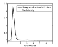
Figure 1: Normalized histogram based on a sample of the noise distribution (solid line) and the fitted density (dashed line) having the form of (21) with $\hat{\alpha}=0.961$, $\hat{\beta}=0.941$, $\hat{\nu}=5.74$, $\hat{\tau}=5.89$.

To determine the rate of convergence of the MISE, it is necessary to specify the type of the noise distribution. Here two cases are considered. First, the noise distribution can be exponential with density given by $f_{\eta}(x)=\theta e^{-\theta x}{{\mbox{$\mathds{1}$}}}_{x>0}\;,$ for some $\theta>0$. Then we have $f_{\eta}^{*}(u)=\theta/(\theta+iu)$, $|f_{\eta}^{*}(u)|^{2}=1/(1+u^{2}/\theta^{2})$ and $\Delta_{\eta}(m)=m+\pi^{2}m^{3}/(3\theta^{2})$.

In the fluorescence setting, we found that TCSPC noise distributions can be approximated by densities of the following form

$$f_{\eta}(x)=\left(\frac{\alpha\nu}{\alpha-\beta}e^{-\nu x}-\frac{\beta\tau}{\alpha-\beta}e^{-\tau x}\right){{\mbox{$\mathds{1}$}}}_{\{x>0\}}\;,$$ (21)

with constraints $\alpha>\beta$, $\nu<\tau$, $\beta\tau/(\alpha\nu)\geq 1$. Figure 1 presents a dataset with 259,260 measurements from the noise distribution of a TCSPC instrument (independently from the fluorescence measurements) and the corresponding estimated density having form (21) obtained by least squares fitting. Even though the fit is not perfect, the estimated density captures the main features of the dataset. Thus densities of the form (21) can be considered as a good approximative model of the noise distribution in the fluorescence setting. In the general case of (21) we have

$$f_{\eta}^{*}(u)=\frac{\alpha\nu}{\alpha-\beta}\frac{1}{\nu+iu}-\frac{\beta\tau}{\alpha-\beta}\frac{1}{\tau+iu}\;.$$

In the simulation study we will consider a noise distribution of the form (21) with parameters $\alpha=2,\beta=1,\nu=1$, $\tau=2$. In this case we get

$$|f_{\eta}^{*}(u)|^{2}=\frac{4}{(1+u^{2})(4+u^{2})}\qquad\text{ and }\qquad\Delta_{\eta}(m)=m+\frac{5}{12}\pi^{2}m^{3}+\frac{1}{20}\pi^{4}m^{5}\;.$$ (22)

From the application viewpoint it is hence interesting to consider the class of noise distributions $\eta$ whose characteristic functions decrease in the ordinary smooth way of order $\gamma$, denoted by $\eta\sim OS(\gamma)$, defined by $c_{0}(1+u^{2})^{-\gamma}\leq|f_{\eta}^{*}(u)|^{2}\leq C_{0}(1+u^{2})^{-\gamma}.$ Clearly, we find that $\Delta_{\eta}(m)=O(m^{2\gamma+1})$.

3.4 Rates of convergence on Sobolev spaces

In classical deconvolution the regularity spaces used for the functions to estimate are Sobolev spaces defined by

$${\mathcal{C}}(a,L)=\left\{g\in({\mathbb{L}}^{1}\cap{\mathbb{L}}^{2})({\mathbb{R}}),\;\int(1+u^{2})^{a}|g^{*}(u)|^{2}\mathrm{d}u\leq L\right\}\;.$$

If $f_{Y}$ belongs to ${\mathcal{C}}(a,L)$, then

$$\|f_{Y}-f_{Y,m}\|^{2} = \int_{|u|\geq\pi m}|f_{Y}^{*}(u)|^{2}\mathrm{d}u=\int_{|u|\geq\pi m}(1+u^{2})^{a}|f_{Y}^{*}(u)|^{2}/(1+u^{2})^{a}\mathrm{d}u$$

$$\leq (1+(\pi m)^{2})^{-a}L\leq L(\pi m)^{-2a}\;.$$

Therefore, if $f_{Y}\in{\mathcal{C}}(a,L)$ and $\eta\sim OS(\gamma)$, Proposition 3.1 implies that ${\mathbb{E}}(\|\bar{f}_{m}-f_{Y}\|^{2})\leq C_{1}m^{-2a}+C_{2}n^{-1}{m^{2\gamma+1}}.$ The optimization of this upper bound provides the optimal choice of $m$ by $m_{opt}=O(n^{1/(2a+2\gamma+1)})$ with resulting rate ${\mathbb{E}}(\|\hat{f}_{m}-f_{Y}\|^{2})\leq O(n^{-2a/(2a+2\gamma+1)})$. More formally, one can show the following result.

Proposition 3.2

Assume that the assumptions of Proposition 3.1 are satisfied and that $f_{Y}\in{\mathcal{C}}(a,L)$ and $\eta\sim OS(\gamma)$, then for $m_{opt}=O(n^{1/(2a+2\gamma+1)})$, we have

$${\mathbb{E}}(\|\bar{f}_{m_{opt}}-f_{Y}\|^{2})\leq O(n^{-2a/(2a+2\gamma+1)})\;.$$

Obviously, in practice the optimal choice $m_{opt}$ is not feasible since $a$ is and part of the constants involved in the order are unknown. Therefore, another model selection device is required to choose a relevant $\bar{f}_{m}$ in the collection.

3.5 Model selection

The general method consists in finding a data driven penalty $\overline{{\rm pen}}(.)$ such that the following model

$$\bar{m}=\arg\min_{m\in{\mathcal{M}}_{n}}(\gamma_{n}^{\dagger}(\bar{f}_{m})+\overline{{\rm pen}}(m))$$ (23)

achieves a bias-variance trade-off, where ${\mathcal{M}}_{n}$ has to be specified. In contrast to this general approach our result involves an additional $\ln(n)$-factor in the penalty compared to the variance order, which implies a loss with respect to the expected rate derived in Section 3.4.

Theorem 3.1

Assume that $f_{Y}$ is square integrable on ${\mathbb{R}}$, $\eta\sim OS(\gamma)$ and $w$ satisfies (6) and (9). Consider the estimator $\bar{f}_{\bar{m}}$ with model $\bar{m}$ defined by (23) with penalty

$$\overline{{\rm pen}}(m)=\kappa^{\prime}\left(\int_{0}^{1}w^{2}(u)\mathrm{d}u+\kappa^{\prime\prime}c_{w}^{2}\ln(n)\right)\frac{\Delta_{\eta}(m)}{n}\;,$$ (24)

where $\kappa^{\prime}$ and $\kappa^{\prime\prime}$ are numerical constants. Assume moreover that $\eta$ is ordinary smooth, i.e. $\eta\sim OS(\gamma)$, and that the model collection is described by ${\mathcal{M}}_{n}=\{m\in{\mathbb{N}},\Delta_{\eta}(m)\leq n\}=\{1,\dots,m_{n}\}$. Then, there exist constants $\kappa^{\prime},\kappa^{\prime\prime}$ such that

$${\mathbb{E}}\left(\|\bar{f}_{\bar{m}}-f_{Y}\|^{2}\right)\leq C\left(\inf_{m\in{\mathcal{M}}_{n}}\|f_{Y}-f_{Y,m}\|^{2}+\overline{{\rm pen}}(m)\right)+C^{\prime}\frac{\ln(n)}{n}\;,$$ (25)

where $C$ is a numerical constant and $C^{\prime}$ depends on $c_{w}$ and the bounds on $w$.

As previously, the numerical constants $\kappa^{\prime}$ and $\kappa^{\prime\prime}$ are calibrated via simulations. In practice, to compute $\bar{m}$ by (23), we approximate $\gamma_{n}^{\dagger}(\bar{f}_{m})$ by $-\sum_{|j|\leq K_{n}}|\bar{a}_{m,j}|^{2}$, where the sum is truncated to $K_{n}$ of order $n$.

In the fluorescence set-up, the noise distribution $f_{\eta}$ is generally unknown. However, independent, large samples of the noise distribution are available. Hence one may still use the procedure proposed above by replacing $f_{\eta}^{*}$ with the estimate $\hat{f}_{\eta}^{*}(u)=\sum_{k=1}^{n}e^{-iu\eta_{-k}}/n,$ where $(\eta_{-k})_{1\leq k\leq M}$ denotes the independent noise sample. In Comte and Lacour (2009) the same substitution is considered for deconvolution methods. It is shown that for ordinary smooth noise this leads to a risk bound exactly analogous to the one given in (25). The main constraint given in Comte and Lacour (2009) is that $M\geq n^{1+\epsilon}$, for some $\epsilon>0$. As the noise samples provided in fluorescence have huge size, this condition is certainly fulfilled in our practical examples. In the following numerical study we consider the estimator with both the exact $f_{\eta}^{*}$ and an estimated $\hat{f}^{*}_{\eta}$.

4 Numerical results for simulated and real data

In this section we first give details on the practical implementation of the estimation methods. Then a simulation study is conducted to test the performance of the methods in different settings. Finally, an application to a sample of fluorescence data shows that the estimation method gives satisfying results on real measurements.

4.1 Practical computation of estimators

In the case of no additional noise, we apply the method described in Section 2 with the trigonometric basis [T]. To determine the best model $\hat{m}$ we compute $\gamma_{n}(m)+\text{pen}(m)$ for all $m=1,\dots,[n/2]-1$. This is computationally easy as the following recursive relation can be used. We have $\gamma_{n}(0)+\text{pen}(0)=-\hat{a}_{0}^{2}+\kappa W/n,$ $\gamma_{n}(1)+\text{pen}(1)=-\hat{a}_{0}^{2}-\hat{a}_{1,1}^{2}-\hat{a}_{1,2}^{2}+\kappa 3W/n$ and $\gamma_{n}(m+1)+\text{pen}(m+1)=\gamma_{n}(m)+\text{pen}(m)-\hat{a}_{m+1,1}^{2}-\hat{a}_{m+1,2}^{2}+2\kappa W/n$, for all $m\geq 1$, where $W=\int_{0}^{1}w^{2}(u)\mathrm{d}u$. The coefficients are given by (8). Then $\hat{m}$ is the value where $\gamma_{n}(m)+\text{pen}(m)$ achieves its minimum. Finally, the estimator of $f$ is given by $\hat{f}_{\hat{m}}=\sum_{\lambda\in\Lambda_{\hat{m}}}\hat{a}_{\lambda}\varphi_{\lambda}$.

In the case of additional noise, we use the estimator proposed in Section 3 based on the sinc basis. Its computation is more intensive as no similar recursive relation holds. First one has to compute the coefficients $\bar{a}_{m,j}$ defined in (20). For $j\geq 0$ they can be approximated as follows

$$\bar{a}_{m,j} =\frac{1}{2\pi}\int\varphi_{m,j}^{*}(-u)\frac{\widehat{f^{*}_{X}}(u)}{f_{\eta}^{*}(u)}\mathrm{d}u=(-1)^{j}\frac{\sqrt{m}}{2}\int_{0}^{2}e^{i\pi jv}\frac{\widehat{f^{*}_{X}}(\pi m(v-1))}{f_{\eta}^{*}(\pi m(v-1))}\mathrm{d}v$$

$$\approx(-1)^{j}\frac{\sqrt{m}}{T}\sum_{t=0}^{T-1}e^{i2\pi jt/T}\frac{\widehat{f^{*}_{X}}(\pi m(\frac{2t}{T}-1))}{f_{\eta}^{*}(\pi m(2t/T-1))}=(-1)^{j}{\sqrt{m}}(\text{IFFT}(H))_{j}=\breve{a}_{m,j}\;,$$

where IFFT(H) is the inverse fast Fourier transform of the $T$-vector $H$ whose $t$-th entry equals $\widehat{f^{*}_{X}}(\pi m({2t}/T-1))/{f_{\eta}^{*}(\pi m(2t/T-1))}$. Similarly, for $j<0$ the coefficients $\bar{a}_{m,j}$ are approximated by $\breve{a}_{m,j}=(-1)^{j}{\sqrt{m}}(\text{IFFT}(\overline{H}))_{j}$.

The integral $\Delta_{\eta}(m)$ appearing in the penalty term $\overline{{\rm pen}}(m)$ defined in (24) is explicitly known if $f_{\eta}$ is known (see Section 3.3). In the case when we only have an estimator $\hat{f}_{\eta}$, $\Delta_{\eta}(m)$ can be approximated by a Riemann sum of the form $({m}/{S})\sum_{s=0}^{S}{|\hat{f}^{*}_{\eta}(-\pi m(1-\frac{2s}{S}))|^{-2}}$. Then the best model $\bar{m}$ is selected as the point of minimum of the criterion given in (23). Finally, we obtain the estimator $\bar{f}_{\bar{m}}=\sum_{j=-T}^{T}\breve{a}_{\bar{m},j}\varphi_{\bar{m},j}$ with the sinc functions $\varphi_{m,j}$ defined in (19).

Gamma	Exponential	Pareto	Weibull
0.0434	2.325	9.6035	81.010
Estimation with $\mu=0.01$, $n=1000$
0.0519	2.3306	9.6801	80.1796
Estimation with $\mu=0.5$, $n=1000$
0.0610	2.4329	9.7500	82.6353
Estimation with $\mu=2$, $n=1000$

Figure 2: True density and 25 estimated curves without measurement errors. Estimation with the trigonometric basis for different levels of the pile-up effect. Numbers below the figures are the MISE.

Figure 2 and 3 present the visual summary of our simulation results. We implemented the estimation methods when $f_{Y}$ has one of the following pdfs.

1. a Gamma(3, 3) p.d.f, $1/(2!3^{3})x^{2}\exp(-x/3){{\mbox{$\mathds{1}$}}}_{x>0}$, to have a benchmark with a smooth distribution,

2. an exponential pdf, $(1/3)\exp(-x/3){{\mbox{$\mathds{1}$}}}_{x>0}$,

3. a Pareto(1/4, 1, 0) pdf $(1+x/4)^{-5}{{\mbox{$\mathds{1}$}}}_{x>0}$,

4. a Weibull(1/4, 3/4) pdf $(3/4)(1/4)^{-3/4}x^{-1/4}\exp(-(4x)^{3/4}){{\mbox{$\mathds{1}$}}}_{x>0}$.

The last two densities are inspired by chemical results about fluorescence phenomena given in Berberan-Santos et al. (2005a, b).

4.2 Simulation study

Gamma	Exponential	Pareto	Weibull
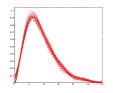
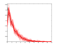
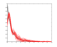
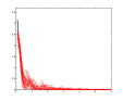
3.36 (0.49)	14.2 (2.1)	22.4 (1.8)	43.1 (5.9)
Estimation with $\sigma=0.7$, $\mu=0.01$, $n=2000$
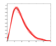
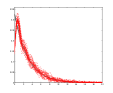
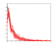
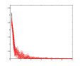
3.36 (0.57)	15.2 (1.6)	27.1 (3.6)	48.9 (6.3)
Estimation with $\sigma=0.5$, $\mu=1$, $n=2000$
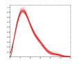
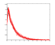
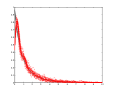
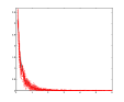
3.00 (0.00)	15.3 (2.0)	33.6 (3.5)	81.0 (7.6)
Estimation with $\sigma=0.1$, $\mu=2$, $n=2000$

Figure 3: True density and 25 estimated curves. Estimation by deconvolution with sinc basis for different noise levels and different levels of the pile-up effect. Numbers below the figures indicate mean and standard deviation of the selected model $\bar{m}$.

When no noise is added we applied the method described in Section 2 with the simple trigonometric basis. The numerical constant $\kappa$ of the penalty (14) is set to 0.5 resulting from a previous calibration by simulation. The Poisson parameter varies from 0.01 over 0.5 to 2. The mean MISE over 25 paths are computed on the intervals of representation. From Figure 2 one can see that the results are rather good, in spite of small side effects which would be avoided with piecewise polynomial bases. From this point of view all representations in Figure 2 are cut on the right. We see that the estimator performs well for a large range of values of the Poisson parameter. The first row corresponds to data where the pile-up effect is negligible, as the Poisson parameter is equal to 0.01, and hence serves as a benchmark. Here estimation errors are mainly due to the choice of a trigonometric basis, that easily recovers the Gamma density while the Weibull density is much harder to approximate in this basis. In the other rows the pile-up effect is considerably increased, however the accuracy is hardly affected and the estimator is still rather stable. The pile-up effect is hence correctly taken into account in the estimation procedure.

	Exponential noise
$(\sigma^{2},\mu)$	$(0.2,0.5)$	$(0.2,1.5)$	$(0.2,2)$	$(1,0.5)$	$(1,1.5)$	$(1,2)$
Gamma	.063 (.042)	.081 (.045)	.112 (.026)	.061 (.039)	.088 (.040)	.115 (.028)
	.063 (.042)	.081 (.045)	.112 (.026)	.061 (.039)	.087 (.040)	.115 (.028)
Exponential	1.11 (0.22)	1.20 (0.26)	1.45 (0.21)	1.36 (0.26)	1.40 (0.24)	1.67 (0.27)
	1.11 (0.22)	1.19 (0.25)	1.46 (0.21)	1.36 (0.27)	1.40 (0.24)	1.67 (0.27)
Pareto	4.25 (0.82)	4.55 (0.58)	5.45 (0.84)	6.62 (1.5)	6.58 (0.95)	8.09 (1.2)
	4.23 (0.83)	4.56 (0.61)	5.47 (0.83)	6.62 (1.6)	6.58 (1.0)	8.09 (1.2)
Weibull	10.6 (6.7)	9.46 (5.0)	9.22 (2.7)	21.4 (4.1)	26.7 (5.6)	39.5 (5.9)
	8.54 (4.7)	9.40 (4.8)	9.30 (2.3)	22.1 (4.8)	26.7 (5.7)	40.1 (5.7)
	Bi-exponential noise
$(\sigma^{2},\mu)$	$(0.2,0.5)$	$(0.2,1.5)$	$(0.2,2)$	$(1,0.5)$	$(1,1.5)$	$(1,2)$
Gamma	.060 (.032)	.075 (.040)	.113 (.023)	.061 (.048)	.088 (.043)	.114 (.025)
	.060 (.032)	.075 (.040)	.113 (.023)	.062 (.048)	.089 (.043)	.114 (.025)
Exponential	1.06 (0.20)	1.14 (0.17)	1.49 (0.26)	1.23 (0.27)	1.37 (0.28)	1.62 (0.28)
	1.06 (0.20)	1.14 (0.16)	1.48 (0.25)	1.25 (0.26)	1.37 (0.28)	1.62 (0.27)
Pareto	4.15 (0.76)	4.31 (0.69)	5.08 (0.71)	6.08 (1.5)	6.41 (1.1)	7.43 (1.0)
	4.14 (0.77)	4.30 (0.69)	5.07 (0.72)	6.11 (1.6)	6.49 (1.2)	7.45 (1.1)
Weibull	10.2 (6.1)	8.89 (5.6)	8.29 (2.1)	24.7 (3.9)	29.4 (4.5)	40.1 (5.2)
	8.25 (4.3)	8.75 (5.4)	8.31 (2.2)	24.9 (4.3)	29.5 (4.9)	40.4 (5.3)

Table 1: 100 $\times$ mean MISE and standard deviation in parentheses. First lines correspond to exact noise distribution, second lines give results obtained with estimated noise distribution.

The adaptive estimator described in Section 3 is tested with the numerical constants $\kappa^{\prime}=1$ and $\kappa^{\prime\prime}=0.001$ in (24). The value of $\kappa^{\prime\prime}$ is very small and makes the logarithmic term in general negligible except when $c_{w}^{2}$ is large (for instance $c_{w}^{2}\approx 416$ for $\mu=2$). The results are given in Figure 3. Now the observations are $Y=X+\eta$, where $\eta=\sigma\varepsilon$. In the first row, the pile-up effect is almost negligible ($\mu=0.01$), but $\sigma$ is rather large. That is, the first row illustrates the performance of the deconvolution step of the estimation procedure. In contrast, for the last row $\sigma$ is taken to be small, but the pile-up effect is significant ($\mu=2$), to see how the estimator copes with the pile-up effect. The second row is an intermediate situation, illustrating how the estimator performs when the variance of the noise and the pile-up effect are both non negligible.

The 25 curves indicate variability bands for the estimation procedure. They show that the estimator is quite stable, especially in the last rows. Moreover, the selected model order $\bar{m}$ is different from one example to the other. Globally the dimension $m$ increases when going from example 1 to 4. That means that the estimator adapts to the peaks that are more and more difficult to recover.

In Table 1 the MISE of the estimation procedure is analyzed. The table gives the empirical mean and standard deviation of the MISE obtained over 100 simulated datasets. This is done for the same four examples of distributions as above. We compare the error for the estimator using the exact noise distribution to the estimator based on an approximation of the noise distribution based on an independent noise sample of size 500. Moreover, we study the influence of the noise distribution on the estimator. Therefore, we consider, on the one hand exponential noise with variances $\sigma^{2}\in\{0.2,1\}$, and on the other hand density (21) with $\alpha=2$, $\beta=1$, $\nu=1$, $\tau=2$ (multiplied with adequate constants to have same variance $\sigma^{2}$ as for the exponential distributions).

From Table 1 it is clear that increasing the variance of the noise distribution increases the error. Furthermore, changing the type of the noise does not influence a lot the estimation procedure. Indeed, the second case (21) is just slightly less favorable than the exponential distribution. This difference is in accordance with Proposition 3.2 that holds with $\gamma=1$ for the exponential and with $\gamma=2$ for the other density. The comparison with the results based on an approximated noise distribution (second lines) reveals that there is rarely a difference between the two methods. Indeed, using an approximation of the noise does not corrupt the results, in some cases we even observe an improvement of the error. We show in Figure 4 that it is indispensable to take into account both the pile-up correction (which is omitted in (b) where $w(i/n)$ is replaced by $i/n$ ) and the deconvolution correction (which is omitted in (c) where the estimation is done with the method of Section 2 and the trigonometric basis). Thus, we conclude from these simulation results for the fluorescence setting that it is justified to use an estimate of the noise instead of the theoretical distribution.

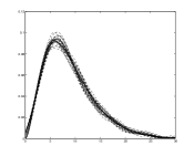
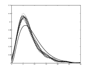
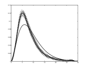
(a)                                     (b)                                     (c)

Figure 4: (a) Estimation with pile-up correction and deconvolution. (b) No pile-up correction. (c) No deconvolution.

4.3 Application to Fluorescence Measurements

We finally applied the estimation procedure to real fluorescence lifetime measurements obtained by TCSPC. The data analyzed here are graphically presented in Figure 5 (a) by the histogram of the fluorescence lifetime measurements and the histogram of the noise distribution based on a sample obtained independently from the fluorescence measurements. The sample size of the fluorescence measurements is $n=1,743,811$. The same sample of the noise distribution has already been considered in Figure 1, where it is compared to the parameterized density given by (21). In this setting the true density is known to be an exponential distribution with mean 2.54 nanoseconds and the Poisson parameter equals 0.166. The knowledge of the true density allows to evaluate the performance of our estimator. More details on the data and their acquisition can be found in Patting et al. (2007).

We applied the estimator from Section 3 with the sinc basis to this dataset. The numerical constants are $\kappa^{\prime}=1$ and $\kappa^{\prime\prime}=0.001$. Figure 5 (b) shows the estimation result in comparison to the exponential density with mean 2.54. We observe that the estimated function is quite close to the ‘true’ one. This indicates that the estimation procedure takes the errors present in the real data adequately into account and that the modeling by the pile-up distortion and additive measurement errors is appropriate.

We conclude that the estimation methods proposed in this paper have a satisfactory behavior in various settings and give rather good results on both synthetic and real data. Nevertheless, we observed that the performance depends on the choice of the basis and on the smoothness of the target density. Here only two bases are considered, but others should work as well and may improve the results in certain settings.

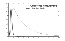
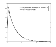
(a)                                             (b)

Figure 5: (a) Fluorescence lifetime measurements (solid line) and independent sample of the noise distribution (dashed). (b) Density estimator (solid) and ‘true’ exponential density with mean 2.54 (dashed).

5 Proofs

5.1 Proof of Proposition 2.1.

Pythagoras formula yields $\|f-\hat{f}_{m}\|^{2}=\|f-f_{m}\|^{2}+\|f_{m}-\hat{f}_{m}\|^{2}.$ By definition of the orthogonal projection $f_{m}=\sum_{\lambda\in\Lambda_{m}}a_{\lambda}\varphi_{\lambda}$ and by using equality (4), we have $a_{\lambda}=\langle\varphi_{\lambda},f_{Y}\rangle={\mathbb{E}}(\varphi_{\lambda}(Y))={\mathbb{E}}(\varphi_{\lambda}(Z_{1})w\circ G(Z_{1})).$ This, together with formula (8) implies that $\|f_{m}-\hat{f}_{m}\|^{2}=\sum_{\lambda\in\Lambda_{m}}(a_{\lambda}-\hat{a}_{\lambda})^{2}.$ If we define

$$\nu_{n}(h)=\frac{1}{n}\sum_{i=1}^{n}[h(Z_{i})w\circ G(Z_{i})-{\mathbb{E}}(h(Z_{i})~{}w\circ G(Z_{i}))],$$ (26)

$$R_{n}(h)=\frac{1}{n}\sum_{i=1}^{n}h(Z_{i})[w\circ\hat{G}_{n}(Z_{i})-w\circ G(Z_{i})]\;,$$ (27)

then we get $\|f_{m}-\hat{f}_{m}\|^{2}\leq 2\sum_{\lambda\in\Lambda_{m}}(\nu_{n}(\varphi_{\lambda})^{2}+R_{n}(\varphi_{\lambda})^{2}).$ We have, on the one hand,

$$\sum_{\lambda\in\Lambda_{m}}{\mathbb{E}}(\nu_{n}^{2}(\varphi_{\lambda}))=\sum_{\lambda\in\Lambda_{m}}\frac{1}{n}{\rm Var}(\varphi_{\lambda}(Z_{i})w\circ G(Z_{i}))\leq\sum_{\lambda\in\Lambda_{m}}\frac{1}{n}{\mathbb{E}}\left[\varphi_{\lambda}^{2}(Z_{1})(w\circ G(Z_{1}))^{2}\right]$$

$$\quad\leq\frac{1}{n}{\mathbb{E}}\left[\|\sum_{\lambda\in\Lambda_{m}}\varphi_{\lambda}^{2}\|_{\infty}(w\circ G(Z_{1}))^{2}\right]\leq\Phi_{0}\frac{D_{m}}{n}{\mathbb{E}}[(w\circ G(Z_{1}))^{2}]\leq\Phi_{0}w_{1}^{2}\frac{D_{m}}{n}\;,$$ (28)

because the basis satisfies (10). On the other hand, we have

$$\sum_{\lambda\in\Lambda_{m}}{\mathbb{E}}(R_{n}^{2}(\varphi_{\lambda}))\leq\sum_{\lambda\in\Lambda_{m}}{\mathbb{E}}\left[\left(\frac{1}{n}\sum_{i=1}^{n}\varphi_{\lambda}(Z_{i})[w\circ\hat{G}_{n}(Z_{i})-w\circ G(Z_{i})]\right)^{2}\right]$$ (29)

$$\leq \frac{1}{n}\sum_{i=1}^{n}\sum_{\lambda\in\Lambda_{m}}{\mathbb{E}}\left(\varphi_{\lambda}^{2}(Z_{i})[w\circ\hat{G}_{n}(Z_{i})-w\circ G(Z_{i})]^{2}\right)$$

$$\leq c_{w}^{2}\sum_{\lambda\in\Lambda_{m}}{\mathbb{E}}\left(\|G-\hat{G}_{n}\|_{\infty}^{2}\varphi_{\lambda}^{2}(Z_{i})\right)\leq c_{w}^{2}\Phi_{0}D_{m}{\mathbb{E}}\left(\|G-\hat{G}_{n}\|_{\infty}^{2}\right)\leq c_{w}^{2}\Phi_{0}\frac{D_{m}}{n}$$

with (9) and because of ${\mathbb{E}}\left(\|G-\hat{G}_{n}\|_{\infty}^{2}\right)\leq 1/n$ (see e.g. Brunel and Comte, 2005, p. 462). By gathering all terms, we obtain the risk bound stated in Proposition 2.1. $\Box$

5.2 Sketch of proof of Theorem 2.1

We can write $\gamma_{n}(t)-\gamma_{n}(s)=\|t-f_{Y}\|^{2}-\|s-f_{Y}\|^{2}-2\nu_{n}(t-s)-2R_{n}(t-s),$ where $\nu_{n}$ and $R_{n}$ are defined by (26) and (27). By definition of $\hat{f}_{\hat{m}}$ we have for all $m\in{\mathcal{M}}_{n}$, $\gamma_{n}(\hat{f}_{\hat{m}})+{\rm pen}(\hat{m})\leq\gamma_{n}(f_{m})+{\rm pen}(m)$. This can be rewritten as $\|\hat{f}_{\hat{m}}-f_{Y}\|^{2}\leq\|f_{m}-f_{Y}\|^{2}+{\rm pen}(m)+2\nu_{n}(\hat{f}_{\hat{m}}-f_{m})-{\rm pen}(\hat{m})+2R_{n}(\hat{f}_{\hat{m}}-f_{m}).$ Using this and and that $2xy\leq x^{2}/\theta+\theta y^{2}$ for all nonnegative $x,y,\theta$, we obtain

$$\|f_{Y}-\hat{f}_{\hat{m}}\|^{2} \leq\|f_{Y}-f_{m}\|^{2}+{\rm pen}(m)+2\nu_{n}(\hat{f}_{\hat{m}}-f_{m})-{\rm pen}(\hat{m})+2R_{n}(\hat{f}_{\hat{m}}-f_{m})$$

$$\|f_{Y}-\hat{f}_{\hat{m}}\|^{2} \leq\|f_{Y}-f_{m}\|^{2}+{\rm pen}(m)+2\|\hat{f}_{\hat{m}}-f_{m}\|\sup_{t\in S_{\hat{m}}+S_{m},\|t\|=1}|\nu_{n}(t)|-{\rm pen}(\hat{m})$$

$$+2\|\hat{f}_{\hat{m}}-f_{m}\|\sup_{t\in S_{\hat{m}}+S_{m},\|t\|=1}|R_{n}(t)|$$

$$\leq\|f_{Y}-f_{m}\|^{2}+{\rm pen}(m)+\frac{1}{4}\|\hat{f}_{\hat{m}}-f_{m}\|^{2}+2\sup_{t\in S_{\hat{m}}+S_{m},\|t\|=1}[\nu_{n}(t)]^{2}$$

$$-{\rm pen}(\hat{m})+\frac{1}{8}\|\hat{f}_{\hat{m}}-f_{m}\|^{2}+8\sup_{t\in S_{\hat{m}}+S_{m},\|t\|=1}[R_{n}(t)]^{2}\;.$$

As $\|\hat{f}_{\hat{m}}-f_{m}\|^{2}\leq 2(\|\hat{f}_{\hat{m}}-f\|^{2}+\|f_{m}-f\|^{2})$, this yields

$$\frac{1}{4}{\mathbb{E}}[\|f-\hat{f}_{\hat{m}}\|^{2}] \leq \frac{7}{4}\|f-f_{m}\|^{2}+2{\rm pen}(m)+8{\mathbb{E}}\left(\sup_{t\in S_{m_{n}},\|t\|=1}[R_{n}(t)]^{2}\right)$$

$$+4{\mathbb{E}}\left(\sup_{t\in S_{\hat{m}}+S_{m},\|t\|=1}[\nu_{n}(t)]^{2}-({\rm pen}(m)+{\rm pen}(\hat{m}))/4\right)_{+}\;.$$

Then the term ${\mathbb{E}}\left(\sup_{t\in S_{\hat{m}}+S_{m},\|t\|=1}[\nu_{n}(t)]^{2}-({\rm pen}(m)+{\rm pen}(\hat{m}))/4\right)_{+}$ is bounded by $C/n$ by using Talagrand Inequality in a standard way (see e.g. Brunel et al., 2005). For the last term ${\mathbb{E}}\left(\sup_{t\in S_{m_{n}},\|t\|=1}[R_{n}(t)]^{2}\right)$, we define $\Omega_{G}$ by

$$\Omega_{G}={\{\sqrt{n}\|\hat{G}_{n}-G\|_{\infty}\leq\sqrt{\ln(n)}\}}.$$ (30)

Now, we know from Massart (1990) that

$${\mathbb{P}}(\sqrt{n}\|\hat{G}_{n}-G\|_{\infty}\geq\lambda)\leq 2e^{-2\lambda^{2}}.$$ (31)

This implies that ${\mathbb{P}}(\Omega_{G}^{c})\leq 2/n^{2}$. Then we write that ${\mathbb{E}}\left(\sup_{t\in S_{m_{n}},\|t\|=1}[R_{n}(t)]^{2}\right)$ is less than

$${\mathbb{E}}\left(\sup_{t\in S_{m_{n}},\|t\|=1}[R_{n}(t){{\mbox{$\mathds{1}$}}}_{\Omega_{G}}]^{2}\right)+{\mathbb{E}}\left(\sup_{t\in S_{m_{n}},\|t\|=1}[R_{n}(t){{\mbox{$\mathds{1}$}}}_{\Omega_{G}^{c}}]^{2}\right) :={\mathcal{R}}_{1}+{\mathcal{R}}_{2}.$$

For the first term, we have

$${\mathcal{R}}_{1} \leq c_{w}^{2}{\mathbb{E}}\left[\|\hat{G}_{n}-G\|^{2}_{\infty}{{\mbox{$\mathds{1}$}}}_{\Omega_{G}}{\mathbb{E}}\left(\sup_{t\in S_{m_{n}},\|t\|=1}(\frac{1}{n}\sum_{i=1}^{n}|t(Z_{i})|)^{2}\right)\right]$$

$$\leq c_{w}^{2}\frac{\ln(n)}{n}{\mathbb{E}}\left(\sup_{t\in S_{m_{n}},\|t\|=1}(\frac{1}{n}\sum_{i=1}^{n}t^{2}(Z_{i}))\right)$$

$$\leq 2c_{w}^{2}\frac{\ln(n)}{n}\left[{\mathbb{E}}\left(\sup_{t\in S_{m_{n}},\|t\|=1}|\nu^{\prime}_{n}(t^{2})|\right)+\sup_{t\in S_{m_{n}},\|t\|=1}{\mathbb{E}}(t^{2}(Z_{1}))\right]$$

where $\nu^{\prime}_{n}(t)=\frac{1}{n}\sum_{i=1}^{n}(t(Z_{i})-{\mathbb{E}}(t(Z_{1}))$. It is proved in Brunel and Comte (2005) that ${\mathbb{E}}\left(\sup_{t\in S_{m_{n}},\|t\|=1}|\nu^{\prime}_{n}(t^{2})|\right)\leq C\ln(n)$ if the density of $Z_{1}$ is bounded and $N_{n}\leq O(n)$ for bases [DP] and [W] and $N_{n}\leq O(\sqrt{n})$ for basis [T]. Moreover ${\mathbb{E}}(t^{2}(Z_{1}))\leq\|t\|^{2}\|f_{Y}\|_{\infty}/w_{0}$. We obtain ${\mathcal{R}}_{1}\leq C\ln^{2}(n)/n$. On the other hand, we have

$${\mathcal{R}}_{2} \leq \sum_{\lambda}{\mathbb{E}}(R_{n}^{2}(\varphi_{\lambda}){{\mbox{$\mathds{1}$}}}_{\Omega^{c}})\leq c_{w}^{2}\Phi_{0}n{\mathbb{E}}^{1/2}(\|\hat{G}_{n}-G\|^{4}_{\infty}){\mathbb{P}}^{1/2}(\Omega_{G}^{c})\leq\frac{C}{n}.$$

This yields ${\mathbb{E}}\left(\sup_{t\in S_{m_{n}},\|t\|=1}[R_{n}(t)]^{2}\right)\leq C\ln^{2}(n)/n$. Finally we obtain that, for all $m\in{\mathcal{M}}_{n}$, ${\mathbb{E}}[\|f-\hat{f}_{\hat{m}}\|^{2}]\leq 7\|f-f_{m}\|^{2}+8{\rm pen}(m)+K{\ln^{2}(n)}/n$, which ends the proof. $\Box$

5.3 Proof of Proposition 3.1.

We have $\|\bar{f}_{m}-f_{Y}\|^{2}={(2\pi)^{-1}}\|\bar{f}_{m}^{*}-f_{Y}^{*}\|^{2}=(2\pi)^{-1}(\|\bar{f}_{m}^{*}-f_{Y,m}^{*}\|^{2}+\|f_{Y,m}^{*}-f_{Y}^{*}\|^{2}).$

$$\|\bar{f}_{m}^{*}-f_{Y,m}^{*}\|^{2}=\int_{-\pi m}^{\pi m}\frac{\mathrm{d}u}{|f_{\eta}^{*}(u)|^{2}}\frac{1}{n^{2}}\left|\sum_{k=1}^{n}\left[e^{-iuZ_{k}}w\circ\hat{G}_{n}(Z_{k})-{\mathbb{E}}(e^{-iuZ_{k}}w\circ G(Z_{k}))\right]\right|^{2}$$

$$\quad\leq 2\int_{-\pi m}^{\pi m}\frac{\mathrm{d}u}{|f_{\eta}^{*}(u)|^{2}}\frac{1}{n^{2}}\left|\sum_{k=1}^{n}\left[e^{-iuZ_{k}}w\circ\hat{G}_{n}(Z_{k})-e^{-iuZ_{k}}w\circ G(Z_{k})\right]\right|^{2}$$

$$\qquad+2\int_{-\pi m}^{\pi m}\frac{\mathrm{d}u}{|f_{\eta}^{*}(u)|^{2}}\frac{1}{n^{2}}\left|\sum_{k=1}^{n}\left[e^{-iuZ_{k}}w\circ G(Z_{k})-{\mathbb{E}}(e^{-iuZ_{k}}w\circ G(Z_{k}))\right]\right|^{2}\;.$$ (32)

The expectation of the first term on the right-hand side of (32) is less than or equal to

$$\frac{2}{n}\sum_{k=1}^{n}\int_{-\pi m}^{\pi m}\frac{\mathrm{d}u}{|f_{\eta}^{*}(u)|^{2}}{\mathbb{E}}(|w\circ\hat{G}_{n}(Z_{k})-w\circ G(Z_{k})|^{2})$$

$$\leq c_{w}^{2}{\mathbb{E}}\left(\|\hat{G}_{n}-G\|^{2}_{\infty}\right)\int_{-\pi m}^{\pi m}\mathrm{d}u/|f_{\eta}^{*}(u)|^{2}\leq 2\pi c_{1}c_{w}^{2}\frac{\Delta_{\eta}(m)}{n}\;,$$

by using ${\mathbb{E}}(\|\hat{G}_{n}-G\|^{2k}_{\infty})\leq c_{k}/n^{k}$ (see e.g. Lemma 6.1 p. 462, Brunel and Comte (2005) which is a straightforward consequence of Massart (1990)). Here $c_{k}$ is a numerical constant that depends on $k$ only. The expectation of the second term on the right-hand side of (32) is a variance and less than or equal to

$$\frac{2}{n}\int_{-\pi m}^{\pi m}\frac{\mathrm{d}u}{|f_{\eta}^{*}(u)|^{2}}{\rm Var}(e^{-iuZ_{1}}w\circ G(Z_{1}))\leq 4\pi\frac{\Delta_{\eta}(m){\mathbb{E}}[(w\circ G(Z_{1}))^{2}]}{n}\;.$$

Gathering the terms completes the proof of Proposition 3.1. $\Box$

5.4 Proof of Theorem 3.1.

We have the following decomposition of the contrast for functions $s,t$ in $\bar{S}_{m}$,

$$\gamma_{n}^{\dagger}(t)-\gamma_{n}^{\dagger}(s)=\|t-f_{Y}\|^{2}-\|s-f_{Y}\|^{2}-2\bar{\nu}_{n}(t-s)-2\bar{R}_{n}(t-s)\;,$$ (33)

where

$$\bar{\nu}_{n}(t)=\frac{1}{2\pi n}\sum_{k=1}^{n}\int\frac{t^{*}(-u)\left[e^{-iuZ_{k}}(w\circ G)(Z_{k})-{\mathbb{E}}(e^{-iuZ_{k}}(w\circ G)(Z_{k}))\right]}{f_{\eta}^{*}(u)}\mathrm{d}u\;,$$ (34)

and

$$\bar{R}_{n}(t)=\frac{1}{2\pi n}\sum_{k=1}^{n}\int\frac{t^{*}(-u)e^{-iuZ_{k}}}{f_{\eta}^{*}(u)}\mathrm{d}u\;[(w\circ\hat{G}_{n})(Z_{k})-(w\circ G)(Z_{k})]\;.$$ (35)

We start with decomposition (33). We take $t=\bar{f}_{\bar{m}}$ and $s=f_{Y,m}$. Since $\gamma_{n}^{\dagger}(\bar{f}_{\bar{m}})+\overline{{\rm pen}}(\bar{m})\leq\gamma_{n}^{\dagger}(f_{m})+\overline{{\rm pen}}(m)$, we get

$$\frac{1}{4}{\mathbb{E}}[\|f_{Y}-\bar{f}_{\bar{m}}\|^{2}] \leq \frac{7}{4}\|f_{Y}-f_{Y,m}\|^{2}+\overline{{\rm pen}}(m)+4{\mathbb{E}}\left(\sup_{t\in B_{m,\bar{m}}}[\bar{\nu}_{n}(t)]^{2}\right)-{\mathbb{E}}(\overline{{\rm pen}}(\bar{m}))$$ (36)

$$\hskip 28.45274pt+8{\mathbb{E}}\left(\sup_{t\in B_{m,\bar{m}}}[\bar{R}_{n}(t)]^{2}\right),$$

where $\bar{\nu}_{n}(t)$ and $\bar{R}_{n}(t)$ are defined by (34) and (35) and $B_{m}=\{t\in\bar{S}_{m},\|t\|=1\},$ and $B_{m,m^{\prime}}=\{t\in\bar{S}_{m}+\bar{S}_{m^{\prime}},\|t\|=1\}.$ Following a classical application of Talagrand Inequality in the deconvolution context for ordinary smooth noise (Comte et al., 2006), we deduce the following Lemma.

Lemma 5.1

Under the Assumptions of Theorem 3.1,

$${\mathbb{E}}\left(\sup_{t\in B_{m,\bar{m}}}[\bar{\nu}_{n}(t)]^{2}-p_{1}(m,\bar{m})\right)_{+}\leq\frac{c}{n},$$

where $p_{1}(m,m^{\prime})=2{\mathbb{E}}((w\circ G)^{2}(Z_{1}))\Delta_{\eta}(m\vee m^{\prime})/n=2(\int_{0}^{1}w^{2}(u)\mathrm{d}u)\Delta_{\eta}(m\vee m^{\prime})/n.$

Moreover for the study $\bar{R}_{n}(t)$ we have the following Lemma.

Lemma 5.2

Under the assumptions of Theorem 3.1,

$${\mathbb{E}}\left(\sup_{t\in B_{m,\bar{m}}}[\bar{R}_{n}(t)]^{2}-p_{2}(m,\bar{m})\right)\leq 0,$$

where $p_{2}(m,m^{\prime})=c_{w}^{2}\Delta_{\eta}(m\vee m^{\prime})\ln(n)/n$.

It follows from the definition of $p_{i}(m,m^{\prime})$, $i=1,2$, that there exist numerical constants $\kappa^{\prime}$ and $\kappa^{\prime\prime}$, namely $\kappa^{\prime},\kappa^{\prime\prime}\geq 8$, such that $4p_{1}(m,m^{\prime})+8p_{2}(m,m^{\prime})\leq\overline{{\rm pen}}(m)+\overline{{\rm pen}}(m^{\prime})$.

Now, starting from (36), we get, by applying Lemmas 5.1 and 5.2,

$$\frac{1}{4}{\mathbb{E}}[\|f_{Y}-\bar{f}_{\bar{m}}\|^{2}]\leq\frac{7}{4}\|f_{Y}-f_{Y,m}\|^{2}+\overline{{\rm pen}}(m)+4{\mathbb{E}}\left(\sup_{t\in B_{m,\bar{m}}}[\bar{\nu}_{n}(t)]^{2}-p_{1}(m,\bar{m})\right)_{+}$$

$$\qquad+8{\mathbb{E}}\left(\sup_{t\in B_{m,\bar{m}}}[\bar{R}_{n}(t)]^{2}-p_{2}(m,\bar{m})\right)+{\mathbb{E}}[4p_{1}(m,\bar{m})+8p_{2}(m,\bar{m})-\overline{{\rm pen}}(\bar{m})]$$

$$\quad\leq\frac{7}{4}\|f_{Y}-f_{Y,m}\|^{2}+2\overline{{\rm pen}}(m)+\frac{c}{n}.$$

Therefore if $\kappa\geq 16$, we get $(1/4){\mathbb{E}}[\|f_{Y}-\bar{f}_{\bar{m}}\|^{2}]\leq(7/4)\|f_{Y}-f_{Y,m}\|^{2}+2\overline{{\rm pen}}(m)+c/n.$ This completes the proof of Theorem 3.1. $\Box$

Proof of Lemma 5.2. First we remark that, with Cauchy-Schwarz inequality, we have

$$|\bar{R}_{n}(t)|^{2} \leq \frac{1}{4\pi^{2}}\left|\int\frac{t^{*}(-u)}{f_{\eta}^{*}(u)}\left(\frac{1}{n}\sum_{k=1}^{n}e^{-iuZ_{k}}[(w\circ\hat{G}_{n})(Z_{k})-(w\circ G)(Z_{k})]\mathrm{d}u\right)\right|^{2}$$

$$\leq \frac{1}{4\pi^{2}}\int|t^{*}(u)|^{2}\mathrm{d}u\int_{-\pi m\vee\bar{m}}^{\pi m\vee\bar{m}}\frac{\mathrm{d}u}{|f_{\eta}^{*}(u)|^{2}}\left(\frac{1}{n}\sum_{k=1}^{n}|(w\circ\hat{G}_{n})(Z_{k})-(w\circ G)(Z_{k})|^{2}\right).$$

Then Parseval Formula gives $\|t^{*}\|^{2}=2\pi\|t\|^{2}$ and we find

$$\sup_{t\in B_{m,\bar{m}}}|\bar{R}_{n}(t)|^{2}\leq c_{w}^{2}\Delta_{\eta}(m\vee\bar{m})\left(\frac{1}{n}\sum_{k=1}^{n}|\hat{G}_{n}(Z_{k})-G(Z_{k})|^{2}\right)\leq c_{w}^{2}\Delta_{\eta}(m\vee\bar{m})\|\hat{G}_{n}-\hat{G}\|_{\infty}^{2}.$$

Now, we write $\sup_{t\in B_{m,\bar{m}}}|\bar{R}_{n}(t)|^{2}={\mathcal{R}}_{1}+{\mathcal{R}}_{2}$ by inserting again the indicator functions ${{\mbox{$\mathds{1}$}}}_{\Omega_{G}}$ and ${{\mbox{$\mathds{1}$}}}_{\Omega_{G}^{c}}$ where $\Omega_{G}$ is defined by (30). Therefore

$${\mathbb{E}}\left(\sup_{t\in B_{m,\bar{m}}}[\bar{R}_{n}(t)]^{2}-p_{2}(m,\bar{m})\right)\leq{\mathbb{E}}({\mathcal{R}}_{1}-p_{2}(m,\bar{m}))+{\mathbb{E}}({\mathcal{R}}_{2})$$

$$\qquad\leq c_{w}^{2}{\mathbb{E}}\left(\Delta_{\eta}(m\vee\bar{m})(\|\hat{G}_{n}-\hat{G}\|_{\infty}^{2}{{\mbox{$\mathds{1}$}}}_{\Omega_{G}}-\frac{\ln(n)}{n})\right)$$ (37)

$$\qquad\quad+cw^{2}\Delta_{\eta}(m_{n}){\mathbb{E}}(\|\hat{G}_{n}-G\|_{\infty}^{2}{{\mbox{$\mathds{1}$}}}_{\Omega_{G}^{c}}).$$

Next $(\|\hat{G}_{n}-\hat{G}\|_{\infty}^{2}{{\mbox{$\mathds{1}$}}}_{\Omega_{G}}-\ln(n)/n))\leq 0$ by definition of $\Omega_{G}$ for the first right-hand-side term of (37). For the second term, $\Delta(m_{n})\leq n$ by the definition of $m_{n}$, $\|\hat{G}_{n}-G\|_{\infty}\leq 1$ and it follows from (31) that ${\mathbb{P}}(\Omega_{G}^{c})\leq 2/n^{2}$. Therefore

$${\mathbb{E}}\left(\sup_{t\in B_{m,\bar{m}}}[\bar{R}_{n}(t)]^{2}-p_{2}(m,\bar{m})\right)\leq c_{w}^{2}n{\mathbb{P}}(\Omega_{G}^{c})\leq 2c_{w}^{2}/n.$$

Gathering the bounds gives the result of Lemma 5.2. $\Box$

References

- Barron et al. (1999) Barron, A., Birgé, L., and Massart, P. (1999), “Risk bounds for model selection via penalization,” Probability Theory and Related Fields, 113, 301–413.
- Berberan-Santos et al. (2005a) Berberan-Santos, M. N., Bodunov, E. N., and Valeur, B. (2005a), “Mathematical functions for the analysis of luminescence decays with underlying distributions 1. Kohlrausch decay function (stretched exponential),” Chemical Physics, 515, 171–182.
- Berberan-Santos et al. (2005b) Berberan-Santos, M. N., Bodunov, E. N., and Valeur, B. (2005b), “Mathematical functions for the analysis of luminescence decays with underlying distributions: 2. Becquerel (compressed hyperbola) and related decay functions,” Chemical Physics, 317, 57–62.
- Birgé and Massart (1997) Birgé, L. and Massart, P. (1997), “From model selection to adaptive estimation,” in Festschrift for Lucien Le Cam, pp. 55–87, Springer, New York.
- Brunel and Comte (2005) Brunel, E. and Comte, F. (2005), “Penalized contrast estimation of density and hazard rate with censored data,” Sankhya, 67, 441–475.
- Brunel et al. (2005) Brunel, E., Comte, F., and Guilloux, A. (2005), “Nonparametric density estimation in presence of bias and censoring,” Test, 18, 166–194.
- Comte and Lacour (2009) Comte, F. and Lacour, C. (2009), “Data driven density estimation in presence of unknown convolution operator,” preprint available at http://www.math-info.univ-paris5.fr/map5/Prepublications-2008.
- Comte et al. (2006) Comte, F., Rozenholc, Y., and Taupin, M.-L. (2006), “Penalized contrast estimator for adaptive density deconvolution,” Canadian Journal of Statistics, 34, 431–452.
- Daubechies (1992) Daubechies, I. (1992), “Ten lectures on wavelets,” in CBMS-NSF Regional Conference Series in Applied Mathematics, Philadelphia, PA, Society for Industrial and Applied Mathematics (SIAM).
- Donoho et al. (1996) Donoho, D. L., Johnstone, I. M., Kerkyacharian, G., and Picard, D. (1996), “Density estimation by wavelet thresholding,” Annals of Statistics, 24, 508–539.
- Lakowicz (1999) Lakowicz, J. R. (1999), Principles of Fluorescence Spectroscopy, Academic/Plenum, New York.
- Massart (1990) Massart, P. (1990), “The tight constant in the Dvoretzky-Kiefer-Wolfowitz inequality,” Annals of Probability, 18, 1269–1283.
- Meyer (1990) Meyer, Y. (1990), Ondelettes et opérateurs, Hermann, Paris.
- O’Connor and Phillips (1984) O’Connor, D. V. and Phillips, D. (1984), Time-correlated single photon counting, Academic Press, London.
- Patting et al. (2007) Patting, M., Wahl, M., Kapusta, P., and Erdmann, R. (2007), “Dead-time effects in TCSPC data analysis,” in Proceedings of SPIE, vol. 6583.
- Rebafka et al. (2010) Rebafka, T., Roueff, F., and Souloumiac, A. (2010), “A corrected likelihood approach for the pile-up model with application to fluorescence lifetime measurements using exponential mixtures,” The International Journal of Biostatistics, 6.
- Rebafka et al. (2011) Rebafka, T., Roueff, F., and Souloumiac, A. (2011), “Information bounds and MCMC parameter estimation for the pile-up model,” Journal of Statistical Planning and Inference, 141, 1–16.
- Tsodikov (2003) Tsodikov, A. (2003), “A Generalized Self-Consistency Approach,” Journal of the Royal Statistical Society. Series B (Statistical Methodology), 65, 759–774.
- Valeur (2002) Valeur, B. (2002), Molecular Fluorescence, Wiley-VCH, Weinheim.