The deepest HST Color-Magnitude Diagram of M32: Evidence for Intermediate-Age Populations

Abstract

We present the deepest optical color-magnitude diagram (CMD) to date of the local elliptical galaxy M32. We have obtained $F435W$ and $F555W$ photometry based on Hubble Space Telescope ACS/HRC images for a region $110\arcsec$ from the center of M32 (F1) and a background field (F2) about $320\arcsec$ away from M32 center. Due to the high resolution of our Nyquist-sampled images, the small photometric errors, and the depth of our data (the color-magnitude diagram of M32 goes as deep as $F435W\sim 28.5$ at 50% completeness level) we obtain the most detailed resolved photometric study of M32 yet. Deconvolution of HST images proves to be superior than other standard methods to derive stellar photometry on extremely crowded HST images, as its photometric errors are $\sim 2\times$ smaller than other methods tried.

The location of the strong red clump in the CMD suggests a mean age between 8 and 10 Gyr for $[\mathrm{Fe/H}]=-0.2$ dex in M32. We detect for the first time a red giant branch bump and an asymptotic giant branch bump in M32 which, together with the red clump, allow us to constrain the age and metallicity of the dominant population in this region of M32. These features indicate that the mean age of M32’s population at $\sim 2\arcmin$ from its center is between 5 and 10 Gyr. We see evidence of an intermediate-age population in M32 mainly due to the presence of asymptotic giant branch stars rising to $\mathrm{M}_{F555W}\sim-2.0$. Our detection of a blue component of stars (blue plume) may indicate for the first time the presence of a young stellar population, with ages of the order of 0.5 Gyr, in our M32 field. However, it is likely that the brighter stars of this blue plume belong to the disk of M31 rather than to M32. The fainter stars populating the blue plume indicate the presence of stars not younger than 1 Gyr and/or blue straggler stars in M32. The CMD of M32 displays a wide color distribution of red giant branch stars indicating an intrinsic spread in metallicity with a peak at $[\mathrm{Fe/H}]\sim-0.2$. There is not a noticeable presence of blue horizontal branch stars, suggesting that an ancient population with $[\mathrm{Fe/H}]<-1.3$ does not significantly contribute to the light or mass of M32 in our observed fields. M32’s dominant population of 8–10 Gyr implies a formation redshift of $1\lesssim z_{f}\lesssim 2$, precisely when observations of the specific star formation rates and models of “downsizing” imply galaxies of M32’s mass ought to be forming their stars. Our CMD therefore provides a “ground-truth” of downsizing scenarios at $z=0$.

Our background field data represent the deepest optical observations yet of the inner disk and bulge of M31. Its CMD exhibits a broad color spread of red giant stars indicative of its metallicity range with a peak at $[\mathrm{Fe/H}]\sim-0.4$ dex, slightly more metal-poor than M32 in our fields. The observed blue plume consists of stars as young as 0.3 Gyr, in agreement with previous works on the disk of M31. The detection of bright AGB stars reveals the presence of intermediate-age population in M31, which is however less significant than that in M32 at our field’s location.

1. Introduction

Elliptical galaxies contain the oldest stars in the Universe, and the study of their composition provides a means of studying the evolution of the Universe to large look-back times. Moreover, they represent at least 50% of the total stellar mass in the local Universe (Schechter & Dressler, 1987; Gallazzi et al., 2008). Understanding their formation and evolution is crucial to understand galaxy formation and evolution in general.

The study of the resolved stellar content in galaxies is a key tool to reach this goal. Stars have the imprint of evolutionary parameters such as age and metallicity and thus provide a fossil record of the star formation history (SFH) and evolution of a galaxy. We can derive the complete SFH of a galaxy by means of deep and accurate color-magnitude diagrams (CMDs), given that the most direct information about any stellar population comes from applying stellar evolution theory to CMDs. Specifically, the direct observation of the oldest galaxy’s main-sequence turnoff (MSTO) is necessary for an accurate determination of its age and thus its SFH. Thanks to the capabilities of the Hubble Space Telescope (HST), launched in 1990, stellar populations in spirals and dwarf galaxies in the Local Group can now be resolved with great accuracy, allowing a precise determination of complete SFHs with an age resolution of $\sim 1$ Gyr for ages larger than 10 Gyr (see e.g., Brown et al., 2006; Barker et al., 2007; Cole & The Lcid Team, 2007). Unfortunately, the large distances to giant ellipticals, in combination with their high surface brightnesses, prevents detection of their intrinsically fainter individual stars, limiting knowledge about their stellar populations (although there have been studies of the resolved giants near the tip of the red giant branch in nearby ellipticals: see, e.g., Sakai et al. 1997; Harris et al. 1999; Gregg et al. 2004; Rejkuba et al. 2005). As a consequence, most elliptical galaxies can only be studied by the spectra of their integrated light which possess contributions from all their stars, having a range of metallicities and ages. This makes the unambiguous disentanglement of the age and metallicity of a stellar population difficult, especially in old populations such as those that dominate the masses of elliptical galaxies. Stellar population models have been developed to derive SFH of ellipticals (e.g. Worthey, 1994; Rose, 1994) based on moderate-resolution spectra (e.g. González, 1993; Coelho et al., 2009). These models have become very sophisticated in disentangling the non-trivial age and metallicity degeneracy. However, they still suffer several uncertainties and there is a pressing need for them to be tested with direct observations of stars in an elliptical galaxy.

1.1. M32: A window on the stellar populations of elliptical galaxies

The Local Group galaxy Messier 32 (M32) is a small satellite of M31 and the nearest elliptical galaxy. It is classified as a compact elliptical (cE) galaxy, cE2, due to its low luminosity, compactness and high surface brightness (Bender et al., 1992). M32 is the prototype of this class of ellipticals, consisting of $\sim 20$ galaxies known so far (Davidge, 1991; Ziegler & Bender, 1998; Chilingarian et al., 2009), the so-called M32-like galaxies. Despite the fact that M32 has been extensively observed and studied, its SFH and therefore its origins are still a matter of debate. The proposed models for M32’s origins span a wide range of hypotheses: from a true elliptical galaxy at the lower extreme of the mass sequence (e.g., Faber, 1973; Nieto & Prugniel, 1987; Kormendy et al., 2009) to an early-type spiral galaxy whose concentrated bulge, unlike its disk, still survives to the tidal stripping process caused by its interactions with M31 (e.g., Bekki et al., 2001; Chilingarian et al., 2009).

Nevertheless, M32 is today an elliptical galaxy and the nearest system that has properties very similar to the giant ellipticals: it falls at the lower luminosity end of all of the structural and spectroscopy scaling relations of giant ellipticals: the Faber–Jackson relation (e.g., Faber & Jackson, 1976), the Kormendy relation (e.g., Kormendy, 1985), the mass–age–metallicity and $[\alpha/\mathrm{Fe}]$–mass relationships (Trager et al., 2000a), and the Mg–$\sigma$ relation and the Fundamental Plane of early-type galaxies (e.g., Bender et al., 1992). More recently, Kormendy et al. (2009) find that both central and global parameter correlations from recent accurate photometry of galaxies in the Virgo cluster place M32 as a normal, low-luminosity elliptical galaxy in all regards.

Given its proximity, M32 provides a unique window on the stellar composition of elliptical galaxies, since it can be studied by both its integrated spectrum and the photometry of its resolved stars. While we note that the SFH of a low luminosity elliptical such as M32 ($r_{\mathrm{eff}}\approx 40\arcsec$, Choi et al. 2002; Kormendy et al. 2009) may differ from those of giant ellipticals, it is a fact that in general models applied to giant ellipticals reach the same conclusions as those applied to M32 (e.g., Worthey, 1998). M32 is therefore a vital laboratory to test the applicability of the stellar population models to more distant galaxies.

1.2. Integrated light studies of M32

From spectroscopic studies, one of the most important results of synthetic population models was found by O’Connell (1980): models fail to reproduce M32 with a single old-age and solar-metallicity population. Various synthetic population models have claimed that M32 underwent a period of significant star formation in the recent past, i.e. about 5–8 Gyr ago, (e.g., O’Connell, 1980; Pickles, 1985; Bica et al., 1990) based on the presence of enhanced H$\beta$ absorption in the integrated spectrum of M32, and thus indicate signatures of an intermediate luminosity-weighted age population (e.g., Rose, 1994; Trager et al., 2000a; Worthey, 2004; Schiavon et al., 2004; Rose et al., 2005; Coelho et al., 2009). Rose et al. (2005) studied the nuclear spectrum of M32 and found radial gradients in both the age and metallicity of the light-weighted mean stellar population of M32: the population at $1r_{\mathrm{eff}}$ is $\sim 3$ Gyr older and more metal poor by $\sim-0.25$ dex than the central population, which has a luminosity-weighted age of $\sim$ 4 Gyr and [Fe/H]$\sim 0.0$. Extrapolation of the spatially resolved spectroscopy of González (1993) results in an average age and metallicity of M32 at 1$\arcmin$ from its center of 8 Gyr old and [Fe/H]$\sim-0.25$ (Trager et al., 2000a). This is consistent with a more recent estimate by Worthey (2004) who found the age of M32 at 1$\arcmin$ to be 10 Gyr old. The most recent results from stellar population models are given by Coelho et al. (2009) who observed high signal-to-noise spectra at three different radii, from the nucleus of M32 out to $\sim 2\arcmin$ from the center of M32. They propose that an ancient and intermediate-age populations are both present in M32 and that the contribution from the intermediate population is larger at the nuclear region. They claim that a young population is present at all radii (see also e.g., Trager et al., 2000a; Rose, 1985, 1994; Schiavon et al., 2004), but its origin is unclear. Moreover, the determination of ages in integrated spectra is a difficult problem, as extended horizontal branch morphologies and/or blue stragglers, unaccounted for in the models, can mimic younger ages (e.g., Burstein et al., 1984; Rose, 1985; de Freitas Pacheco & Barbuy, 1995; Maraston & Thomas, 2000; Trager et al., 2005). Thus, lacking any direct evidence for such a young population (ages $<1$ Gyr), and due to the uncertainties in the synthesis models, these results should be considered with some caution.

1.3. Individual stars studies of M32

On the other hand, photometric studies of resolved stars have supported the existence of an intermediate-age population (e.g. Freedman, 1992a; Davidge & Jensen, 2007) by detecting AGB stars suggestive of a $\sim$ 3 Gyr old population. However, observations by Davidge & Jensen (2007), obtained with the NIRI imager on the Gemini North telescope, do not support spectroscopic studies that find an age gradient in M32, since they suggest that the AGB stars and their progenitors are smoothly mixed throughout the main body of the galaxy. Brown et al. (2000, 2008), using ultraviolet observations of the center of M32, and Fiorentino et al. (2010), using the ACS/HRC data presented here, have found evidence of an ancient, metal-poor population by observing blue horizontal branch and RR Lyrae stars, respectively. Worthey et al. (2004), using optical observations obtained with the Wide Field Planetary Camera 2 (WFPC2) on board HST and presented by Alonso-García et al. (2004), studied the stellar populations of the outer regions of M32 and M31 and found that there is no trace of a main sequence younger than $\sim 1$ Gyr in M32 at a region $7r_{\mathrm{eff}}$ from its center. The most extensive study of the resolved stellar populations of M32 has been carried out by Grillmair et al. (1996, hereafter G96), who resolved individual stars down to slightly below the level of the HB with the HST WFPC2 in a region of 1–$2\arcmin$ from the center of the galaxy. Their most important result is the composite nature of the CMD of M32. They concluded that the wide spread in color of the giant stars in their CMD cannot be explained only by a spread in age but rather by a wide spread in metallicity. However, given the age–metallicity degeneracy on the giant branch, there may well be a mixture of ages present in their field, but age effects are less important than metallicity on the giant branch morphology. For an assumed age of 8.5 Gyr old, the metallicity distribution function has a peak at $\mathrm{[Fe/H]}\sim-0.25$, consistent with the extrapolation made from the spatially resolved spectroscopy of González (1993). The spread in metallicity found by G96 ranges from roughly solar to below $-1$ dex. This study, as well as those by Brown et al., Alonso-Garcia et al. and Worthey et al., concluded that the metal-poor population is insignificant, contrary to the results of Coelho et al. (2009). Finally, a young population of $\lesssim 1$ Gyr claimed by several population models to be present in the spectrum of M32 has not been seen by any of the observations of resolved stars. Overall, the photometric studies carried out so far only obtained information from the brighter stars of M32, i.e., the upper CMD. These studies were prevented from observing fainter stars by the extreme crowding of M32. Since upper giant-branch tracks are degenerate in age and metallicity, much like integrated colors and metallic lines, it is not possible to derive an age from the upper CMD alone.

The only way to derive the SFH of M32 and test conclusions so far based solely on integrated colors and spectral indices is to obtain deep CMDs that reach the MSTO of M32. Measuring the position of the blue turnoff stars with accurate photometry is the only evidence to test the ages inferred from population synthesis models. A deep CMD and luminosity function of M32 can be used as the basis for spectral synthesis studies. An agreement between observed and synthetic indices for M32 would confirm such indices as simple diagnostic tools for constraining stellar populations in integrated light of other elliptical galaxies, for which only the integrated light is available, given their greater distances. Moreover the CMD allows for the study of spreads about mean properties in a way that is currently impossible with integrated light. These spreads are as important as the mean values in decoding the SFH of the galaxy.

In order to further investigate the stellar content of M32, and with the primary goal of deriving a complete SFH of this enigmatic galaxy, we were awarded 64 orbits of the HST to observe the MSTO of M32 with the High-Resolution Channel (HRC) at the Advanced Camera for Surveys (ACS). The proximity of M32, combined with the high resolution of HST ACS/HRC allows for a remarkable improvement in our study of its stellar content. In this paper, we introduce our new observations and present the deepest optical CMD so far obtained. The CMD presented here reaches more than 2 magnitudes fainter than the previous optical CMD by G96 and fully resolves the red giant branch (RGB) and the asymptotic giant branch (AGB). We report the discovery of a blue plume (BP), consisting of young stars and/or blue straggler stars, not claimed to have been observed before. We also detect for the first time in M32 a RGB bump and an AGB bump. By analyzing our CMD we have achieved the most comprehensive photometric study of the resolved stellar content of M32. A follow-up paper will present the recent and intermediate SFH of M32 that can be derived from these data. In addition, as discussed above, these data have already been analyzed by Fiorentino et al. (2010, hereafter F10) to study RR Lyrae variables in our fields.

The paper is organized as follows. Section 2 describes our observations and the reduction of the data. The photometry performed and the extensive study of completeness and crowding of the data are presented in Section 3. Section 4 presents the decontamination of the M32 field from the light contribution by M31. The analysis of the CMD of M32 and its luminosity function is presented in Section 5. We derive the distance to M32 and M31 is Section 6. In Section 7 we analyze the M31 stellar populations in our background field. We summarize our findings in Section 8.

2. Observations and Data reduction

2.1. Field Selection and Observational Strategy

We obtained deep $B$ and $V$-band imaging of two fields near M32 using the ACS/HRC instrument on board HST during Cycle 14 (Program GO-10572, PI: Lauer). The ACS $F435W$ ($B$) and $F555W$ ($V$) filters were selected to optimize detection of MSTO stars over the redder and more luminous stars of the giant branch. M32 is very compact and is projected against the disk of M31. The major challenge was to select a field that represented the best compromise between the extreme crowding in M32, which would drive the field to be placed as far away from the center of the galaxy as possible, versus maximizing the contrast of M32 against the M31 background populations, which would push the field back towards the central, bright portions of M32. Following these constraints, the M32 HRC field (designated F1) was centered on a location $110^{\prime\prime}$ south (the anti-M31 direction) of the M32 nucleus, roughly on the major axis of the galaxy. The $V$-band surface brightness of M32 near the center of the field is $\mu_{V}\approx 21.9$ (Kormendy et al., 2009). M32 quickly becomes too crowded to resolve faint stars at radii closer to the center, while the galaxy rapidly falls below the M31 background at larger radii.

Even at the location of F1, M31 contributes $\sim 1/3$ of the total light with inner disk and bulge stars (K. Howley, private comm.), thus it was critical to obtain a background field, F2, at the same isophotal level in M31 ($\mu_{V}\approx 22.7$) to allow for the strong M31 contamination to be subtracted from the analysis of the M32 stellar population. F2, which also contains both inner disk and bulge M31 stars (K. Howley, private comm.), was located $327^{\prime\prime}$ from the M32 nucleus at position angle $65^{\circ}$. At this angular distance M32 has an ellipticity of $\epsilon\approx 0.25$ (Choi et al., 2002) and F2 is nearly aligned with M32’s minor axis. Thus the implied semi-major axis of the M32 isophote that passes through F2 is $435^{\prime\prime},$ significantly larger than the nominal angular separation. The estimated M32 surface brightness at F2 is $\mu_{V}\approx 27.5,$ based on a modest extrapolation of the $B$-band surface photometry of Choi et al. (2002) and an assumed color of $B-V\approx 0.9$. The contribution of M32 to F2 thus falls by a factor of $\sim 180$ relative to its surface brightness at F1. While one might have been tempted to move F2 even further away from F1, it clearly serves as an adequate background at the location selected, while uncertainties in the M31 background would increase at larger angular offsets. The locations of both fields are shown in Figure 1.

Table 1Log of observations

Field	$\alpha_{J2000.0}$	$\delta_{J2000.0}$	Filter	Exposure time (s)	Date	FWHM ($\arcsec$)
F1	00 42 47.63	+40 50 27.40	$F435W$	16$\times$1279 + 16$\times$1320	Sept 20–22, 2005	0.04
F1	00 42 47.63	+40 50 27.40	$F555W$	16$\times$1279 + 16$\times$1320	Sept 22–24, 2005	0.05
F2	00 43 07.89	+40 54 14.50	$F435W$	16$\times$1279 + 16$\times$1320	Feb 6–8, 2006	0.04
F2	00 43 07.89	+40 54 14.50	$F555W$	16$\times$1279 + 16$\times$1320	Feb 9–12, 2006	0.05

Detection of the MSTO required deep exposures at F1. Accurate treatment of the background required equally deep exposures to be obtained in F2. A summary of the observations is shown in in Table 1; briefly, each field was observed for 16 orbits in each of the $F435W$ and $F555W$ filters for a total program of 64 orbits.

At $B$, and even $V$, HRC undersamples the PSF, despite its exceptionally fine pixel scale. All of the images were obtained in a $0.5\times 0.5$ sub-pixel square dither pattern to obtain Nyquist sampling in the complete data set. In detail, the sub-pixel dither pattern was executed across each pair of orbits, with each orbit split into two sub-exposures. The telescope was then offset by $0\farcs 125$ steps between the orbit pairs in a “square-spiral” dither pattern of maximum extent $\pm 5$ pixels to minimize the effects of “hot pixels,” bad columns, and any other fixed-defects in the CCD, on the photometry at any location. The data for each filter/field combination thus comprises 8 slightly different pointings, with Nyquist-sampling obtained at each location.

In addition to the HRC images, parallel observations were obtained with the ACS/WFC channel using the $F606W$ filter (broad $V$). Those images have been analyzed by Sarajedini et al. (2009), who find 324 and 357 RR Lyrae variables stars in the parallel fields associated with F1 and F2, respectively.

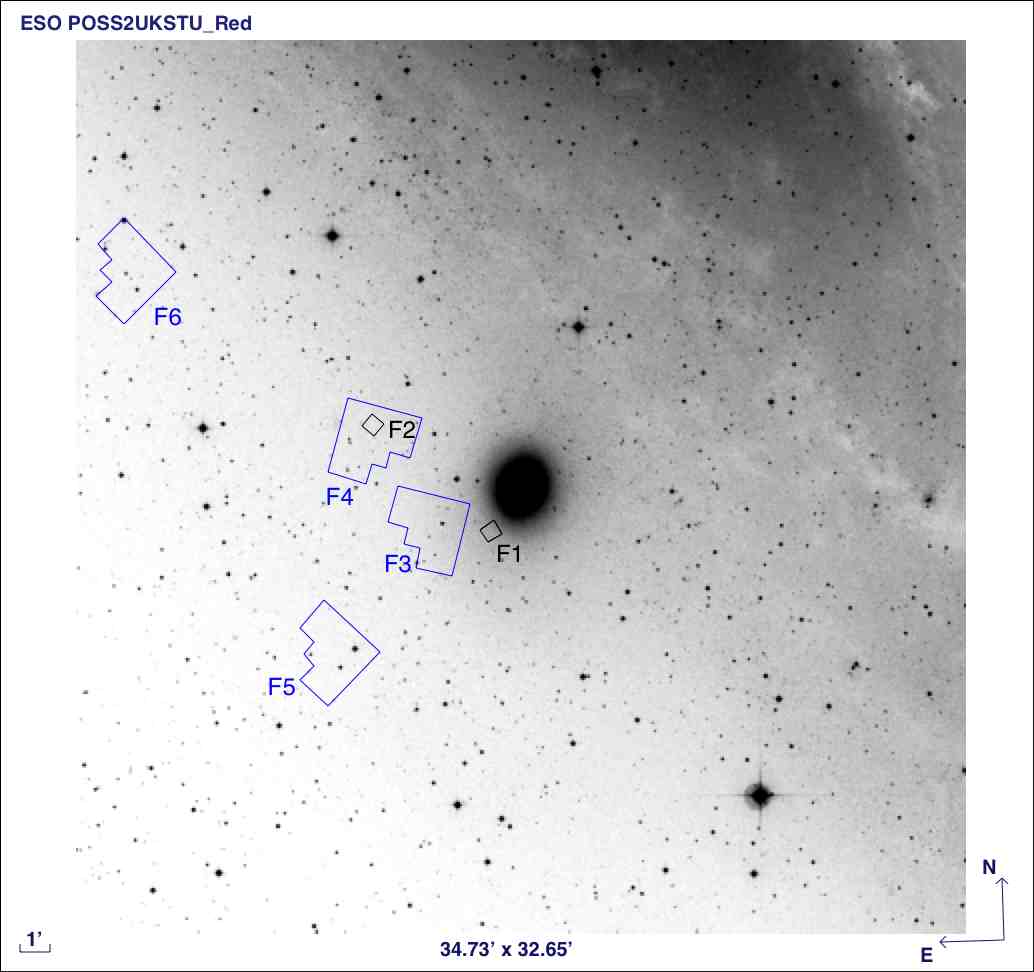
Figure 1.— Location of our two HST ACS/HRC pointings: M32 (F1) field and M31 background (F2) field, both indicated as black small boxes. Each field covers a region of $26\times 29\,\mathrm{arcsec^{2}}$ on the sky. The field F1 is located at 110″from the nucleus of M32 and represents the best compromise between minimizing image crowding and contamination from M31. The F2 field is at the same isophotal level in M31 corresponding to the location of the F1 field. Thirty-two exposures in each of the $F435W$ ($B$) and $F555W$ ($V$) filters were taken for each field. The location of fields F3, F4, F5 and F6 is also shown in blue. They are archival HST/WFPC2 fields near M32 that were analyzed in the Appendix to investigate the presence of a “blue plume”. Information about these observations can be found in Table  6. North is up and East is to the left.

2.2. Image Reduction, Stacking, and Upsampling

As outlined above, the data set for each of the four filter/field combinations comprises 32 exposures with non-redundant pointings. The images were combined in an iterative procedure designed to detect and repair cosmic-ray events, hot pixels, and other defects, with a Nyquist-sampled summed image as the final product.

The first reduction step was to interlace the four images at each position within the larger square-spiral dither pattern into a rough Nyquist image at that position. In practice, the sub-pixel dithers were accurate to $<0\farcs 01,$ so a simple interlace worked reasonably well for the initial reduction. For this first step, cosmic rays in one of the four images could be repaired by interpolation among the three remaining frames. The resulting eight Nyquist images were then shifted to a common centroid using sinc-interpolation (which does not smooth the data), and added to produce an initial stack. At this point the stack still contained artifacts from coincident cosmic-ray events within each of the eight subgroups, as well as hot pixels; although both types of artifacts are reduced in amplitude by the averaging implicit in the larger dither pattern.

The second reduction cycle used the initial Nyquist summed-image to then re-identify and repair cosmic-ray hits in each of the 32 raw images. Hot pixels were also identified and repaired at this stage by finding coincident events in detector, rather than celestial, coordinates. At this point a higher quality Nyquist summed-image was generated by combining all 32 images (trimmed to their common area) using the Fourier algorithm of Lauer (1999). This algorithm produces a summed image with double the native HRC pixel scale, by combining the images in the Fourier domain to eliminate aliased power from the under-sampled source images. The algorithm has no adjustable parameters, approximations, and so on, and important for the present application, induces no smoothing or degradation of the PSF.

The final reduction cycle was just to repeat the second cycle, but using the output from the second cycle as the input for the detection and repair of cosmic-ray events and hot pixels. The final summed image is thus essentially free of artifacts. As it eliminates the undersampling in the HRC, which provides the finest pixel scale of all HST instruments to begin with, it represents one of the highest-resolution images obtained with the observatory, given the blue-bands selected for the observations.

The final image still contains the geometric field distortion inherent to the HRC. Since the image is Nyquist-sampled, it can be rectified using sinc-interpolation, given the STScI two-dimensional polynomial representations of the distortion, without incurring degradation of the PSF. The required correction can be done by multiplying the image by the appropriate pixel area map (PAM). We construct a PAM image for the HRC which has a size of 2048$\times$2048 pixels, as this is the size of each combined image. The PAM is expressed in units of the pixel scale corresponding to our combined image, i.e., half of the native HRC scale, and it has an approximate value of $\sim$ 1.12 near the image center. We correct each combined image as follows:

$$\mathrm{CORRECTED_{flux}=COMBINED_{flux}\times PAM}$$ (1)

The combined images of F1 and F2 fields used for analysis thus have a pixel scale of $0\farcs 0125$ and a resolution of $\sim 0\farcs 05$ for point sources. They are shown in the top (F1) and bottom (F2) panels of Figure 2, in the $F555W$ filter, from which the strong crowding in these fields is clearly seen. There is however a difference between the stellar density in F1 and F2, as the crowding is more severe in F1 than in F2. The arrow in the top panel indicates the direction towards the center of M32.

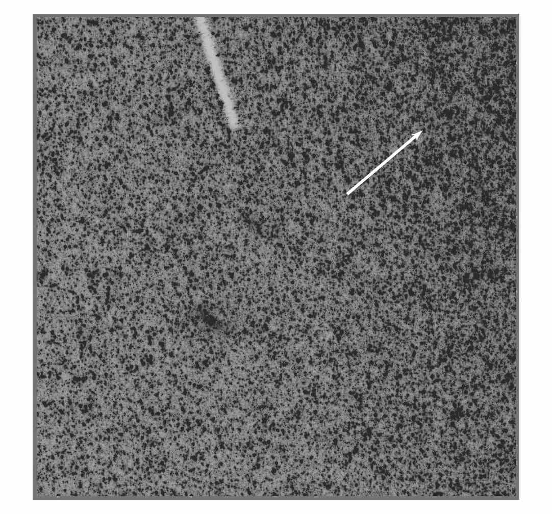
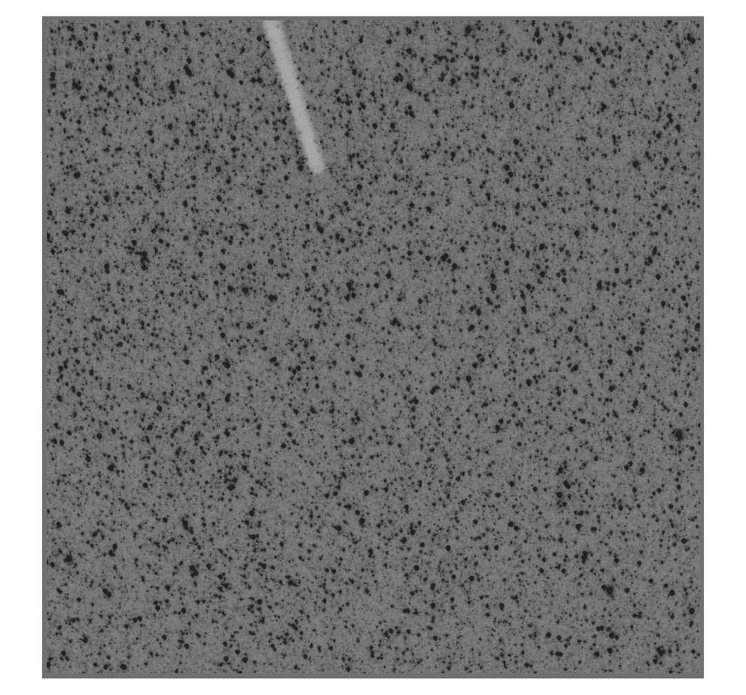
Figure 2.— Combined images of the 32 $F555W$ exposures in the F1 (top panel) and F2 (bottom panel) fields displayed with the same linear stretch. Each image has a size of 2048$\times$2048 pixels with a $0\farcs 0125$ pixel scale. There is a clear difference in stellar density between the images. This difference indicates that the crowding is more severe in F1 than in F2 field. We also note a stellar density gradient in the F1 image, becoming higher when approaching the center of M32, whose direction is indicated by the arrow in the top panel. The long white spot in the top center of each image is the occulting finger of the ACS/HRC coronagraph.

3. Photometry

The traditional method for extracting stellar photometry in crowded fields uses standard stellar photometry packages, e.g. DAOPHOT II (Stetson, 1987), which are specifically designed for this problem. This approach is favored over direct deconvolution of the PSF from the images, as HST images in general are undersampled, and deconvolution treats the artifacts due to aliasing as genuine sources (see Holtzman et al. 1991), resulting in large photometric errors. In the present case, however, the Nyquist-sampled and high-S/N summed images are free from artifacts. This motivated a re-examination of using general-purpose PSF deconvolution to mitigate the extreme crowding in the images, which we did in parallel to reducing the images with DAOPHOT II. To our delight, the deconvolved photometry is superior to that done with DAOPHOT, a conclusion based both on the sharpness of features in the CMDs derived from the images and extensive artificial star tests. We present derivation of stellar photometry using both methods in this section, showing why we decide in the end to solely use the deconvolved photometry for the analysis of the CMD.

3.1. DECONVOLVED IMAGE photometry

The final summed images of F1 and F2 were deconvolved using the Lucy-Richardson algorithm (Lucy, 1974; Richardson, 1972). The PSFs for the $F435W$ and $F555W$ images were constructed interactively and iteratively by summing the brightest relatively isolated stars in the images to produce ad hoc PSFs, which were then used to clean out the fainter stars in the wings of the PSF stars, resulting in improved PSFs, which were then used to refine the PSFs further. In all steps of the process, sinc-function interpolation was used to shift the PSFs and their component stars as needed.

The Lucy-Richardson algorithm works iteratively, quickly removing the “wings” of the PSFs, but taking considerably longer to enhance structure on the scale of the central diffraction cores. In the present case, we used 640 iterations on the $F555W$ images and 160 iterations on the $F435W$ images. This heavy level of deconvolution nearly transforms the images into a set of delta functions, but in doing so serves to split closely blended stars; pairs of stars as close as $\sim 0\farcs 03$ were separated. Due to its higher S/N, stars were identified in the $F555W$, while the $F435W$ image provided fluxes at the position of the identified stars. Stars were identified by a simple peak-finding algorithm. We had no formally-derived criterion for the threshold used to identify peaks. Instead, we examined faint sources in relatively isolated regions and adopted a single threshold for a given image that roughly separated what appeared to be real stars from noise fluctuations. In practice, the real depth of the photometry was established by the artificial star tests (ASTs) described after this section. We measured the stellar fluxes as follows. After the central pixel of the source was identified in the $F555W$ deconvolved image, we summed the counts within a $3\times 3$-pixel box centered at this position. The positions of the stars identified in the $F555W$ deconvolved image are used to find the stars in the $F435W$ deconvolved image. We measured the fluxes in the $F435W$ deconvolved in the same way, summing the counts within a $3\times 3$-pixel box around the central pixel of the source in the $F435W$ deconvolved image. All these steps were performed using algorithms running in the XVISTA package. The catalog of each field was cleaned of stars located in the borders, and in the occulting finger of the image. The final number of stars obtained with the deconvolution process is indicated in Table 2.

The deconvolved magnitudes needed to be corrected for a small non-linearity in the deconvolved flux. This is due to the fact that the fraction of flux in the box defined to measure the flux varies slightly with flux. We generated a correction table from simulated deconvolutions on a constant-sky level image. Stars were injected with appropriate Poisson noise as a function of flux. For each 0.2 step in magnitude we generated 16 stars per simulation and recover them performing the deconvolution in the same way as was done with the real stars. The correction is rather small (less than 0.1 mag) and only affects the magnitudes of some of the stars. Stars at both the brighter and fainter end are not affected by this small non-linearity.

In order to transform the instrumental magnitudes of the stars into apparent magnitudes, they need to be corrected for two effects that reduce the measured stellar flux: charge transfer efficiency (CTE) and aperture correction.

Charge Transfer Efficiency (CTE): Charge lost due to imperfect electron transfers from pixel to pixel and then to the readout amplifier degrades the photometry. Due to the gradual degradation of ACS after its installation in 2002, the effects of CTE are noticeable. The correction needed for ACS/HRC is given in the ACS Data Handbook:

$$\mathrm{\Delta mag=10^{A}\times SKY^{B}\times FLUX^{C}\times\frac{Y}{2000}}\times\\ \frac{(\mathrm{MJD}-52333)}{365}$$ (2)

where $\mathrm{A}=-0.44\pm 0.05$, $\mathrm{B}=-0.15\pm 0.02$ and $\mathrm{C}=-0.36\pm 0.01$ are the most recent coefficients (Chiaberge et al., 2009). In this formula, SKY is the sky level in electrons measured near the star, FLUX is the flux of the star in electrons, Y is the number of transfers which, when the default amplifier C has been used for readout as in our case, is simply the $\it{y}$ coordinate of the star. Finally, the images used to obtain the stellar magnitudes are constructed using images with very similar exposure times. Therefore, the SKY and FLUX values in the formula should be divided by the number of images used. The $\mathrm{\Delta mag}$ for each star is subtracted from its measured magnitude. Values of $\mathrm{\Delta mag}$ vary from 0.001 to 0.1.

Aperture Correction: The PSFs used for the deconvolution have limited extent stellar wings in order to avoid as much as possible the contamination by neighboring stars. Hence, the contribution of the flux in the large extent of the stellar wings need to be added to the measured magnitudes. The standard procedure to perform this correction consists of obtaining the flux for a small number of bright and isolated stars within a $0\farcs 5$ aperture radius, after all resolved stars – except those to be measured – have been removed. The median value of the differences between the magnitudes obtained from this flux and the one measured is the aperture correction (Stetson & Harris, 1988). This correction is then applied to all of the star magnitudes. After this step, the correction from $0\farcs 5$ to “infinite” is made using the tables in Sirianni et al. (2005). In our case, such bright and isolated stars are unavailable because the field is so crowded. Moreover, even if we could find some bright isolated stars, we would need to subtract an enormous number of stars from the image. The residuals from the PSF-fitting of all those subtracted stars will remain, adding fluctuations to the image and therefore significant errors to the photometric measurements. For these reasons we have decided to use the encircled energies (EE) which have been tabulated by Sirianni et al. (2005) and provide the fraction of the total source count as a function of the aperture radius, instead of the usual method. At each PSF radius, we calculate the fraction of flux that is missing and add this to the magnitudes. These values differ in each filter band and they are listed in Table 2 as well as the PSF radius used for the deconvolution, for each filter/field combination. We are aware that the aperture corrections calculated with the EE should only be applied to the photometric data for aperture radii larger than 10 pixels in the original HRC image, and therefore 20 pixels in our combined images. This was only the case for one of the PSFs we have obtained. However, due to the issues explained above, we have no other way to correct by aperture correction without introducing significant errors.

Finally, if $\lambda$ is the bandpass in the ACS/HRC system, the apparent magnitudes $\mathrm{m_{ap}}$ are transformed into the VEGAmag system using the zero points 36.73 and 36.80 for $F435W$ and $F555W$ respectively, which were obtained as follows:

$$\mathrm{ZP(\lambda)=2.5\log[t_{exp}(\lambda)]+ZP_{VEGAmag(\lambda)}}$$ (3)

The values for $\mathrm{ZP_{VEGAmag(\lambda)}}$ are 25.19 and 25.26 for $F435W$ and $F555W$ respectively.

Table 2Detections

	Detections	$R^{F435W}_{\rm{PSF}}$	$R^{F555W}_{\rm{PSF}}$	ACF435W	ACF555W
Deconvolution
F1	58,143	5	5	$-0.25$	$-0.22$
F2	27,963	6	16	$-0.22$	$-0.10$
DAOPHOT II
F1	50,583	6	6	$-0.22$	$-0.21$
F2	19,780	6	6	$-0.22$	$-0.21$

3.2. DAOPHOT photometry

We also performed stellar photometry with the standard DAOPHOT II and ALLSTAR packages (Stetson, 1987, 1994) to compare with the photometry obtained from deconvolved images.

We first built a PSF for each combined image from bright and as isolated as possible stars in each field of view (FoV). This was done iteratively using the PSF routine of DAOPHOT II. The number of stars that finally remain to construct the PSF is about 50 per image. After testing various PSF models, we adopted a “Penny” function (a sum of a Gaussian and a Lorentz function) as the best analytical model for all the images, according to the Chi value calculated by the PSF routine. We adopted a PSF that varies quadratically with position.

We performed PSF-fitting photometry on the images using ALLSTAR. The procedure was applied to a list of star candidates obtained from a DAOPHOT routine, from which concentric aperture photometry was performed to obtain crude apparent magnitude estimates and sky determination for all the objects found. Due to the severe crowding, the procedure of finding star-like objects, concentric aperture photometry and profile-fitting photometry was performed 3 times in order to both find the faint stars and improve the photometry on the bright stars. After this procedure we had four ALLSTAR output lists, one for each filter on each field, from which we retain only the objects having a statistically good photometry. We made use of the Chi value, sharpness index, and magnitude errors given by ALLSTAR to eliminate possible false photometric detections, e.g. background galaxies, unrecognized blends or cosmic rays. An extra step was performed and we cleaned each list of stars located both at the edge of the image, i.e. those stars having image coordinates X or Y either $<$ 23 or $>$ 2023, and in the occulting finger of the ACS/HRC CCD, for which the magnitudes were poorly determined.

We then used the DAOMATCH and DAOMASTER algorithms (Stetson 1994) to correlate the output list from the $F435W$ filter with the output list from the $F555W$ filter. This created a combined star catalog. An object was considered to be a star if it is found in both filters ($F435W$ and $F555W$) within a distance of 2 pixels. The final number of stars that we obtained for each field is listed in Table 2.

The last step consisted of applying the CTE and aperture corrections to obtain the apparent magnitudes in the VEGAmag system. This was done in exactly the same way explained in the above section. The PSF radius as well as the aperture correction values used for this photometry are indicated in Table 2 for each filter/field combination.

3.3. Comparison of the two photometric methods

To compare the two photometric lists, we first directly examine the CMD obtained from the deconvolved images with that obtained from the photometry performed using DAOPHOT. Figure 3 shows the deconvolved (left panel) and DAOPHOT (right panel) CMDs obtained for field F1. The same but for F2 is shown in Figure 4. We see that the deconvolved CMDs look better, as they produce notably clearer features at all luminosities. All of the features described in Section 5 are much sharper and better defined, and the outliers to the red of the RGB ($F435W-F555W>1.5$, $F555W=$ 25–27.5) are greatly reduced. In addition, a visual inspection of the subtracted images reveals that deconvolution does a considerably better job in resolving blended stars. Furthermore, we compared the results given by the ASTs (see Section 3.4 for a detailed description) using deconvolved images with that obtained using DAOPHOT. Figure 5 shows, in the top panel, the differences between the recovered and injected magnitudes obtained using deconvolved images (red dots) and DAOPHOT photometry (black dots), as a function of the injected magnitudes. The bottom panel shows the mean error of these differences as a function of injected magnitudes. For clarity, only the results of the same 10 ASTs (i.e. 20,000 injected stars analyzed) are shown. We can see that there is much more scatter in the DAOPHOT-recovered magnitudes at all magnitude levels; this is especially clear at the bright end. As shown in the bottom panel of Figure 5, the deconvolved photometry results in smaller errors than DAOPHOT. All this indicates that the photometry performed on the deconvolved images is superior to that obtained using DAOPHOT.

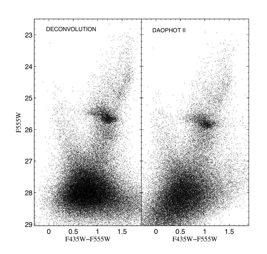
Figure 3.— ($F435W-F555W$, $F555W$) CMDs of field F1 obtained from the deconvolution (left-hand panel) and DAOPHOT (right-hand panel) photometry. They contain 58,143 and 50,583 stars respectively, and are calibrated onto the VEGAmag HST system. We can see that features in the deconvolved CMD are more clearly delineated than in the DAOPHOT CMD, at all luminosities. All of the features described in Section 5 are much sharper and better defined, e.g. the RGB and RC. Moreover, the outliers to the red of the RGB ($F435W-F555W>1.5$, $F555W=$ 25–27.5) are greatly reduced in the deconvolved CMD when compared with DAOPHOT. We therefore only use the deconvolved CMD for further analysis. See text for more details.

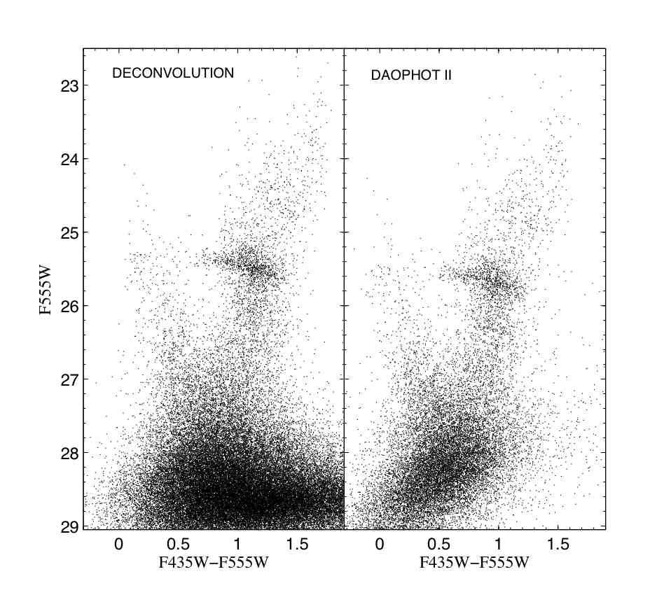
Figure 4.— Same as Figure 3 but for field F2.

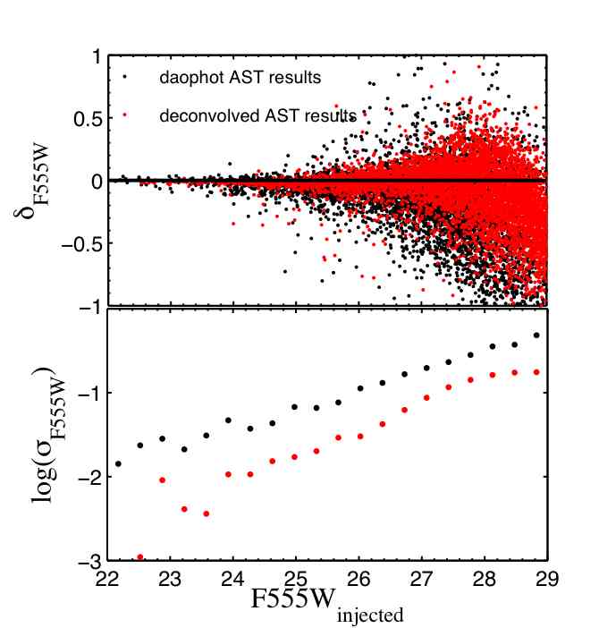
Figure 5.— Comparison of 10 ASTs results from deconvolved images (red dots) and DAOPHOT photometry (black dots). Top panel: (recovered $-$ injected) magnitudes as a function of injected magnitudes. Note the larger spread in the recovered DAOPHOT magnitudes compared with the deconvolved magnitudes, especially at the bright end. Bottom panel: Mean errors as a function of injected magnitudes. Errors are greatly reduced in the deconvolved photometry when compared with DAOPHOT.

Finally, we have also compared the list of stars obtained from both methods by cross-correlating them using DAOMATCH and DAOMASTER. The number of matched stars between deconvolved and DAOPHOT photometry was $\sim 32,000$ for field F1 and $\sim 17,000$ for field F2. Figure 6 shows the differences between the apparent magnitudes in both photometric results as a function of the deconvolved magnitudes. We find that there is an almost constant shift between the magnitudes of the matched stars, especially in the F555W filter, such that the deconvolved photometry produces systematically brighter magnitudes. To investigate the cause of this trend, we compare the PSFs used to deconvolve the images with the ones obtained using DAOPHOT and we found that the DAOPHOT PSFs have small wings or none at all. Due to the severe crowding in our fields, we could only generate reliable PSFs with very small radii, using DAOPHOT, which are essentially devoid of wings. We therefore believe that the PSFs constructed to deconvolve the images are more reliable and therefore so is the photometry based on the deconvolved images. Nevertheless, if we correct for the shifts in magnitudes, Figure 6 shows that both photometric methods agree well for $F555W<27$ and $F435W<27$. However at $F555W>27$ and $F435W>27$ the differences become significant. Looking at the locations of stars at these faint magnitudes, it appears that most of the sources are probably products of blends. Note that the detection limit in the deconvolved images is determined below to be at $F555W\sim 28$.

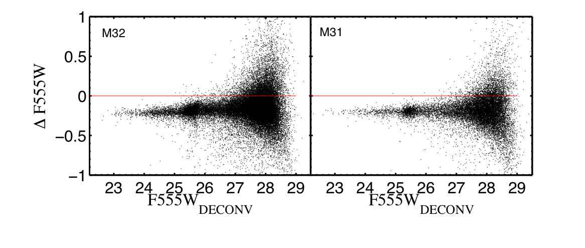
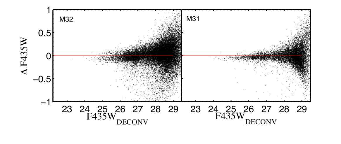
Figure 6.— Difference between stars found using deconvolved images and the ones found by DAOPHOT II as a function of the deconvolved apparent magnitudes. On the two top panels we show the differences in the $F555W$ filter (left-hand panel: F1, right-hand panel: F2) and on the two bottom panels we show the same but in the $F435W$ filter (left-hand panel: F1, right-hand panel: F2). Here $\mathrm{\Delta mag=mag_{DECONVOLVED}-mag_{DAOPHOT}}$. There is a constant shift between the deconvolved and DAOPHOT magnitudes that we attribute to a difference in the PSFs, considering deconvolution to be a more reliable method. Apart from the shift, there is however a reasonable good agreement between the two photometric methods for magnitudes $\lesssim 27.5$. The photometric results have little to do with each other for fainter magnitudes (see text for more details). Magnitudes are calibrated onto the VEGAmag photometric system.

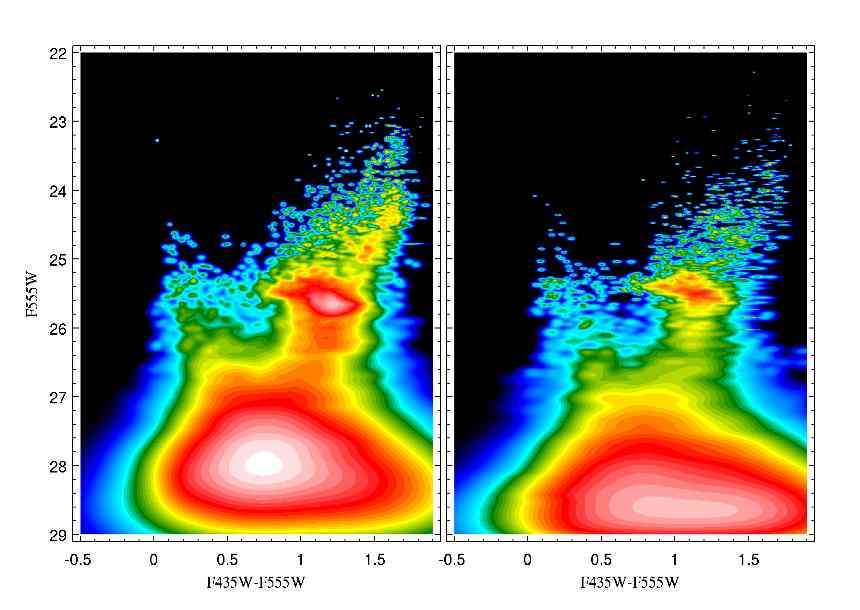
Figure 7.— ($F435W-F555W$, $F555W$) CMDs obtained from image deconvolution of F1 (left panel) and F2 (right panel) in an error-based Hess representation with a logarithmic stretch, where features are better highlighted. The error-based Hess diagram represents relative density of stars weighted by their photometric errors.

Due to all the above reasons, we are convinced that deconvolution, which has not been previously used to derive stellar photometry, gives remarkably better results than the standard photometric packages for these extremely crowded HST images. We therefore use the CMDs and the list of stars from the deconvolved images for further analysis. Figure 7 shows the F1 (left panel) and F2 (right panel) deconvolved error-based Hess diagrams with a logarithmic stretch, where the features are better highlighted. The error-based Hess diagrams represent relative density of stars weighted by their photometric errors as follows. Each star is represented by an elliptical gaussian with color and magnitude widths as a function of its color and magnitude photometric errors given by the ASTs (see next subsection). The color-magnitude image containing all these elliptical gaussians has been split into 600$\times$600 bins. Note that the two CMDs show a surprisingly similar morphology. We return to this point in Section 7.

3.4. Completeness tests and error analysis

When analyzing the data and before any detailed interpretation, it is necessary to have a good understanding of the completeness of the CMD as a function of both magnitude and color. The major source of incompleteness here is crowding, which is the most important limitation to the analysis of rich stellar fields. The well-known method of artificial stars (Stetson & Harris, 1988) is the best way to quantify its effects. Since the crowding effects are different for the F1 and the F2 fields, due to the differences in stellar density (Figure 2), such ASTs need to be carried out in each field separately to reach statistically significant results for both. The generation of artificial stars was done following the prescriptions introduced by Gallart et al. (1996) and using the IAC-STAR code (Aparicio & Gallart, 2004). This code generates synthetic CMDs by means of interpolation in the metallicity and age grid of a library of stellar evolutionary tracks. This interpolation results in a smooth distribution of stars following a given star formation rate, initial mass function and chemical enrichment law. In order to apply the AST method it is important that the magnitudes and colors assigned to the artificial stars are realistic, covering a range as wide as the populated one by the real stars to fully sample the observed colors and magnitudes. It is important that the injected stars have realistic colors to test for color effects. We generated a synthetic CMD of 500,000 artificial stars adopting a constant star formation rate with ages from 0 to 14 Gyr, and metallicities $0.0001<Z<0.04$ uniformly distributed at all ages. We have chosen a limiting magnitude for the synthetic stars of about two magnitudes fainter than the fainter stars observed in our CMD, to explore the possibility of recovering a very faint, unresolvable artificial star as if it were much brighter. The synthetic CMDs given by IAC-STAR are expressed in a photometric magnitude system different than the ACS/HRC photometric system. In particular we have chosen the bolometric correction library from Origlia & Leitherer (2000), which has magnitudes in the HST WFPC2 system. We therefore have transformed those magnitudes into the ACS/HRC photometric system using the transformation given by Sirianni et al. (2005). Since the artificial stars need to be injected into the images, the synthetic CMD needs to be transformed to instrumental magnitudes. Hence we have converted the absolute magnitudes given by the synthetic CMDs into apparent magnitudes using a distance modulus of $\mu_{0}=24.43$ (Ajhar et al., 1996), a reddening of $E(B-V)=0.08$ (Burstein & Heiles, 1982), and an extinction of $A_{F555W}=0.25$ (Sirianni et al., 2005). We have then applied the photometric corrections in reverse order to obtain the artificial stars onto the raw magnitude system. The artificial stars are placed into the images with random pixel locations using the PHOTONS routine in XVISTA. The number of artificial stars injected per experiment should not be larger than about 5% of the real stars found in the images (see e.g. Grillmair et al., 1996a; Fuentes-Carrera et al., 2008) to avoid a significant increase of the (already extreme) crowding in the images. We have used 2,000 artificial stars per AST. Once the artificial stars are placed into the images, photometry was performed using deconvolved images as before, since it is the deconvolved photometry that we use for the CMD analysis. The reduction of the original and artificial images must be carried out identically for the comparison to be valid. A second requirement for a valid AST is that the reductions should be performed without knowing which stars in the synthetic frame are added and which are real. For each AST we obtain a deconvolved photometry list as output file. Then, we append the file containing the injected positions and magnitudes of the artificial stars to the output file from the original photometry of real stars. Next we match this appended file with the star list of the artificial image. This provides us with a list of recovered stars, i.e., injected stars that are paired with stars from the artificial stars subset. The matching is done with DAOMATCH and DAOMASTER using the two star lists as two lists to be matched. Stars within 1 pixel of radius distance are considered to be recovered. This process has been repeated as many times as necessary in each image in order to achieve a very large number of artificial stars analyzed and to recover a number of stars similar to the one of real stars in the image. In this way, we can statistically sample the whole CMD diagram, both in magnitude and color indices. In total $\sim 5\times 10^{5}$ stars have been used to perform $\sim$ 250 ASTs on each image. The procedure is applied to both filters of each field, i.e. F1 and F2.

A comparison between the number of injected and recovered artificial stars provides information about the crowding effects on the photometry and gives us the completeness level of our data. We define the completeness factor as the fraction of recovered stars in a given color-magnitude bin as follows:

$$\Delta_{i,j}=\frac{N^{rc}_{i,j}}{N^{in}_{i,j}}$$ (4)

where $N^{rc}_{i,j}$ is the number of stars whose recovered color indexes and magnitudes lie in the $i,j$ color magnitude bin, and $N^{in}_{i,j}$ is the number of stars whose injected color indexes and magnitudes lie in the $i,j$ color magnitude bin (Gallart et al., 1996). The data were divided for this calculation into 20 bins in both magnitude and color. Figure 8 shows the completeness fractions obtained for both the F1 and F2 fields. The color bar in these figures indicates the values of the completeness fraction level, increasing from 0 to 1, where 1 represents 100% completeness. The magnitudes in these figures are expressed in the VEGAmag system. The 50% completeness level for F1 is located at $F555W\sim$ 28 ($F435W\sim$ 28.5) independent of color. Our completeness factor falls rapidly to zero below $F555W\sim 28$, suggesting a limiting magnitude $F555W_{lim}\sim 28$. The 50% completeness level for F2 is half a magnitude deeper, at $F555W\sim$ 28.5, indicating again that this field is slightly less crowded.

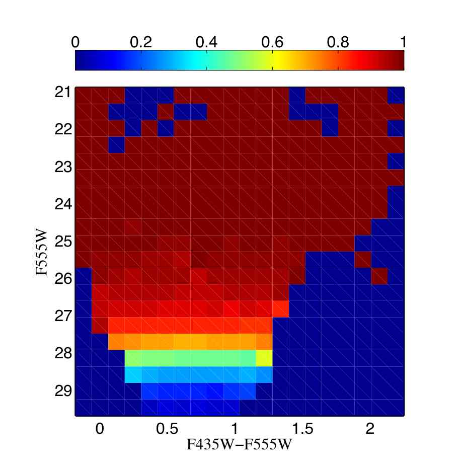
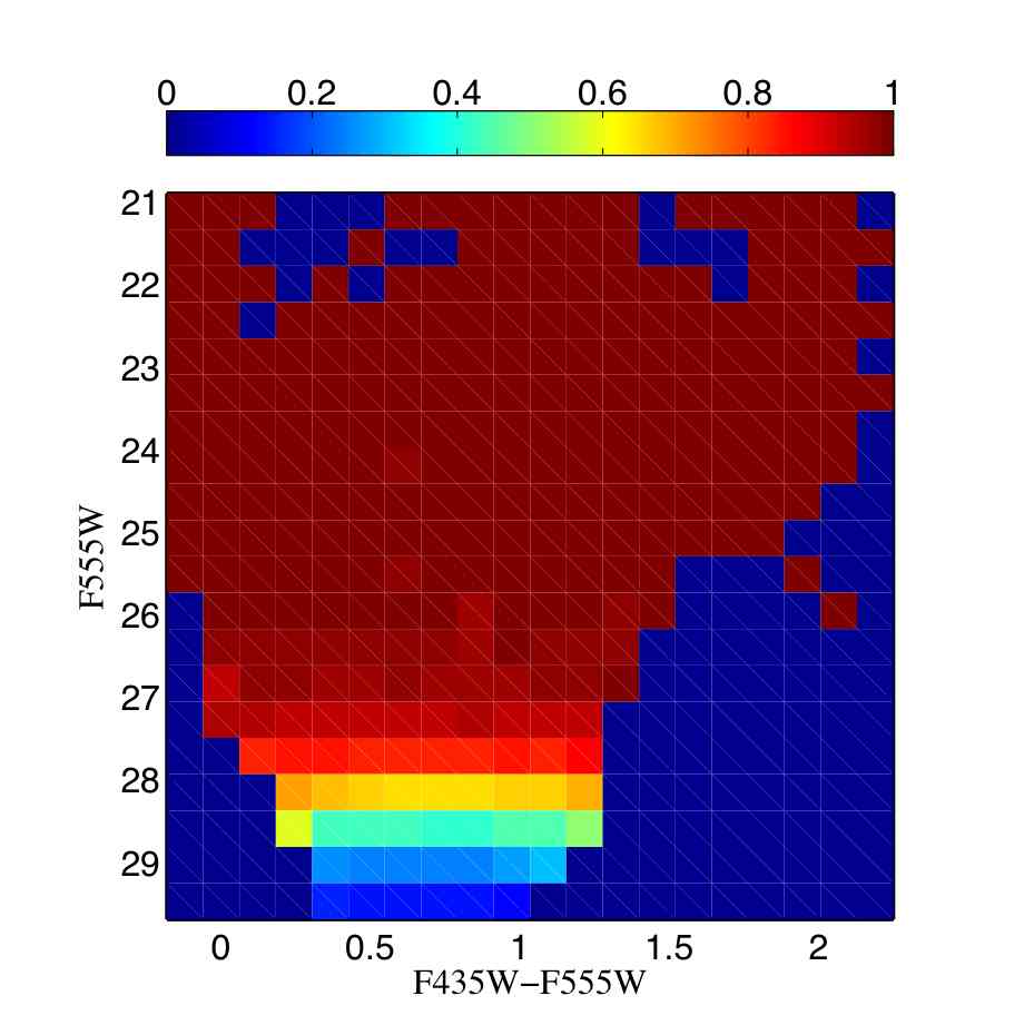
Figure 8.— Completeness fractions for fields F1 (left-hand panel) and F2 (right-hand panel) as a function of apparent $F555W$ magnitudes and $(F435W-F555W)$ colors. The values of the completeness fraction are determined for a given bin $i$,$j$ of magnitude $i$ and color $j$, indicated by the color bar. For field F1 the 50% completeness level is at $F555W\sim 28$. In the F2 field the 50% completeness level is at $F555W\sim 28.5$, half a magnitude deeper, indicating a less-crowded field than F1.

The actual photometric errors are quantified as the difference in magnitude between the recovered and injected stars, shown in Figure 9 for F1. In this figure the difference $\mathrm{\delta mag=mag_{recovered}-mag_{injected}}$ is plotted as a function of the injected magnitudes in both $F555W$ (left-hand panels) and $F435W$ (right-hand panels) filters. The completeness fractions as a function of magnitude are plotted in the bottom panels of the same figure. The median of the magnitude differences is negligible for magnitudes having more than 70% completeness. We see from these figures that the magnitudes of some recovered stars differ significantly from their input magnitudes, having significantly negative $\mathrm{\delta mag}<-1$ (i.e. recovered brighter). The appearance of aberrant stars coincides with the dramatic drop in the completeness at $F555W\sim 28$. These might be stars that were only detected because they are located at noise spikes. We therefore do not consider stars with magnitudes that lie below our 50% completeness level as recovered.

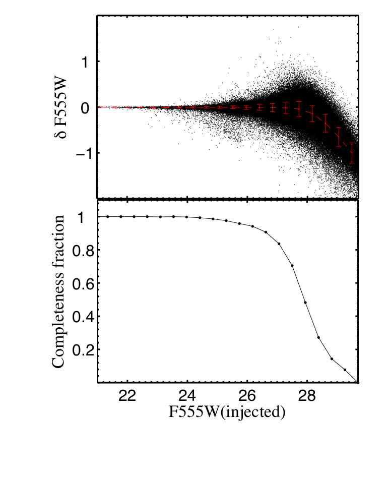
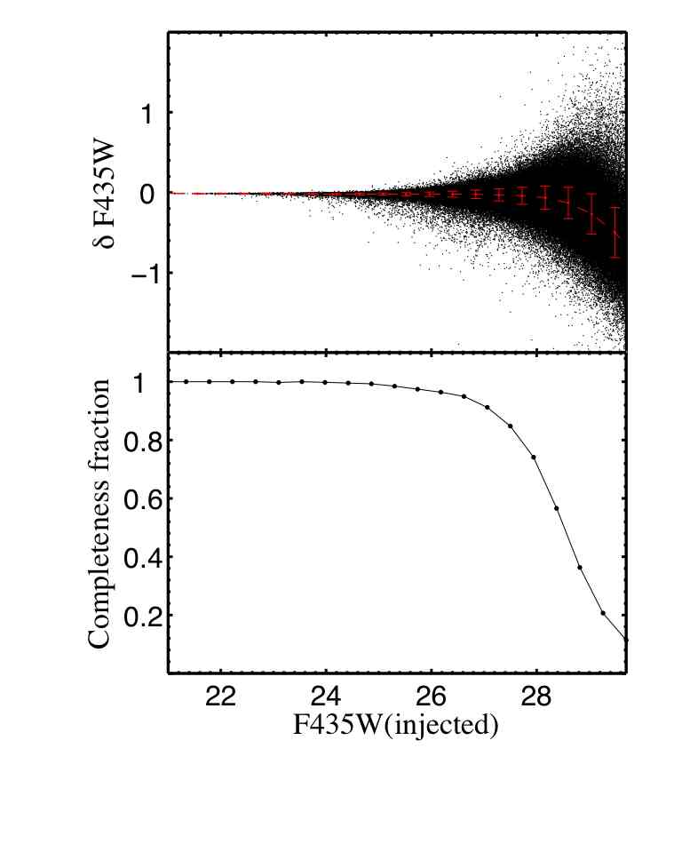
Figure 9.— Results from ASTs for field F1. (Recovered $-$ Injected) $F555W$ (left-hand panel) and $F435W$ (right-hand panel) as a function of the injected magnitudes are shown in the top panels. The 1-d completeness fraction as a function of magnitude is given in the bottom panels and it follows the theoretical color-magnitude locus of the M32 stars. The mean photometric errors as a function of magnitude are indicated. The median of these differences and the error of such medians are illustrated as red curves and red error bars respectively. Stars whose recovered magnitudes differ significantly ($|\delta\rm{mag}|\geq 1$) from their input magnitudes are products of blends and we do not consider them as recovered.

Photometric errors are defined for a given bin of magnitude $i$ and color $j$ as the errors in the median of the magnitude differences in that bin. We show in Figure 10 the amplitude of photometric errors throughout the theoretical CMD locus of the M32 stars. Our photometry shows excellent accuracy for magnitudes $F555W<26.5$ and the mean errors in magnitude and color are $\sim 0.18$ mag and $\sim 0.23$ mag, respectively at the 50% completeness level.

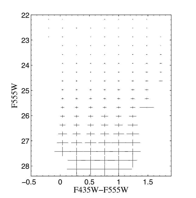
Figure 10.— Photometric color and magnitude errors for the CMD of M32, estimated from the ASTs. The errors are negligible ($<0.05$ mag) for stars brighter than $F555W=26$ and start to become significant ($>0.1$ mag) for stars fainter than $F555W\sim 27$.

We want to emphasize that a same AST analysis was additionally reproduced using DAOPHOT. As shown in Figure 5, we have obtained larger photometric errors with DAOPHOT photometry and much more scatter in recovered magnitudes. Thus, the ASTs were also used to prove quantitatively that the deconvolved photometry is superior than DAOPHOT.

4. M32 field decontamination

4.1. M31 contamination

M31 is clearly the dominant source of contamination in our M32 field (F1). M32 lies at a projected distance of 5.3 kpc south of the center of M31 and therefore contamination from its disk and bulge is significant. Moreover, at the position in which the F1 field was taken, the closest possible to the center of M32 without being overwhelmed by crowding effects, one third of the light is coming from M31. To correct for this statistically, we have also obtained images of a comparison field located at the same isophotal level within M31. As explained in previous sections, those images were processed in the same way as the F1 images.

Since both fields are located at the same isophotal level in M31, correcting for M31 stars would require that for each F2 star we subtract the closest one in color and magnitude from the F1 star list. However, as we have already addressed in previous section, the crowding differs between the two fields. Image crowding is more important for F1 than for F2 so there are different levels of completeness in the images that should be taken into account. We therefore cannot simply subtract the F2 stars from the F1 CMD in a “one-by-one” way. Instead, the number of stars removed from F1 depends on the completeness fractions computed at F1 and F2 fields (e.g., Gallart et al., 1996). Assuming that the population of M31 stars is statistically the same in both the F1 and F2 fields, we corrected the F1 CMD as follows: For each F2 star of magnitude $i$ and color $j$ an ellipse was defined in the F1 CMD centered at $i$, $j$ and with semi axes $err_{i}$ and $err_{j}$. The semi-axes correspond to the magnitude and color photometric errors, estimated from the ASTs, affecting the given region of the F1 CMD. We also consider the photometric errors in magnitude and color affecting the corresponding region of the F2 CMD when generating the semi-axes of the ellipse. For a given ellipse in the contaminated F1 CMD, a number $F_{n}$ of stars was subtracted randomly from the F1 list, where

$$F_{n}=\frac{\Lambda_{i,j}^{\mathrm{F1}}}{\Lambda_{i,j}^{\mathrm{F2}}},$$ (5)

and $\Lambda_{i,j}^{\mathrm{F1}}$ and $\Lambda_{i,j}^{\mathrm{F2}}$ are the corresponding completeness factors for F1 and F2 in the $i$,$j$ bin of the CMD (Gallart et al., 1996), as previously calculated. The closest integer to $F_{n}$ is chosen as the number of stars to be subtracted. If the number of stars in a given ellipse is smaller than the number of stars expected to be removed, we enlarge the semi-axes of the ellipse by a factor of two. The remaining stars are deleted from this larger ellipse in order of proximity to the color and magnitude of the F2 field star considered. This happens most often in regions of the CMD where the density of stars is low. The advantage of this process (Gallart et al., 1996) is that the region in magnitude and color from where the stars are removed varies along the CMD, i.e. the interval in magnitude and colors from which stars are removed is changing size depending on the photometric errors. Thus, brighter stars – the ones with smaller photometric errors – are subtracted from a small region around the field star in the CMD, whereas the fainter stars, and therefore the ones with larger photometric errors, are allowed to be removed from a larger region of the F1 CMD with a size controlled by the error.

We show in Figure 11 the F1 CMD decontaminated from the M31 background stars. The 50% completeness level is also shown in this Figure.

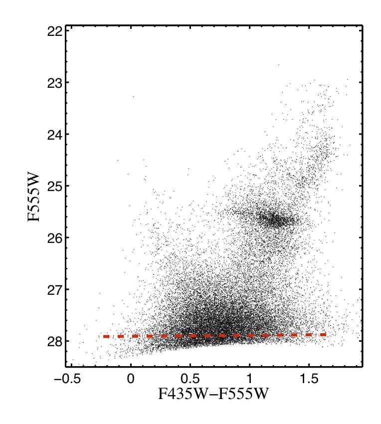
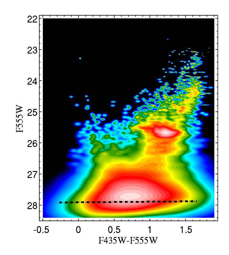
Figure 11.— Left panel: CMD of M32, corrected for contamination by the M31 background stars. The different crowding levels between the F1 images and the F2 images were taken into account to statistically perform the decontamination (see text for more description). Right panel: Error-based Hess representation of the decontaminated CMD of M32, where the features are better highlighted. To construct this Hess diagram, the stars were replaced by elliptical gaussians with color and magnitude photometric errors as color and magnitude gaussian widths, respectively. The CMD was then divided into 600$\times$600 bins. In both panels, the dashed line indicates the 50% completeness level of our data. Apparent magnitudes are calibrated onto the VEGAmag ACS/HRC system.

The number of M32 stars remaining after this decontamination process is $\sim 26000$ of the 58143 originally detected in F1 (Table 2).

4.2. Galactic foreground stars

Our field F1 is quite small, and the contamination by the Galactic foreground stars is very small. We have however still estimated it from star count data. The Besançon group model of stellar population synthesis of the Galaxy (Robin et al., 2003) predicts the amount of stars in a given magnitude interval for a given location. This model predicts 14 foreground Galactic stars in the range of $V=22-30$ in our $\sim 29\,\mathrm{arcsec^{2}}$ ACS/HRC field. This is of course negligible compared with the thousands of stars we have obtained in our photometric catalog, and therefore we do not consider foreground stars further in our analysis.

5. The Stellar Populations of M32

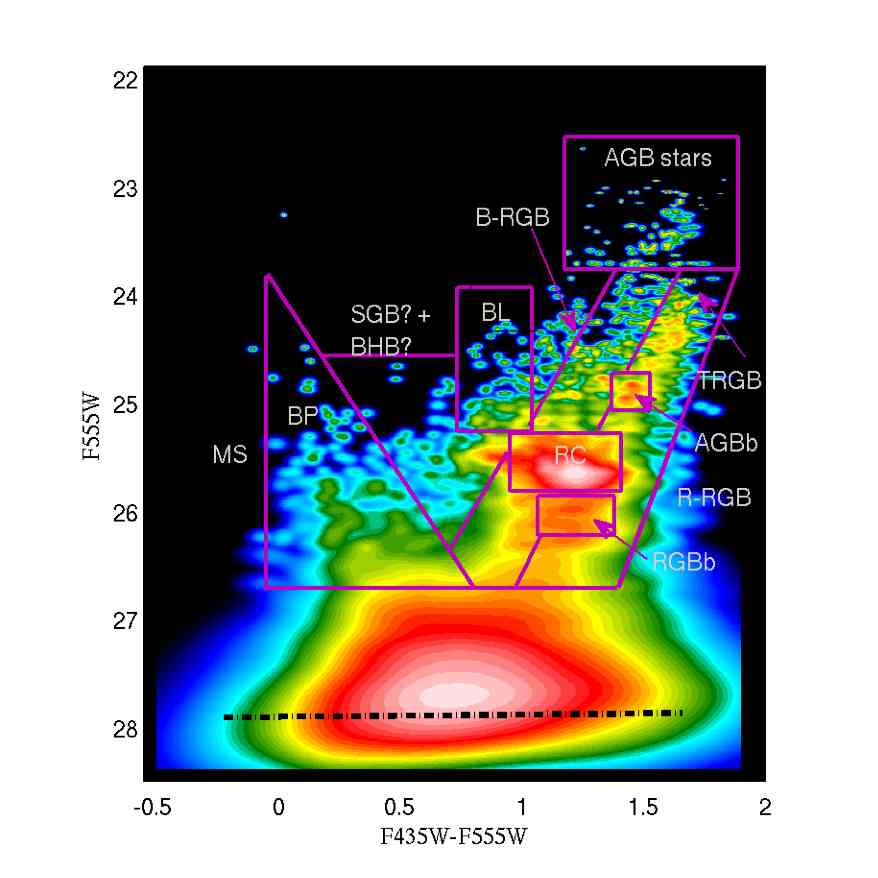
Figure 12.— Error-based Hess diagram for M32, corrected for contamination by the M31 background stars. The boxes indicate various features that represent different stellar populations. MS: Main Sequence; BP: Blue Plume; SGB: Subgiant branch; BHB: Blue Horizontal Branch; BL: Blue Loop; RC: Red Clump; RGBb: Red Giant Branch bump; R-RGB: Red-Red Giant Branch; B-RGB: Blue-Red Giant Branch; TRGB: Tip of the Red Giant Branch; AGB: Asymptotic Giant Branch; and AGBb: Asymptotic Giant Branch bump. The dotted-dashed line indicates the 50% completeness level of our data. Magnitudes are calibrated onto the VEGAmag system.

The CMD we have obtained is deep enough to allow a comprehensive study of the stellar populations of M32, and we can gain some insights into them by comparing our CMD with theoretical isochrones. In what follows we present the most detailed resolved photometric study of M32 carried out so far. Figure 12 shows the CMD of M32 with boxes highlighting features that reveal the different stellar populations. We see evidence for an intermediate-age and old population – ages between 2 and 10 Gyr – due to the presence of a strong red clump, an extended and bright asymptotic giant branch, a prominent red giant branch, and the red giant branch bump as well as the asymptotic giant branch bump. We also see possibly evidence of a young population – ages younger than 2 Gyr – due to the presence of stars occupying the blue plume producing an extended main sequence, blue loop stars, and a possible bright subgiant branch. Evidence of an ancient – older than 10 Gyr – population could be represented by blue horizontal branch stars together with a well-populated red giant branch. Note that a well-defined blue horizontal branch in our CMD is not present, but we have observed RR Lyrae stars in F1 (F10) and there are stars in the region where we would expect to see blue horizontal branch stars. We emphasize here that all these features are above the 80% completeness level where the photometric errors are very small. Hence what we see in the CMD at this level represents the intrinsic properties of the stars. Note in Figure 12 that, although we have the highest resolution and deepest data for M32 yet obtained, the severe crowding of our fields makes it impossible to reach the oldest main-sequence turn-offs. This unfortunately will remain a challenge beyond existing telescopes and even near-future space-telescopes such as JWST.

In the following, we discuss the different stellar populations of M32 in detail. We assume a distance modulus (DM) of $\mu_{0}=24.53$ (this paper, below), Galactic reddening $E(B-V)=0.08$ (Burstein & Heiles, 1982), and extinction $A_{F555W}=0.25$ (Sirianni et al., 2005). Note that we have only considered Galactic reddening, on the assumption that M32 is dust-free. We note that no dust features are seen in the surface photometry residual maps of the M32 center (Lauer et al., 1998) or envelope (Choi et al., 2002). F10 tested for internal extinction in F1 and F2 due to M31 and/or M32 by using the intrinsic properties of the RR Lyrae variables in the fields. They found that the mean reddening values obtained in both fields agree within the errors and are further consistent with the assumed Galactic reddening. We also tested for differential extinction over the HRC field by comparing the RGB colors of CMDs constructed at different quadrants of the image and found no difference. We use theoretical isochrones from the Padova library (Marigo et al., 2008; Girardi et al., 2002, 2008) as they are available in the HST ACS/HRC photometric system at different ages and metallicities. The metallicity in these models assumes $\mathrm{[M/H]=\log}(Z/Z_{\odot})$, $Z_{\odot}=0.019$, and $[\alpha/\mathrm{Fe}]=0$. Although our photometry could be transformed onto traditional magnitude systems (e.g., Johnson–Cousins) for comparison to other theoretical isochrones, such transformations always introduce significant systematic errors (Sirianni et al., 2005) and we prefer to stay as much as possible in the original photometric system of the data.

5.1. Intermediate-age (2 $\leq$ Age $\leq$ 8 Gyr) and old (8 $<$ Age $\leq$ 10 Gyr) populations

5.1.1 The Red Clump (RC)

The most prominent feature in our CMD is the RC formed mostly by the reddest low-mass stars burning helium in their cores. A strong RC, as we see here, indicates the presence of intermediate-age/old metal-rich stars. Models of core-helium burning stars predict that the RC luminosity depends on both age and metallicity (Cole, 1998; Girardi et al., 1998). For a given metallicity, old stars form a fainter RC than young stars whereas for a given age, lower metallicity stars form a brighter RC. For a population of known age and metallicity, the RC is at a fairly constant color and luminosity, hence these stars can serve as good standard candles to derive distances both within our own Galaxy and to nearby galaxies and globular clusters (Percival & Salaris, 2003). We make use of this fact to derive the distance to M32 in Section 6.

We now attempt to estimate a mean age and metallicity of M32, based on the constraints that the presence of this feature impose. Constraints on age and metallicity of these populations can be obtained from the analysis of the locus and width of the red giant branch (RGB) together with the position of the RC (Ferguson & Johnson, 2001; Rejkuba et al., 2005).

Table 3M32 RC, RGB$\mathrm{b}$ and AGB$\mathrm{b}$ magnitudes and colors.

	$F555W$	$(F435W-F555W)$	V	$\Delta V\rm{(bump-RC)}$
RC	$25.66\pm 0.08$	$1.20\pm 0.08$	$25.33\pm 0.09$	$\cdots$
RGBb	$26.21\pm 0.10$	$1.15\pm 0.18$	$25.89\pm 0.10$	$0.56\pm 0.13$
AGBb	$24.87\pm 0.09$	$1.44\pm 0.03$	$24.52\pm 0.09$	$-0.81\pm 0.13$

Note. — Errors are $1\sigma$ deviations.

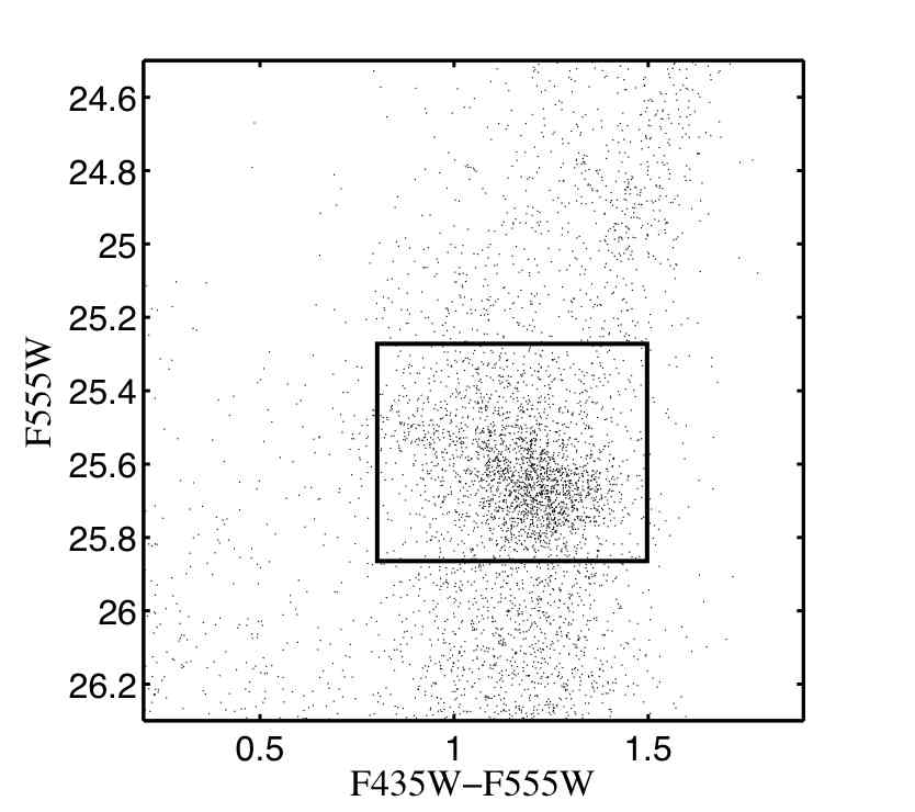
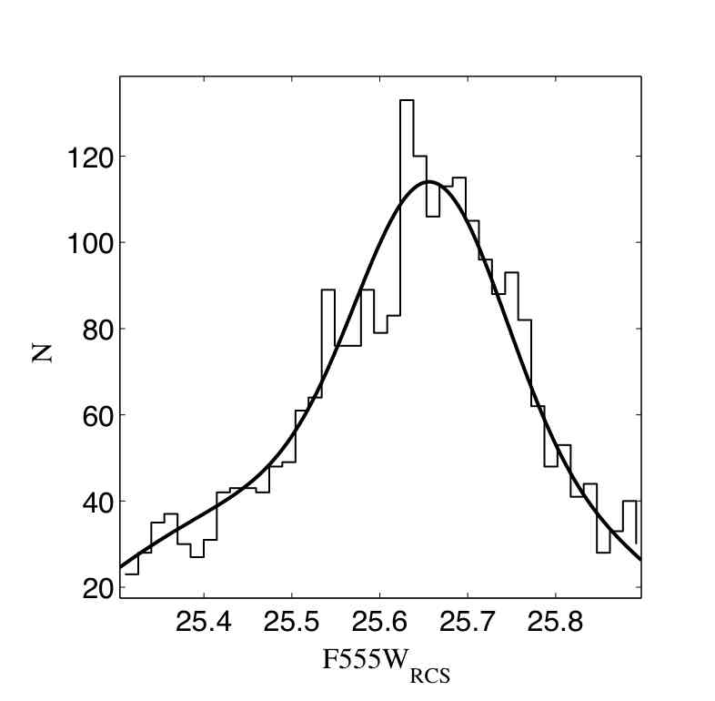
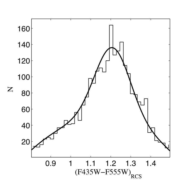
Figure 13.— Top panel: Close-up of the M32 CMD corrected for M31 background contamination in the region of the RC. Note the complex morphology of the RC. We observe a bluer and brighter end of the RC, at $F435W-F555W\sim 0.75$, which indicates the presence of lower metallicity stars in combination with young stars at the bottom of the blue loop. The red end of the RC, at $F435W-F555W\sim 1.30$, is fainter, which indicates the presence of both older ages and higher metallicities stars. Stars inside the box $25.30\leq F555W\leq 25.90$ and $0.80\leq(F435W-F555W)\leq 1.50$ are selected to determine the mean apparent magnitude of the RC in our field. In total 2525 stars lie inside this box. Bottom panel: A non-linear least-squares fit of the function $N(F555W)$, Equation 6 (Paczynski & Stanek, 1998), to the histogram of stars in the clump region is shown in the left-hand panel. $N(F555W)$ is a Gaussian representing the RC population plus a second term representing the RG stars that contaminate the RC selection. The coefficients found for this fit with 95% confidence bounds are $F555W_{m}$ = 25.66 and $\sigma=0.082$. In the right-hand panel we show the fit to the histogram of the color distribution of RC stars. The same formalism was used in this case and we obtain $(F435W-F555W)_{m}=1.20$ and $\sigma=0.088$.

We begin by measuring the mean luminosity and color of the RC. We consider a rectangle in the CM plane with $25.30<F555W<25.90$ and $0.80<(F435W-F555W)<1.50$ defined in such a way that all the RC stars remain inside it (Figure 13). We find 2525 stars in this rectangle; note that some of these will be RGB stars. Note in Figure 13 the complex morphology of the RC in the CMD of M32. As stated above, the RC’s morphology depends not only on the metallicity but also on the age of the stellar system. In this case we observe a bluer and brighter end of the RC, at $F435W-F555W\sim 0.75$, which indicates the presence of lower metallicity stars and young intermediate-mass stars at the bottom of the blue loop (see next subsection). The red end of the RC, at $F435W-F555W\sim 1.30$, is fainter, indicating the presence of both older ages and higher metallicities stars. We will quantitatively study the complex morphology of the RC when deriving the SFH of M32 in a follow-up paper. We make a histogram of the luminosity of these stars and measure the peak magnitude of the RC by fitting the $F555W$-band luminosity function with the following function from Paczynski & Stanek (1998),

$$N(F555W)=a+b(F555W-F555W_{m})+\\ c(F555W-F555W_{m})^{2}+\frac{N_{RC}}{d}e^{-\left[\frac{(F555W-F555W_{m})^{2}}{2\sigma^{2}_{RC}}\right]},$$ (6)

a Gaussian representing the RC population plus terms representing the contamination due to RGB stars. Here, $F555W_{m}$ is the mean apparent magnitude, $\sigma_{RC}$ is the width of the RC and $N_{RC}$ is the number of stars selected to determine the apparent magnitude of the RC. A non-linear least-squares fit of this function to the histogram of stars in the clump region provides $F555W_{m}$ and $\sigma_{RC}$. We show in the top panel of Figure 13 the stars inside the box that were selected to determine the mean apparent magnitude of the RC in our field. In the lower left-hand panel of the same figure we show the histogram of the magnitudes of those RC stars together with the fit. We can see that the data are well fit by this function. The mean color of the RC is calculated using the same formalism (lower right-hand panel of Figure 13) and its value, as well as the mean magnitude of the RC, is listed in Table 3. Models by Marigo et al. (2008) and Girardi et al. (2008) suggest, for the observed mean magnitude and color of the RC, a mean age of M32 of 8–10 Gyr for a metallicity $Z=0.012$ ([Fe/H]$\sim-0.2$ dex, see Section 5.1.3) consistent with the bulk of the stellar population being old.

There are uncertainties in this estimate: The mean magnitude and color of the RC are also well fit with a mean stellar population of 5 Gyr and solar metallicity $Z=0.019$, reflecting the age-metallicity degeneracy that occurs in the RGB. Moreover, the uncertainties in the distance modulus obtained (see below) could modify these parameters, possibly changing the mean age by $\pm 2$ Gyr.

5.1.2 The RGB bump (RGBb) and the AGB bump (AGBb)

We detect for the first time in M32 a feature in the RGB that we identify as the RGB bump (RGBb) located at $F555W\sim$ 26.10 (see Figure 12). This feature is the consequence of the following process that occurs at the beginning of the RGB phase. During evolution along the RGB, the H-burning shell moves away from the core of the star, which is increasing in luminosity at almost constant temperature. As the shell moves out to regions of ’fresh’ hydrogen it encounters the chemical discontinuity left behind by the maximum penetration of the convective envelope. When this happens, the rate at which the star climbs the RGB drops for a short period and even reverses for a while, until the shell adapts to the new environment, and then the star again increases its luminosity, burning in a regime of constant H content. As a result, the star crosses the same small portion of the RGB evolutionary path —the same luminosity interval— three times, producing a peak in the luminosity function (Iben, 1968; Sweigart & Gross, 1978; King et al., 1985; Renzini & Fusi Pecci, 1988). The time that a low mass star spends during the RGBb phase is a considerable fraction ($\sim$ 20%) of the total RGB lifetime, and the RGBb can be easily observed in an intermediate-age or old stellar system provided there is a large number of stars. Stellar evolution models predict that the brightness of this feature depends on both the age and metallicity of the system. For a given metallicity old stars have a lower RGBb luminosity than young stars (Alves & Sarajedini, 1999, hereafter AS99).

We calculate the mean magnitude of the RGBb by fitting a Gaussian plus a quadratic function to the $F555W$-band luminosity function around the bump (Figure 14). The bin size of the distribution is 0.1 mag, since this is the approximate mean photometric error in this region of the CMD. The mean color of the RGBb was obtained by fitting a Gaussian to the color distribution around the bump; the inferred value and its standard deviation are listed in Table 3. We can estimate the significance of this bump by comparing the number of RGB background stars (i.e. the quadratic component of the fit) with the number of stars that are in the bump (the Gaussian component of the fit). There are $1127\pm 34$ RGB background stars, where the error is simply Poisson error. The number of remaining stars that are in the RGB bump is $219\pm 51$. Thus, the RGB bump is a $5$–$8\sigma$ detection.

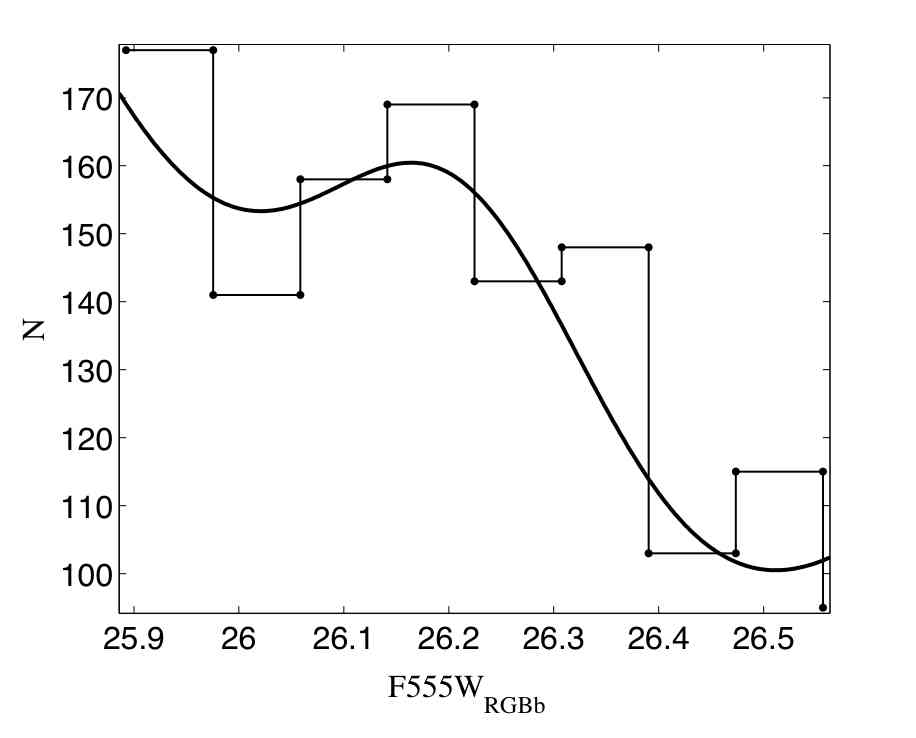
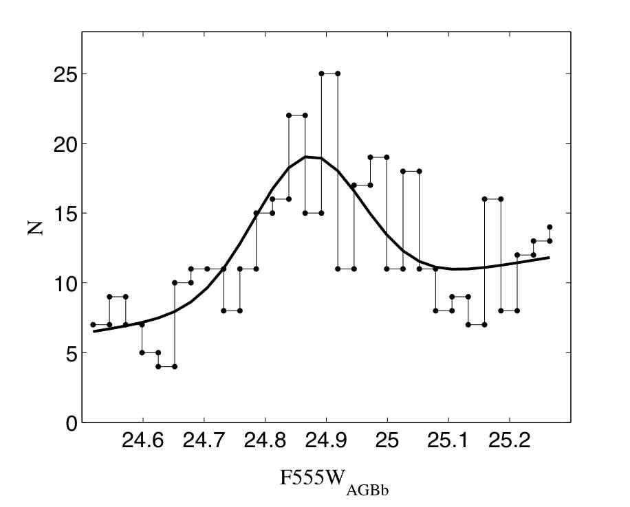
Figure 14.— Left-hand panel: A Gaussian plus a quadratic fit to the $F555W$-band luminosity around the RGB bump. A number of 1370 stars lie in this region. The peak is at $F555W$ = 26.21 and $\sigma=0.10$. The bin size of the luminosity function is 0.1 mag, since this is the approximate mean value of the photometric errors in that region of the CMD. From this fit, we find that the RGB bump is a $5$–$8\sigma$ detection. Right-hand panel: A Gaussian plus a straight line fit to the histogram of stars in the AGB bump region. The peak is at $F555W$ = 24.87 and $\sigma=0.09$. A number of 372 stars lie in the region. Note here that the bin size of the histogram is 0.03 mag, given that the photometric errors are negligible at these color and magnitude levels. The ABG bump is a $4$–$7\sigma$ detection.

We also detect for the first time in M32 the asymptotic giant branch bump (AGBb), a bump in the Hess diagram at the beginning of the AGB phase. Here a process analogous to the one at the beginning of the RGB phase occurs related to the formation of the He-burning shell (Caputo et al., 1989; Fusi Pecci et al., 1990; Sarajedini & Forrester, 1995; Gallart, 1998; Ferraro et al., 1999). As a consequence a feature similar to the RGBb is seen. In this case, the He-exhausted core contracts rapidly and heats up, and the H-rich envelope expands (the luminosity increases) and cools so effectively that the H-burning shell extinguishes, causing the base of the convective envelope to penetrate inward again. Eventually, the expansion of the envelope is stopped by its own cooling and it re-contracts. Therefore the luminosity decreases and the matter at the base of the convective envelope heats up. When the H-burning shell reignites, the envelope convection moves outward in radius ahead of the H-burning shell, and the luminosity increases again. As a consequence of this process the star will cross the same luminosity interval three times, and an increase of star counts in this luminosity interval is therefore predicted. There is, like for the RGBb, a good probability of observing this feature in intermediate-age or old systems, provided that they are well-populated enough to detect such a fluctuation. AS99 and Cassisi et al. (2001) have shown that the luminosity of the AGBb is a function of the mean age and metallicity of the stellar populations generating this feature. We identify the clump of stars seen at $F555W\sim 24.80$ with the AGBb. To obtain the mean luminosity value of this bump, we fit a Gaussian plus a straight line to the $F555W$-band luminosity function around it (Figure 14). Note that, in this case, the bin size of the distribution (0.03 mag) is smaller than the one used for the luminosity function around the RGBb. This is consistent with the fact that the photometric errors are negligible in that region of the CMD. A Gaussian was fit to the color distribution around the bump to obtain its mean color. The mean luminosity and color inferred from these fits are listed in Table 3. We can estimate the significance of the AGB bump in the same way as we did for the RGB bump: we find that the number of stars in the background is $265\pm 16$ and the number of stars in the bump is $85\pm 25$. This implies that the AGB bump is detected at the $4$–$7\sigma$ level.

AS99 presented values of the magnitude difference between the RGBb and RC ([$\Delta V$(RGBb-RC)]) as well as between the AGBb and the RC ([$\Delta V$(AGBb-RC)]) for four Galactic globular clusters: M5, NGC 1261, NGC 2808, and 47 Tuc. They showed that predictions of theoretical models are in good agreement with the ages, metallicities and [$\Delta V$(AGBb/RGBb-RC)] values of these clusters. These predictions can be used as a consistency check on our age and metallicity determinations. It is important to note here that the measurement of [$\Delta V$(AGBb/RGBb-RC)] is distance independent.

Using the predictions presented in AS99, the magnitude of the RC of M32 in F1, located between the brighter AGBb and the fainter RGBb, strongly indicates that populations older than 2.5 Gyr and metallicities higher than about $-0.7$ dex dominate in our field (see Table 2 and Figure 4 in AS99). To obtain more quantitative information, we use of the mean luminosities of the AGBb and RGBb listed in Table 3. We then transform these magnitudes onto the Johnson-Cousins photometric system using Sirianni et al. (2005) calibrations, as the models by AS99 are given on that photometric system, and we calculate the differences between the AGBb and RGBb mean magnitudes and the mean magnitude of the RC. These values are also indicated in Table 3. Given the AGBb-RC magnitude difference, Figure 6 of AS99 suggests that M32 metallicity is likely to be higher than $\mathrm{[Fe/H]}\sim-0.4\,\mathrm{dex}$ regardless of age. However since their models do not extend to more metal-rich regimes, it is difficult to obtain a tighter constraint. Nevertheless we confirm the metal-rich nature of the stellar population in M32. On the other hand, if we assume such a metal-rich population, the RGBb-RC magnitude difference suggests (see Figure 6 of AS99) that the mean age of M32 is likely to be in between 5 and 10 Gyr, consistent with the value found above from the RC alone.

5.1.3 The RGB: The metallicity distribution of stars in M32

The Red Giant Branch (RGB) in our CMD at $F555W\lesssim 26.75$ and $0.75\lesssim(F435W-F555W)\lesssim 1.50$ is the evolutionary phase where stars are burning H in a shell while He has not yet been ignited in their cores. The lifetime of a star on the RGB is a decreasing function of its initial mass, hence the probability of observing low mass stars in this phase is very high. The color and morphology of the RGB for a stellar system strongly depend on its metallicity. On the other hand, for a given metallicity, the RGB moves to the red as a stellar population ages. Although the age dependence of the RGB color is not as strong as its metallicity dependence, an age–metallicity degeneracy certainly exists on the RGB.

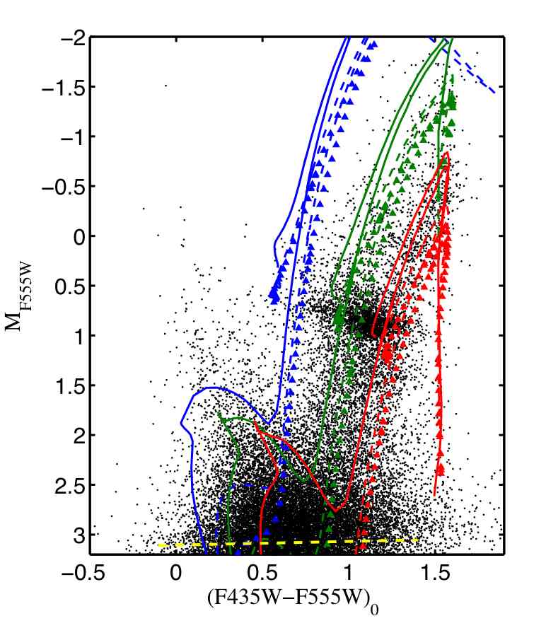
Figure 15.— CMD of M32 corrected for contamination by M31 background stars, reddening ($E(B-V)=0.08$, Burstein & Heiles, 1982), extinction ($A_{F555W}=0.25$, Sirianni et al., 2005) and distance $\mu_{0}=24.53$, which was obtained using the RCS method (see text for description). Isochrones from Marigo et al. (2008) and Girardi et al. (2008) are superimposed with metallicities of $Z$ = 0.0008,0.008, and 0.030 for ages of 2 (solid), 5 (dashed) and 9 (triangles) Gyr. Note a good match with the features that represent an intermediate-age population. Note also that the width of the RGB cannot be explained with a single metallicity and, even though a single age with a spread in metallicity could reproduce this, we cannot exclude some age spread.

Figure 12 shows that the RGB has a rather wide spread in color. Given the small (almost negligible) photometric errors at these magnitude and color levels, this cannot be explained by a single-age and -metallicity population but rather by an intrinsic large spread in the metallicity distribution. We show in Figure 15 that a population with a single age and a range of metallicities can adequately reproduce the width of the RGB. In spite of this, some age spread cannot be excluded. This is in agreement with G96 who showed that the spread in color of the M32 CMD is indicative of its metallicity range.

Figure 15 shows isochrones superimposed on the CMD of M32 corrected for reddening ($E(B-V)=0.08$, Burstein & Heiles, 1982), extinction ($A_{F555W}=0.25$, Sirianni et al., 2005) and distance $\mu_{0}=24.53$ (this paper below), that represent populations of 2 (solid lines), 5 (dashed lines) and 9 (triangles) Gyr with metallicities of $Z=$ 0.0008 (bluest), 0.008, and 0.03 (reddest). We can see that these isochrones cover the entire RGB and match the features we just discussed. However it is clear that not all of them match our data well. For example, the most metal-poor isochrones are too blue compared with our data, thus suggesting that very metal-poor stars are unlikely to be present. On the contrary, metal-rich isochrones do a better job in matching both the bright and faint end of the RGB. As stated earlier, an age-metallicity degeneracy is present in this region of the CMD, and therefore differences in ages cannot be distinguished if we look solely at the RGB.

To obtain the metallicity distribution function (MDF) of M32, shown in Figure 16, we have used isochrones from the model grid of the Padova library (Girardi et al., 2002; Marigo et al., 2008; Girardi et al., 2008) for ages of 5, 8 and 10 Gyr and $\log(Z/Z_{\odot})=\mathrm{[M/H]}$ from $-1.2$ to $0.3\,\mathrm{dex}$ with a metallicity step (bin size) of $\mathrm{[M/H]}=0.2\,\mathrm{dex}$. Although we do not see the 5 Gyr MSTO, it is possible that M32 contains such a population due to the observation of bright AGB stars that confirm the presence of an intermediate-age population (Sec. 5.1.5). For the metallicity distribution, we have first considered only RGB stars located below the RC and above the 80% completeness level, to avoid contamination by AGB stars that ascend from the RC. We selected a box containing 1166 stars of absolute magnitudes $1.2<M_{F555W}<1.8$ and dereddened colors $0.7<(F435W-F555W)_{0}<1.4$ to compute the MDF below the RC. Selecting these stars guarantees an unambiguous metallicity assignment but, even though stars in this region of the CMD have small photometric errors, they are not negligible. Figure 10 shows that at the level of apparent magnitudes $F555W\sim$ 26.5, which corresponds to an absolute magnitude of $M_{F555W}\sim 1.7$, and color $\sim 1$ the photometric errors in colors in our selected box are in between $\sim 0.05$ and $\sim 0.1$ mag. The width of the RGB at those magnitudes is $\sim 0.7$ mag and thus the small photometric errors cannot explain the observed spread in color. We also note that variations in ages, from 2 to 9 Gyr, on the RGB can only account for a $\sim 0.15$ mag variation in color (see Figure 15). On the other hand, if we use stars above the RC, for which the photometric errors are truly negligible, implying that the color variation of this region is only due to an intrinsic metallicity distribution in the populations, we need to correct for the contamination by AGB stars. We selected a box containing 500 stars of absolute magnitudes $-0.9<M_{F555W}<0.0$ and dereddened colors $0.9<(F435W-F555W)_{0}<1.65$ for the MDF above the RC.

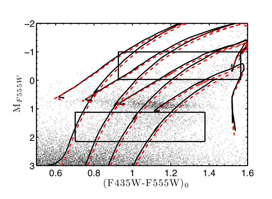
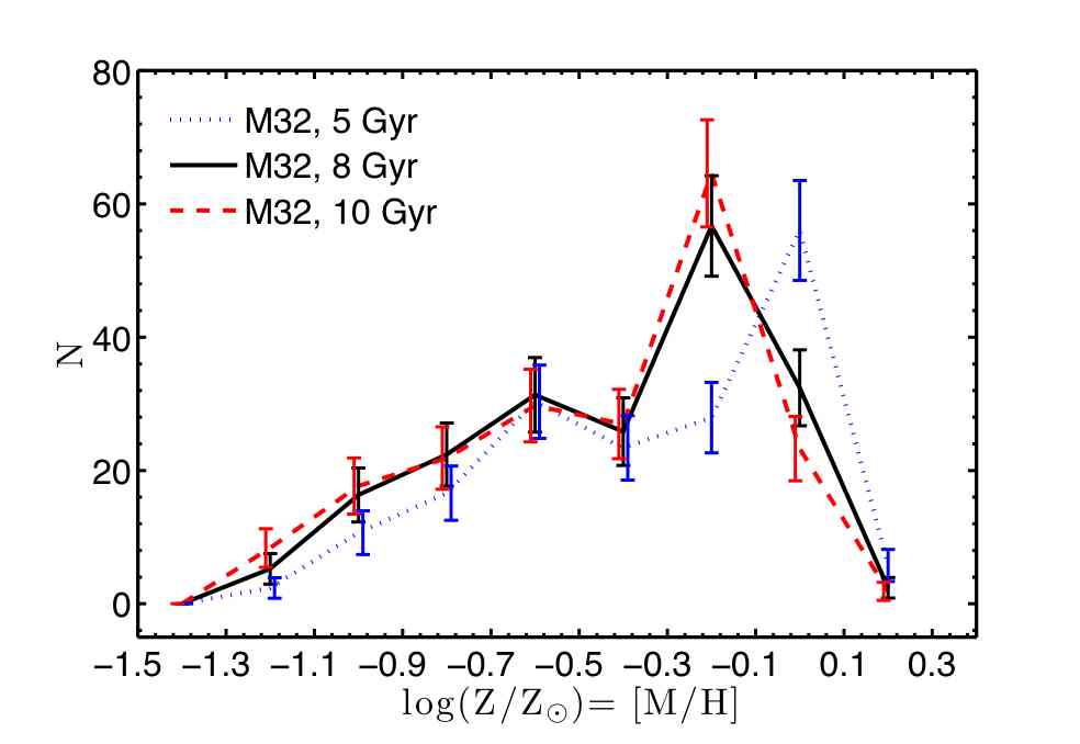
Figure 16.— Top panel Close-up of the RGB region of the decontaminated CMD of M32 (the magnitudes are de-reddened and corrected for distance). Stars inside the two boxes were used to compute the two MDFs. Black and red–dashed curves are 8 and 10 Gyr-old Girardi et al. (2008) and Marigo et al. (2008) isochrones covering a wide range in metallicity, $Z=$ 0.0012, 0.003, 0.008, 0.03. We counted stars between the isochrones of different metallicities to compute the MDF. Errors are simply Poisson errors. Middle panel MDF of M32 derived using stars above the RC, defined as the number of stars per bin size in $\log(Z/Z_{\odot})=$[Fe/H]. The counting has been corrected for contamination by AGB stars in this region. Blue, black and red lines represent 5, 8 and 10 Gyr-old MDFs, respectively. The peak of the distribution is at $\mathrm{[Fe/H]}\sim 0.0$ for 5 Gyr and is slightly more metal-poor, at $\mathrm{[Fe/H]}\sim-0.2$, for 8 and 10 Gyr-old populations. Bottom panel Same as the middle panel but considering stars below the RC, which are affected by photometric errors but not by AGB stars. Here the peak of the distribution is at $\mathrm{[Fe/H]}\sim-0.2$ for all ages. The MDF of M31 is also computed for a 10 Gyr-old population and is illustrated by the gray solid line. The M31 MDF has been normalized to the M32 MDF, and its peak is given at $\mathrm{[Fe/H]\sim-0.4}$, indicating that our background field contains more metal-poor stars. Note that the M31 metal abundance distribution looks very similar to that of M32.

We have derived a MDF for these two groups of stars. The top panel of Figure 16 shows the selected stars (boxes) and representative isochrones considered for the MDF calculation. Solid and dashed curves are the 8 and 10 Gyr isochrones, respectively. The middle and bottom panels of Figure 16 show the resulting MDF of M32 above and below the RC, respectively, defined as the number of stars per bin size in $\log(Z/Z_{\odot})$. We have counted RGB stars in the CMD between fixed-age isochrones (either 5, 8 or 10 Gyr old) covering the range of metallicities stated above. We have attempted to correct the MDF above the RC for AGB contamination by taking into account the theoretical ratio of AGB to RGB stars at different ages and metallicities. We calculated the ratio of AGB to RGB stars occupying the isochrone section considered, i.e. for a given age and metallicity, using the “int-IMF” column of Padova’s isochrones. We subtracted the corresponding number of AGB stars from the RGB counting between the isochrones considered to derive the MDF. Overall, we obtain a rather smooth distribution with many more metal-rich stars than metal-poor ones. The general peak of this distribution is given at $\mathrm{[Fe/H]}\sim-0.2\,\mathrm{dex}$ with the exception of the 5 Gyr MDF above the RC that has its peak at $\mathrm{[Fe/H]}\sim 0.0\,\mathrm{dex}$. This peak agrees with previous results (Rose, 1985, 1994; Grillmair et al., 1996b; Trager et al., 2000a; Coelho et al., 2009). We note that the peak in the MDF above the RC is more pronounced compared to that in the MDF below the RC. We believe that this arises from the cooler giant stars going back towards the blue at the TRGB due to the strong opacity present in the $V$ band.

Note that there are very few stars with metallicities $\mathrm{[Fe/H]}<-1.2$, which implies that the enrichment process largely avoided the metal poor stage (Worthey et al., 1996). Moreover, it is possible that some of the B-RGB is due to stars with ages $<2$ Gyr (see Figure 18 below), hence the number of metal-poor stars is likely to be even smaller. Note also that a few biases should have been taken into account when deriving the MDF, such as e.g. the different RGB lifetimes at different metallicities (Rood, 1972) or the rate at which stars leave the main sequence (Renzini & Buzzoni, 1986). These biases, however, mostly affect the metal-poor tail of the metallicity distribution (see Zoccali et al., 2003), which implies that our (very weak) metal-poor tail is actually an upper limit. The shape and peak of the MDF agrees very well with the photometric MDF of G96. We even obtain the same peak value, which however disagrees with the synthetic population results by Coelho et al. (2009), who found a significant amount of metal-poor stars at a location that samples the positions of both G96 and our field. Coelho et al. (2009) claim that they do not understand this difference, although they say that one might not expect an MDF derived from photometry to match an MDF derived from spectroscopic data (although see Trager et al., 2000a). Nevertheless, the difference is significant.

5.1.4 The tip of the red giant branch (TRGB)

Another important CMD feature that confirms the results obtained so far is the tip of the RGB (TRGB). This corresponds to the He-burning ignition through the He flash marking the end of the RGB phase. For very metal rich systems, such as the globular clusters NGC 6553 and NGC 6528, the TRGB in the $B$, $V$ and $R$ filters is fainter than in metal-poor systems due to the strong molecular opacities of TiO bands, which become very deep in the cool giants. This effect is so strong in the $V$ band that the TRGB in a $V$–$(B-V)$ color–magnitude diagram is accompanied by a vertical sequence of stars extending to fainter magnitudes and almost merging with the hotter giants (Ortolani et al., 1992). The location of what we identify as the TRGB in the CMD of M32, at the apparent magnitude of $F555W\sim 24$, (see Figure 12) corresponds to the theoretical predictions of a system as old as $\sim$8.5 Gyr with [Fe/H] $\sim-0.2$. This again confirms previous (e.g., G96) and our own results in this section.

5.1.5 AGB stars

Finally, the bright extension of AGB stars seen above the first-ascent red giant branch (or TRGB) is a signature of an intermediate-age population (see e.g. Freedman, 1992a; Gallart et al., 2005). We thus identify the bright stars seen in Figure 12 at apparent magnitudes $F555W<24$ and colors $1.0\lesssim(F435W-F555W)\lesssim 1.6$ as intermediate-age AGB stars. We find $\sim 130$ of these stars in the CMD of M32. To test whether blends of fainter stars could mimic bright AGBs we make use of the AST results. From AST, we considered all the recovered bright AGB stars and we looked at their injected counterpart stars, i.e. we looked at where these bright stars came from theoretically. We obtained that $\sim$ 97% correspond to the injected bright AGB. We are confident hence that the detected AGB stars in our photometry are not artifacts of crowding since they cannot be generated by blends of fainter stars. The existence of these stars confirms the results of previous studies (e.g., Freedman, 1992a; Elston & Silva, 1992; Davidge & Jensen, 2007), and strongly supports the presence of an intermediate-age population in M32. Figure 17 shows a decontaminated CMD of M32, corrected for distance and extinction with Padova solar metallicity isochrones superimposed, for ages of 1, 4, 7 and 9 Gyr. Clearly, bright AGB stars above the TRGB can be present between 1 and 7 Gyr. These bright AGB stars thus represent the evolved population resulting from star formation that occurred less than 7 Gyr ago in M32.

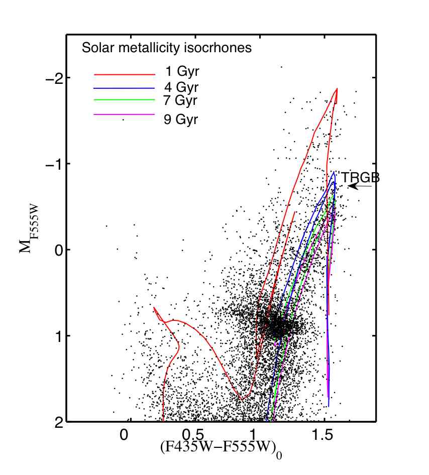
Figure 17.— CMD of M32 corrected for contamination by M31 background stars, reddening ($E(B-V)=0.08$, Burstein & Heiles, 1982), extinction ($A_{F555W}=0.25$, Sirianni et al., 2005) and distance $\mu_{0}=24.53$, obtained using the RCS method (see text for description). Isochrones from Marigo et al. (2008) and Girardi et al. (2008) are superimposed with ages of 1 (red), 4 (blue), 7 (green) and 9 (magenta) Gyr at solar metallicity. Bright AGB stars, located above the TRGB, are clearly present at ages younger than 7 Gyr.

To summarize, the RC suggests a mean age of 8–10 Gyr for a metallicity of $\mathrm{[Fe/H]}=-0.2\,\mathrm{dex}$, consistent with the position of the TRGB. The RC, RGBb and AGBb suggest a dominant population of stars with a mean age of 5–10 Gyr and a mean metallicity of $\mathrm{[Fe/H]}\gtrsim-0.4\,\mathrm{dex}$. In addition, stars younger than 7 Gyr are present as bright extended-AGB stars.

5.2. Young populations?: Ages $<$ 2 Gyr

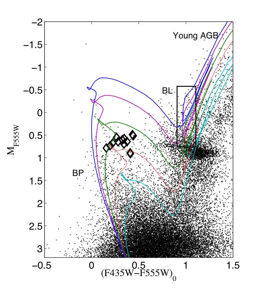
Figure 18.— CMD of M32 corrected for contamination by the M31 background stars, reddening ($E(B-V)=0.08$, Burstein & Heiles, 1982) and extinction ($A_{F555W}=0.25$, Sirianni et al., 2005). The distance modulus $\mu_{0}=24.53\pm 0.12$ was obtained using the RCS method (see text for more description). Solar metallicity isochrones from Marigo et al. (2008) are superimposed, with ages of 0.4,0.5,0.7,1, and 1.5 Gyr. Note the good fit to the extended MS of the CMD, and the suggestion of the presence of subgiant stars. On the other hand, the diamonds show the location of the RR Lyrae found in this M32 field (F10). These isochrones also fit the BL region (delineated by the black box) well, suggesting the presence of young AGB stars with masses of $2.5$–$2.8\,M_{\odot}$.

Young populations are mostly represented by stars occupying the blue plume (BP) seen in the CMD of Figure 12 at $F555W\sim 24.5$ from $F555W\sim 27$ and $(F435W-F555W)<0.5$, suggesting the presence of an extended main sequence (MS). We note that the presence of a BP in M32 has either not been claimed or not observed in previous photometric works (e.g., G96; Worthey et al., 2004). Therefore, we begin this section by addressing whether this feature is real or not. Blends of fainter blue stars could appear in our photometry as brighter blue stars, generating a BP which is actually artifact of crowding. We have tested this using the results from the ASTs. We estimated the fraction of recovered BP stars that were actually injected as red or fainter stars; $\sim$ 14% of recovered BP stars are blends, thus indicating that $\sim$ 86% are genuine blue stars. We are hence confident that the detected BP is indeed real. Moreover, we have investigated archival observations of fields near M32, which also seem to indicate the presence of a BP in M32. This analysis is shown in the Appendix.

Figure 18 shows Padova isochrones (Marigo et al., 2008; Girardi et al., 2008) for young ages superimposed on the decontaminated, de-reddened and corrected for distance M32 CMD. The isochrones have solar metallicity $\rm{Z}_{\odot}=0.019$ and a range of ages of 0.4, 0.5, 0.7, 1, and 1.5 Gyr. This suggests that M32 at F1’s location may contain stars as young as $\sim 0.5-1.5$ Gyr; other higher metallicities, for Z ranging from Z_⊙ to 0.03 ($\mathrm{[Fe/H]}\sim+0.2$), show similar results. However, lower metallicities isochrones are too blue compared with the observed data. On the other hand, we can see that any significant presence of populations younger than 0.4 Gyr is ruled out in this field, although stars as young as 0.5 Gyr may be present. We even appear to find a possible subgiant branch (SGB), with a region occupied by stars as soon as they leave the MS. These SGB stars are consistent with isochrones of ages from 0.5 Gyr to 1.5 Gyr for stars with masses $1.6-2.5$ $M_{\odot}$ and a range of metallicities $Z=0.019-0.03$ ($\mathrm{[Fe/H]}\sim 0$ to $+0.2$). We also show in Figure 18 the position of known RR Lyrae variables in field F1 (F10), indicating the presence of some blue horizontal branch stars in this region of the CMD. It is worth noting that the number of RR Lyrae discovered in this field (17, of which $7^{+4}_{-3}$ belong to M32 ) cannot account for all of the stars in this region ($\sim 100$). Nevertheless, the SGB region of the CMD is the most affected by blends: stars either bluer or redder are likely to blend and occupy this region. We tested this using the results from ASTs and found that only a $\sim 38\%$ of stars recovered in this region were actually injected there. Most of the stars are therefore blends and we are not able to assume that they are all actual SGB stars.

The presence of a blue loop (BL) is another sign of young populations and has never been detected before in M32. Stars in this region are intermediate-mass stars with ages between $\sim 0.4$ and $\sim 1$ Gyr burning helium in their cores (see, e.g., Sweigart, 1987; Xu & Li, 2004, and references therein) . Theoretical models predict that their positions strongly depend on metallicity (e.g., Girardi et al., 2000). The box in Figure 18 shows the location of BL stars. We considered the fact that these stars could also be artifacts of crowding and we analyzed this again using the results from the ASTs. We found that $\sim 80\%$ of the recovered stars in the BL region were actually injected there. We are certain that most of the stars in the BL are real and not products of blends. We can see from Figure 18 that their magnitudes and colors are consistent with the assumed solar metallicity and ages of 0.4–0.9 Gyr and they have masses in the range $\sim 2.25$—$3\,M_{\odot}$. Isochrones with lower metallicities predict the location of the BL bluer than observed. Note also that the isochrones in Figure 18 suggest the presence of young AGB stars as well, of ages between 0.7–1 Gyr, with masses of 2.5–$2.8\,M_{\odot}$. However this region may be also occupied by older RGB and AGB stars with lower metallicities (see the previous section) and much lower masses, of the order of $0.9$–$1\,M_{\odot}$.

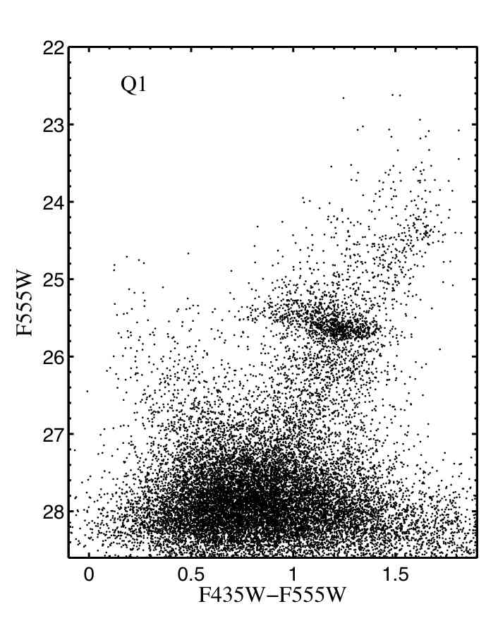
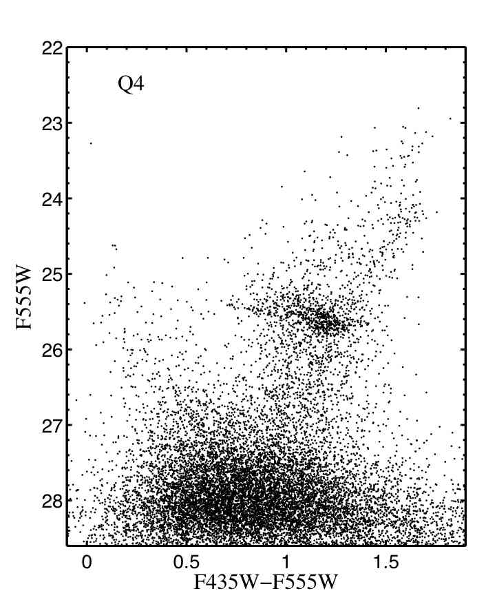
Figure 19.— Left panel: CMD of the quadrant Q1 closest to the nucleus of M32 in F1. Right panel: CMD of the quadrant Q4 furthest away from the nucleus of M32. We compare the BP in these two CMDs in order to test whether it belongs to M32 or it represents a constant M31 background in F1. It seems that the fainter BP $F555W>26$ is indeed stronger in Q1, which indicates that this portion of the BP comes from M32. However, the brighter BP stars, which assured the presence of a young population, do not show any significant difference between the two CMDs. They could represent a constant M31 disk background in F1. See text and Table 4 for more information.

Table 4Star counts in different boxes of the CMDs. Regions are indicated as in Figure 12

CMD Region	F1	F2	Q1F1	Q4F1	F1$-$F2	Q1${}_{\rm{F1}}-$ Q4F1	F1/F2
BP stars
$24.0<F555W<25.5$	$\phantom{0}\phantom{0}93~{}\pm~{}10$	$\phantom{0}\phantom{0}64~{}\pm~{}\phantom{0}8$	$\phantom{0}\phantom{0}22~{}\pm~{}\phantom{0}5$	$\phantom{0}\phantom{0}27~{}\pm~{}\phantom{0}5$	$\phantom{0}\phantom{0}29~{}\pm~{}13$	$\phantom{0}\phantom{0}-5~{}\pm~{}\phantom{0}7$	$1.45~{}\pm~{}0.24$
$25.5<F555W<26.0$	$\phantom{0}169~{}\pm~{}13$	$\phantom{0}\phantom{0}80~{}\pm~{}\phantom{0}9$	$\phantom{0}\phantom{0}48~{}\pm~{}\phantom{0}7$	$\phantom{0}\phantom{0}45~{}\pm~{}\phantom{0}7$	$\phantom{0}\phantom{0}89~{}\pm~{}16$	$\phantom{0}\phantom{0}\phantom{0}3~{}\pm~{}10$	$2.11~{}\pm~{}0.29$
$26.0<F555W<27.0$	$1477~{}\pm~{}38$	$\phantom{0}534~{}\pm~{}23$	$\phantom{0}451~{}\pm~{}21$	$\phantom{0}336~{}\pm~{}18$	$\phantom{0}943~{}\pm~{}44$	$\phantom{0}115~{}\pm~{}27$	$2.76~{}\pm~{}0.14$
BL stars
$23.5<F555W<25.2$	$\phantom{0}263~{}\pm~{}16$	$\phantom{0}127~{}\pm~{}11$	$\phantom{0}\phantom{0}70~{}\pm~{}\phantom{0}8$	$\phantom{0}\phantom{0}64~{}\pm~{}\phantom{0}8$	$\phantom{0}136~{}\pm~{}20$	$\phantom{0}\phantom{0}\phantom{0}6~{}\pm~{}11$	$2.07~{}\pm~{}0.22$
Bright AGB
$22.0<F555W<24.0$	$\phantom{0}211~{}\pm~{}14$	$\phantom{0}101~{}\pm~{}10$	$\phantom{0}\phantom{0}64~{}\pm~{}\phantom{0}8$	$\phantom{0}\phantom{0}55~{}\pm~{}\phantom{0}7$	$\phantom{0}\phantom{0}110~{}\pm~{}17$	$\phantom{0}\phantom{0}\phantom{0}9~{}\pm~{}10$	$2.09~{}\pm~{}0.25$
RGB
$24.0<F555W<25.2$	$1205~{}\pm~{}35$	$\phantom{0}372~{}\pm~{}19$	$\phantom{0}358~{}\pm~{}19$	$\phantom{0}268~{}\pm~{}16$	$\phantom{0}833~{}\pm~{}40$	$\phantom{0}\phantom{0}90~{}\pm~{}25$	$3.24~{}\pm~{}0.19$
$25.2<F555W<26.0$	$3998~{}\pm~{}63$	$1243~{}\pm~{}35$	$1174~{}\pm~{}34$	$\phantom{0}894~{}\pm~{}30$	$2755~{}\pm~{}72$	$\phantom{0}280~{}\pm~{}45$	$3.22~{}\pm~{}0.10$
$26.0<F555W<26.8$	$2857~{}\pm~{}53$	$\phantom{0}953~{}\pm~{}31$	$\phantom{0}876~{}\pm~{}30$	$\phantom{0}631~{}\pm~{}25$	$1904~{}\pm~{}61$	$\phantom{0}245~{}\pm~{}40$	$3.01~{}\pm~{}0.11$

The bright stars composing the BP and BL features remain in the CMD even after the statistical decontamination for M31 stars. This would indicate that they belong to M32. However, while we took care to characterize the M31 disk ground by devoting equal time to the F2 images, the surface density of the M31 disk may (unfortunately) be higher at F1 than it is at F2. Arp (1966) noted that M32 (Arp 168) appears to have a diffuse “plume” of emission to the south of its nucleus, and thus in the direction of F1. Choi et al. (2002) attempted to isolate this feature through a variety of surface photometry models, and suggested that it is due to the tidal interaction of M31 with M32. The obvious inference is that the plume comprises stars that have been stripped from M32; however, if the plume instead represents material drawn for the M31 disk, then this may enhance the contribution of disk stars to F1 over what we would have inferred from F2. To test whether the young population (ages $<$ 1 Gyr) comes from M32 or M31, we have first compared the CMDs obtained from closest and furthest quadrants from the nucleus of M32 (hereafter Q1 and Q4, respectively) in F1. Since, given the rapid decline of the M32 surface brightness, we observe a gradient in the stellar density of M32 over F1 (Figure 2), we should therefore detect a larger number of bright BP and BL stars as we approach the nucleus of M32 if they belong to M32. Figure 19 shows the CMDs in apparent magnitudes obtained in Q1 (left panel) and in Q4 (right panel). The number of BL stars as well as BP stars brighter than $F555W\sim 26$ seems to be roughly the same in both CMDs. However, the number of fainter BP stars ($F555W>26$) is significantly larger in Q1. To quantify this, we define eight boxes in different regions of the CMDs and we count stars in them. The different regions are the BP, BL, AGB and RGB (see Figure 12) and the corresponding boxes are indicated in Table 4. This analysis was done not only in the Q1 and the Q4 CMDs but also in the F1 (before decontamination for F2) and F2 CMDs. Assuming Poisson statistics we can infer whether (F1$-$F2) and/or (Q1$-$Q4) is significantly positive for each of the boxes. The results of (Q1$-$Q4) suggest that there is a constant background of bright blue stars over F1, since there is no significant difference between the number of bright BP and BL stars. The ratio between the number of stars in F1 to F2 is also shown in Table  4 for each of the regions. This fraction is expected to be $\sim$ 3 according to the surface brightness estimates at F1’s location. Note that this is clearly the case for the RGB stars and the fainter BP stars ($26.0<F555W<27.0$). However, the ratio is lower than 3 for the brighter portion of the BP, the BL and bright AGB stars which indicates that the M31’s background is relatively enhanced in F1 compared to what F2 represents. As stated above, a plausible explanation for an enhanced contribution of disk stars to F1 is that the “diffuse plume” observed in M32 at F1’s location (Arp, 1966) represents material drawn for the M31 disk. Given the null difference between stars in Q1 and Q4, it is likely that all of the bright BP stars belong to M31. It is likely then that the very young population that we see in the decontaminated CMD of M32 (i.e. stars with ages $\sim 0.5$ Gyr) belongs to the disk of M31 rather than to M32. Instead, stars in the BP at magnitudes $F555W>26$ do belong to M32 and represent a population of ages between 1 and 2 Gyr (see Figure 18). Further investigation is required to conclusively determine whether a young population of stars with ages $\sim 0.5$ Gyr do or do not belong to M32. Wide field images from fields closer to the nucleus of M32, as could be obtained with HST/WFPC3, would reveal this. Note that the Q1$-$Q4 difference in the bright AGB region is positive, and the F1/F2 ratio for these stars is significantly higher than for the brightest BP stars. This implies that, even though there is an enhancement of M31 AGB stars over what F2 represents, it is likely that a fraction of them still belong to M32.

Young population vs. Blue straggler stars

Blue straggler stars (BSSs) are stars hotter, bluer and brighter than the MSTOs in a CMD and thus generate a blue plume, similar to the one we see in the CMD. As they can mimic a young population (ages $<~{}$2 Gyr), it is crucial for the derivation of the SFH to understand whether the BP we find in M32 is entirely populated by old BSSs instead of a genuinely young population.

BSSs have been seen in globular and open clusters (e.g., Ferraro et al., 2004; Mapelli et al., 2004, 2006; Piotto et al., 2004; de Marchi et al., 2006) where there is no recent star formation or the spread in stellar age is small enough such that their identification as old BSSs (instead of as a young population) is very clear. In a field population it is difficult to unambiguously prove the nature of the BP as old BSSs (see, e.g., Mateo et al., 1995; Hurley-Keller et al., 1999; Aparicio et al., 2001; Carrera et al., 2002; Mapelli et al., 2009). Only Momany et al. (2007) in their work indicated that their BSS candidates in dSphs may be real BSSs. They found a statistically-significant anti-correlation between the specific frequency of BSS candidates with the HB stars and the absolute magnitude of their dSph sample, similar to what has been observed in both globular clusters (Piotto et al., 2004) and open clusters (de Marchi et al., 2006). Momany et al. (2007) claimed that this anti-correlation can be used as a classification tool such that galaxies following the anti-correlation are more likely to have real BSSs rather than young MS stars (the anti-correlation would be hard to explain if BSS candidates were young stars). It is worth of mentioning that they selected their sample in such a way that dwarf spheroidals/irregulars in which there is current or recent ($\leq 500$ Myr) star formation were not considered. Therefore, an ideal test for our data would be to calculate the frequency of BSS candidates in M32 and compare our results to the proposed relation of Figure 2 of Momany et al. (2007). However, the box considered to include the candidates of old BSSs goes from the magnitudes of the oldest MSTOs up to where there are blue stars observed. We do not reach the oldest MSTOs; the stars at the appropriate magnitude level are dominantly products of blends, which will contaminate the BSS candidates in our data. We are therefore unable to test, at least in this way, whether the BP consists of old BSSs. Nevertheless, we favor the idea that the BP cannot be entirely populated by old BSSs but instead contains some genuine young stars due to the following: Brown et al. (2006) argue that, even though the formation mechanism of BSS is not completely understood, BSSs in an old population will be limited to $M<2M_{\sun}$, whereas the masses required to explain stars as bright as, and even exceeding, the HB luminosity level that we see in our CMD are higher than that value ($2<\rm{M}<3\rm{M_{\odot}}$). This implies that at least the brightest BP stars observed are truly young stars. However, as explained above, they are likely to belong to the disk of M31 rather than to M32. The fainter BP, $F555W>26$, associated to M32 is not assured to be only young stars and it could even be composed only of BSSs.

5.3. Ancient population: Ages $>$ 10 Gyr

We believe that old and metal-poor stars should be present in M32, since previous generations of stars are required to produce the metal-rich population we observe. It is clear from our CMD that there are not many of these stars since there is no noticeable presence of blue horizontal branch (BHB) stars. Therefore a well-developed old, metal poor population is not present. Nonetheless, RR Lyrae variable stars were found in our M32 field with our data (F10), revealing the presence of BHB stars. The pioneering work of Brown et al. (2000, 2008) showed evidence of extreme horizontal branch (EHB) stars in the central region of M32 from Space Telescope Imaging Spectrograph (STIS) UV observations. By detecting RR Lyrae stars in our data, we find a different manifestation of a consistent picture.

The RR Lyrae stars found with the data from this study have a mean metallicity of $\mathrm{\langle[Fe/H]\rangle}\sim-1.5$ (F10). Taking into account the metallicity distribution we have obtained (see above) and assuming that these metal-poor stars are ancient stars, we can estimate the fraction of these stars in our data. We find that, when assuming a 10 Gyr-old population, metal-poor stars with $\mathrm{[Fe/H]}\leq-1$ represent at most $\sim$ 5.7% of the total $V$-band light in our M32 field (recall that the number of stars in metal-poor tail of the MDF is an upper limit). Worthey (1994) models can be used to obtain the stellar M/L ratio for different metallicities at a given assumed age. We estimate that a metal-poor 10 Gyr-old population contributes $\sim$ 4.5% of the total mass in our observed field. Note however that there is little constraint on ancient, metal-rich populations. The fact that the hot HB stars do not significantly contribute to the optical $V$-band light of M32 suggests that the strong Balmer lines found in spectroscopic studies (O’Connell, 1980; Pickles, 1985; Bica et al., 1990; Rose, 1994) actually represent a young population or BSSs. Trager et al. (2000b) estimated that the BHBs needed to account for the strong Balmer lines of M32 ($\mathrm{H}\beta=1.9$ Å, corresponding to an integrated light age of $\sim$ 8 Gyr) at F1’s location would contribute to the $\sim$ 5% of the $V$-band light. This would imply that $\sim$ 25% of the total light would have to come from metal-poor stars, which is $\sim$5 times more than the amount of metal-poor $V$-band light that we have found. On the other hand, to explain the high-$\mathrm{H}\beta$ strength of M32 arising from a population of BSSs would require that $\gtrsim 15\%$ of the $V$-band light come from BSSs (Trager et al., 2000a). This will be explored in a follow-up paper where the derived SFH will allow us to quantify the light contribution of the BP in F1.

5.4. The Luminosity function of M32

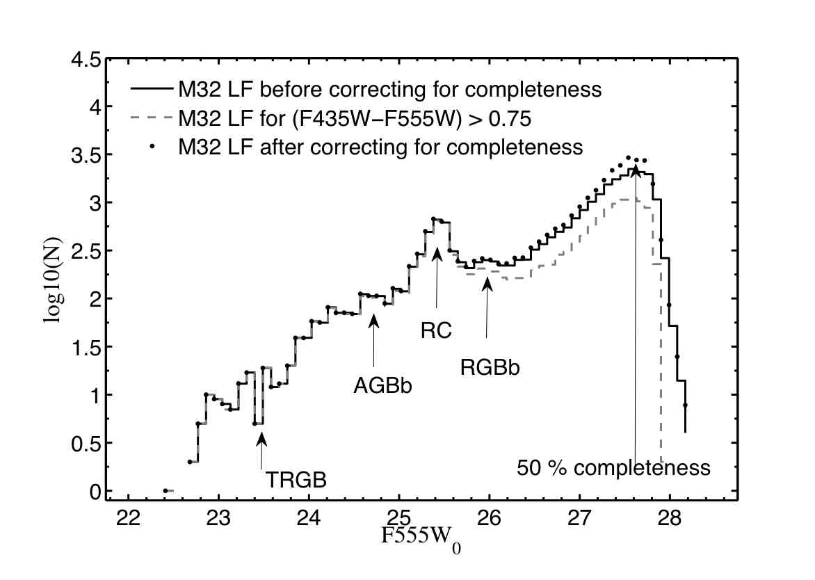
Figure 20.— $F555W_{0}$-band Luminosity Function (LF) for M32, corrected for extinction and decontaminated for M31 background stars, is shown in the solid histogram. The completeness-corrected LF is shown as black dots. The gray-dashed line shows the LF for stars redder than $(F435W-F555W)\sim 0.75$ to avoid contamination from, for example, the BP. The 50% completeness level is indicated at a magnitude of $F555W_{0}\sim 27.75$. The main features of this LF are indicated by arrows. The TRGB lies at $F555W_{0}\sim 23.7$, the AGB bump at $F555W_{0}\sim 24.7$, the RC at $F555W_{0}\sim 25.4$, and the RGB bump at $F555W_{0}\sim 25.9$.

Table 5M32 Luminosity Function

$F555W_{0}$	$N$	$N_{corr}$	$N_{(col>0.75)}$	$F555W_{0}$	$N$	$N_{corr}$	$N_{(col>0.75)}$	$F555W_{0}$	$N$	$N_{corr}$	$N_{(col>0.75)}$
22.45	1	1.00	1	24.44	73	73.64	51	26.43	257	276.43	135
22.53	0	0.00	0	24.52	77	77.55	66	26.51	329	349.93	138
22.62	0	0.00	0	24.60	107	107.77	61	26.59	366	389.89	143
22.70	2	2.00	2	24.69	91	91.94	86	26.67	418	453.06	150
22.78	9	9.00	2	24.77	96	97.35	91	26.76	480	526.73	196
22.87	6	6.00	11	24.85	79	79.40	89	26.84	517	568.22	192
22.95	8	8.00	7	24.94	119	120.55	86	26.92	652	721.45	188
23.03	8	8.00	8	25.02	110	111.61	77	27.01	751	852.73	251
23.11	8	8.00	3	25.10	191	194.20	103	27.09	929	1052.41	267
23.20	12	12.08	10	25.18	257	261.86	100	27.17	1106	1277.55	312
23.28	10	10.00	10	25.27	400	409.63	170	27.25	1356	1598.82	356
23.36	13	13.00	16	25.35	534	544.64	210	27.34	1586	1896.35	433
23.45	14	14.00	6	25.43	628	641.55	339	27.42	1671	2072.59	535
23.53	5	5.00	15	25.52	433	445.35	456	27.50	1936	2462.01	608
23.61	16	16.00	4	25.60	235	242.03	601	27.59	2009	2633.19	775
23.69	15	15.00	17	25.68	203	211.08	466	27.67	1885	2519.17	844
23.78	21	21.00	14	25.76	201	208.43	232	27.75	1626	2260.72	907
23.86	33	33.00	18	25.85	220	228.30	190	27.83	740	1075.84	977
23.94	36	36.11	33	25.93	235	247.53	146	27.92	179	276.44	891
24.02	56	56.39	32	26.01	229	239.49	173	28.00	44	72.50	872
24.11	50	50.00	53	26.09	200	209.56	183	28.08	12	21.28	623
24.19	68	68.00	46	26.18	196	205.74	171	28.16	4	7.77	113
24.27	67	67.12	57	26.26	230	243.67	170
24.36	64	64.11	70	26.34	234	247.77	139

The extinction-corrected $F555W_{0}$ luminosity function (LF) for M32 is given in Table 5. The LF is measured by dividing the $F555W_{0}$ magnitudes into 65 bins with a bin width of $\Delta F555W_{0}=0.1$ mag. The LF is shown as the solid histogram in Figure 20. We have also calculated the completeness-corrected LF (black dots). The long vertical arrow marks the 50% completeness level at $F555W_{0}\sim 27.75$. The main distinct features are indicated by arrows: the TRGB at $F555W_{0}\sim 23.7$, the AGBb at $F555W_{0}\sim 24.7$, the RC at $F555W_{0}\sim 25.4$ and the RGBb at $F555W_{0}\sim 25.9$. These features are consistent with the CMD analysis above. We also show the LF for stars redder than $(F435W-F555W)=0.75$, as gray-dashed histogram. We can see that the features that we find on the RGB region, in particular the RGBb, are better identified when we plot only the redder stars thus avoiding contamination from, for example, the BP.

To summarize this section, M32 is dominated by a 8–10 Gyr old, metal-rich ($[\mathrm{Fe/H}]=-0.20\,\mathrm{dex}$) population, due to the RC location and width of the RGB. This result is supported by the locations of the RGBb and the AGBb. Intermediate-age stars of $4\pm 3$ Gyr are also present in M32, as revealed by the bright AGB stars observed and the morphology of the strong RC. We see evidence for 1–2 Gyr MSTO stars and/or BSSs due to the presence of the BP. An ancient metal-poor population does not contribute much to the light of M32 in F1. There is, however, little constraint on its metal-rich counterpart.

6. The Distance to M32 and M31

We determine the distance to M32 using the Red Clump Stars (RCS). Udalski (1998) has stressed that this method has many advantages with respect to other widely used standard candles such as Cepheid and RR Lyrae: for example, RCS are easy to recognize in a CMD and large samples are usually present in galaxies, which is certainly true in our case. Another important advantage is the fact that the mean absolute magnitude of RCS in the Solar neighborhood has been calibrated by Hipparcos (Perryman & ESA, 1997; Perryman et al., 1997) parallaxes with an accuracy of 10%. The disadvantage however is that its properties are not the same for all galaxies, given the age-metallicity dependence of the RC which affects the value of its absolute magnitude. Since models of core-helium-burning stars predict that the RC luminosity depends on both age and metallicity (Cole, 1998; Girardi et al., 1998; Girardi & Salaris, 2001), “population corrections” to the RC absolute magnitude obtained using Hipparcos parallaxes need to be made before it can be used as an accurate extragalactic distance indicator. Percival & Salaris (2003) have calculated how the absolute magnitudes of RCS differ for a given age and metallicity when compared with the Solar-neighborhood RC absolute magnitude, $\Delta M^{\mathrm{RC}}_{\lambda}$. Taking these variations into account, we can still use the RCS to estimate the distance of M32. The true distance modulus of the galaxy will be given by

$$\mu_{0}=(m-M)_{0}=m^{\mathrm{RC}}_{\lambda}-M^{\mathrm{RC}}_{\lambda,\mathrm{local}}-A_{m_{\lambda}}+\Delta M^{\mathrm{RC}}_{\lambda},$$ (7)

where

$$\Delta M^{\mathrm{RC}}_{\lambda}=M^{\mathrm{RC,theory}}_{\lambda,\mathrm{local}}-M^{\mathrm{RC,theory}}_{\lambda,\mathrm{galaxy}}.$$ (8)

The mean apparent magnitude of RC calculated in section 5.1.1 above is $F555W=25.66\pm 0.082$. This value is then de-reddened assuming $E(B-V)=0.08$ (Burstein & Heiles, 1982) and an extinction of $A_{F555W}=0.25$ (Sirianni et al., 2005). On the other hand, the Hipparcos absolute magnitude and the theoretical population corrections to the Red Clump absolute magnitudes were calibrated and calculated on the UBV system. We need therefore to transform our data from the ACS/HRC VEGA system $F435W$ and $F555W$ to the ground-based $B$ and $V$ magnitudes. We use the Sirianni et al. (2005) transformations for this. The $M_{V}^{\mathrm{RC}}$ from Hipparcos for the solar neighborhood is calibrated as $M^{\mathrm{RC}}_{V,\mathrm{local}}=0.73\pm 0.03$ (Alves et al., 2002). The population correction $\Delta M^{\mathrm{RC}}_{\lambda}$ is calculated by Percival & Salaris (2003) and we refer to that paper for a detailed explanation. Briefly, to study the age and metallicity dependence of the RC brightness, they compare their empirically derived population corrections with the theoretical models of Girardi et al. (2000, see Figure 2 in Percival & Salaris 2003). In our case, assuming an average $\langle[\mathrm{Fe/H}]\rangle=-0.2\,\mathrm{dex}$ and an age of 8 Gyr for our RCS (G96, this paper), $\Delta M^{\mathrm{RC}}_{V}=-0.1$. Percival & Salaris (2003) calculate the residuals of $\Delta M^{\mathrm{RC}}_{\lambda}$ for their model – observed fits taking into account both the metallicity and age residuals. The mean residual in $\Delta M^{\mathrm{RC}}_{V}$ is $+0.03\pm 0.07$, where the error is the $1\sigma$ error. The true distance modulus of M32 from Equation 7 is therefore

$$\mu_{0}=(25.33\pm 0.088)-(0.73\pm 0.03)+(-0.10+0.03\pm 0.07)$$ (9)

or

$$\mu_{0}(\rm{M32})=24.53\pm 0.12$$ (10)

in agreement with previous results, e.g. $24.2\pm 0.3$ (Freedman, 1992b), $24.55\pm 0.08$ (Tonry et al., 2001), $24.39\pm 0.08$ (Jensen et al., 2003), and $24.53\pm 0.21$ (F10).

We can also obtain the distance to M31 from our background field using the RCS of F2. This will also give us a relative distance measurement between these two galaxies. To this end, we selected 1107 stars from field F2 having apparent magnitudes $25.0<F555W<26.0$ and colors $0.95<(F435W-F555W)<1.32$. We then fit the histogram of the luminosities and colors of these stars with Equation 6. We find $F555W_{m}=25.49\pm 0.06$ and $(F435W-F555W)(RC)=1.14\pm 0.10$. After we de-redden ($E(B-V)=0.08$) and transform these values onto the UBV system (Sirianni et al., 2005), we consider the differences between the mean RC population in M31 at our field location and the RCS in our solar neighborhood. We consider the metallicity $[\mathrm{Fe/H}]=-0.40\,\mathrm{dex}$ and an age of 8 Gyr for our M31 field, which corresponds to a population correction $\Delta M^{\mathrm{RC}}_{V}=+0.02$ (Percival & Salaris, 2003). We obtain a true distance modulus of

$$\mu_{0}(\rm{M31})=24.45\pm 0.14$$ (11)

for M31, in agreement with previous estimates of its true distance modulus, e.g. $24.44\pm 0.11$ (Freedman & Madore, 1990), $24.50\pm 0.10$ (Brown et al., 2004), and $24.47\pm 0.07$ (McConnachie et al., 2005). The most up-to-date values have been obtained using Cepheids (Saha et al., 2006) and RR Lyrae (Sarajedini et al., 2009; Fiorentino et al., 2010), $\mu_{0}=24.54\pm 0.07$, $24.46\pm 0.11$, and $24.49\pm 0.19$, respectively. Clearly the obtained values here for M32 and M31 distance moduli are comparable, and, within the errors, it is not possible to determine with our data whether M32 is projected in front of or behind M31. We are therefore unable to confirm the results of Ford et al. (1978), who found evidence of M32 being in front of M31.

7. M31 stellar populations in F2

Field F2 serves not only as a background, allowing the M32 photometry to be decontaminated for M31, but is also very important as it contains information about the stellar populations in the inner disk and bulge of M31. In this section we first compare the stellar populations in F2 with the ones in F1. We then analyze the M31 stellar population from the F2 CMD and compare it with what it is known in the literature.

7.1. Differentiating the F1 and F2 CMDs

The CMDs of F1 and F2 are shown in Figure 7. We note that, at first glance, they are very similar. They seem to share the same morphology: a wide RGB, a noticeable RC, and a BP. Furthermore, when we statistically subtract field F2 from F1, we notice that many features remain in the CMD of M32. Thus, due to the similarities in both CMDs, we cannot be certain there is not M32 contamination in field F2. Is it possible that F2 field is contaminated with tidal debris from M32? If there were M32 contamination in the background field, we have overcorrected the M32 CMD and we are thus missing information about our primary field F1. Note that this is unlikely: the predicted contribution of M32 to the F2 field is very small, representing a surface brightness of $\mu_{V}\approx 27.5$, while M31 has $\mu_{V}\approx 22.7$ in this field. On the other hand, we want to be sure that the contamination from M31 was completely removed from F1 (statistically speaking), and not under-subtracted.

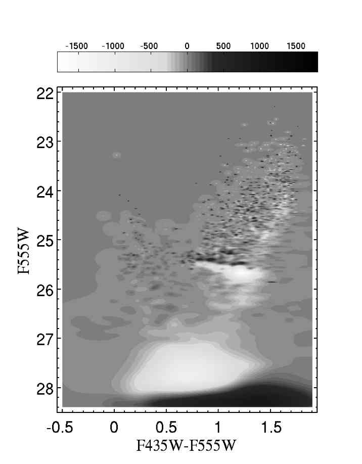
Figure 21.— Subtraction of the normalized F1 error-based Hess diagram from the F2 one. The normalization is such that the number of stars in F1 and F2 are the same. The normalization factor is 0.32. Negative values imply over-subtraction and therefore more M32 stars, and positive ones represent under-subtraction and therefore more M31 stars. The subtraction reveals significant morphological differences between the M32 and M31 background CMDs.

To investigate whether there are differences in the morphology of these two CMDs, which then would reveal differences in the stellar populations, we have subtracted the normalized F1 Hess diagram (before decontamination) from the F2 one. The F1 Hess diagram has been normalized by a factor of 0.32, which is the ratio of the F2 to F1 (uncorrected for M31 contamination) stars above the 80% completeness level. The F2 Hess diagram has been also normalized by its total number of stars above a completeness level of 80%. Thus, both diagrams are normalized so that they have the same amount of stars. Figure 21 shows the result of this subtraction. Negative values illustrate over-subtraction (more M32) whereas positive values represent under-subtraction (more M31).

Interestingly the subtraction exposes clear differences between the two CMDs. An over-subtraction would imply an excess of the relative fraction of M32 stars in that region of the CMD. On the contrary an under-subtracted region would imply an excess of fraction of M31 stars. It is clear from the subtraction that the RC in the M31 field lies at and extends towards bluer colors, indicating a more metal-poor population than in M32. In addition, the RGB of M32 is considerably redder than that of M31, indicating higher metallicity stars in M32 not present in M31. There is not a significant difference in the BP population. However there appears to be an excess of F2 stars at higher luminosities, in the BP, indicating a larger number of stars with younger ages present in M31. The fraction of M32 stars in the region of apparent magnitudes F555W between $\sim 27$ and $\sim 28$ dominates over M31 stars (see Table 4). This, together with the different morphologies of the RCs, suggests that M32 possesses more intermediate age stars than M31 in our fields. Note in addition that there is a magnitude difference, $\sim 0.2$ mag, between the RCs in F1 and F2. The brighter RC in M31, however, does not directly indicate that M32 must be behind M31. As stated in previous sections (see, e.g., Sections 5.1 and 6), the CMD location of the RC for a stellar system depends on both its age and metallicity. Hence, a difference between the RC’s magnitudes in F1 and F2 CMDs may be only due to differences between the stellar populations of M32 and M31.

Overall, this subtraction reveals that the M31 stellar populations in our field F2 are younger and more metal-poor than the M32 population in F1. The latter is in agreement with the MDFs.

7.2. M31 inner disk and bulge stellar populations

The stellar populations of the disk of M31 have been extensively studied by several means. However, those studies were mainly focused on the outer disk of M31. The present data are the deepest optical observations of the inner disk of M31 to date and are sensitive to the young stellar populations.

We summarize here our findings about the stellar populations in F2. The broad RGB of its CMD (right panel in Figure 7) indicates a wide metallicity spread. We derive the MDF of M31, using the method of Section 5.1.3, and it is shown in the bottom panel of Figure 16 as a gray line representing a 10 Gyr-old population. The F2 histogram has been multiplied by a factor of 1.9, the ratio of the decontaminated M32 to field F2 stars with completeness level above 80%. The selection of stars to compute the MDF has the same constraints as in the M32 MDF computation but only the results for stars below the RC are shown here since there was no difference with those above the RC. We have selected 611 stars below the RC in F2, having absolute magnitudes $0.95<M_{F555W}<1.60$ and dereddened colors $0.75<(F435W-F555W)_{0}<1.40$. We have assumed a Galactic reddening of $E(B-V)=0.08$ (Burstein & Heiles, 1982) and a distance modulus for M31 of $\mu_{0}(\rm{M31})=24.45$ (this paper). The peak of this distribution is at $[\mathrm{Fe/H}]\sim-0.4\,\mathrm{dex}$, indicating a more metal-poor population of stars in our background field than in F1. Note that almost no stars more metal-poor than $[\mathrm{Fe/H}]\sim-1.2\,\mathrm{dex}$ are present in our data. We detect blue stars above the HB level, indicating the presence of stars as young as 0.5 Gyr (see argument in Brown et al. 2006 and in Section 5.2 above). The detection of AGB stars indicates the presence of an intermediate-age population. However, the Hess diagram subtraction suggests that this population in our M31 field is less significant than that in M32 (see Figure 21).

Williams (2002) studied 27 fields in the disk of M31, using HST/WFPC2 archival data. He performed photometry on these fields and statistically derived the star formation history of each of them. The random distribution of most of these fields as well as the comparison of their SFHs allow an overall understanding of the formation and evolution of the M31 disk. Note, however, that these data are strictly limited to the giant branch and, therefore, an accurate measurement of the age cannot be achieved. Williams concluded that the SFR of the disk as a whole has been very active until about 1 Gyr ago, when the overall SFR declined with the exceptions of some areas of the spiral arms. He also showed that the disk of M31 is deficient in old metal-poor stars and that an intermediate-age, metal-rich population is present in most of the fields. A young population, however, is only significant in fields within the spiral arms. From the 27 fields, three are located in the vicinity of M32 which show nearly identical SFRs. Their SFRs indicate a moderate decline from 10 Gyr to 1 Gyr followed by a steep decline after that. The metallicity of these three fields is quite high, $[\mathrm{Fe/H}]>-0.5~{}\text{dex}$, with only a very small fraction of stars with $[\mathrm{Fe/H}]\sim-1.0~{}\text{dex}$ in one of the fields. Worthey et al. (2005) have also studied archival observations of HST/WFPC2 fields in the disk of M31. They however restricted their interest to the metal abundance distribution and the efficacy of the closed-box model. They find a robust metal abundance distribution that appears to hold in the vicinity of our fields but also further out, with a FWHM of $\sim 0.6\,\mathrm{dex}$. The peak of the distribution at $[\mathrm{Fe/H}]=-0.25\,\mathrm{dex}$ is quite metal-rich, which agrees with Williams’ results. Olsen et al. (2006), on the other hand, studied high resolution, deep near-IR images of the inner disk and bulge of M31 obtained with Gemini North telescope. They conclude that most of the inner disk and spheroid are indistinguishably old, with stellar populations dominated by median ages larger than 6 Gyr. They find a metallicity of $[\mathrm{Fe/H}]\sim-0.7\,\mathrm{dex}$ in the disk, in agreement with Ferguson & Johnson (2001). Interestingly, their outermost disk fields, which are comparable in radial distance to our field F2, have a 10% population of 1 Gyr or younger stars, more young stars than in their inner fields.

The most extensive study about the disk of M31 was done by Brown et al. (2006). They used deep HST ACS observations of three fields in M31, one located on the disk at $\sim 25$ kpc from the center of the galaxy, one in the spheroid, and one tidal stream field. Their data reach stars well below the oldest MSTO, which allowed them to derive the complete star formation history in those fields. Regarding the outer disk field, they found a broad RGB, which suggests a wide range of metallicity. They failed to find a significant old metal-poor population in the disk of M31, due to the small amount of blue HB stars. The detection of a BP indicates that there is at least some very young population, with ages of 0.2 – 1 Gyr, in agreement with Olsen et al. (2006). After quantitatively fitting their CMDs, Brown et al. concluded that the outer disk population is dominated by stars of 4–8 Gyr, with a mean age of 7.5 Gyr and a mean metallicity of $\text{[Fe/H]}=-0.2~{}\text{dex}$. If the contamination from their spheroid field population is taken into account, they found a younger mean age (6.6 Gyr) and a higher mean metallicity ($\text{[Fe/H]}=+0.1~{}\text{dex}$). Thus the spheroid contamination almost completely accounts for the old and metal-poor stars in the outer disk. Note, however, that given the wide separation between their fields, they cannot be assured that their spheroidal field is representative of the underlying spheroid in the disk field.

In general, the stellar populations we find in F2 agree with previous studies of M31. In particular, the MDF that we have obtained for M31 agrees very well with the findings by Williams (2002), with a peak at $[\mathrm{Fe/H}]>-0.5~{}\text{dex}$ and devoid of stars with metallicities lower than $[\mathrm{Fe/H}]\sim-1.0~{}\text{dex}$. The lack of a significant amount of metal-poor stars is a common property found in all the studies just discussed. Our metallicity peak is, however, slightly more metal-poor than that obtained by Worthey et al. (2005) and Brown et al. (2006), and slightly more metal-rich than the value obtained by Olsen et al. (2006). Hence, the possibility raised above that field F2 contains stripped M32 stars is unlikely. A more quantitative study of the stellar populations in F2 will be presented in a follow-up paper.

8. Summary

Deep $F435W$ ($\sim B$), $F555W$ ($\sim V$) observations of two fields located at $\sim 110\arcsec$ (M32 field F1) and $\sim 320\arcsec$ (M31 background field F2) from the nucleus of M32 were made using ACS/HRC on board HST. The location of the M32 field was chosen so that both the image crowding and contamination from M31 disk were as minimal as possible. The M31 background field was located at the same M31 isophotal level of our M32 field, in order to allow the photometry of M32 to be properly corrected for the M31 background. Photometry of these images was performed using two different techniques: aperture photometry applied to the images deconvolved by a PSF and the DAOPHOT II stand-alone packages. Photometry on deconvolved images has been shown to do a significantly better job in resolving blends and thus we used its results for analyzing the data. Before any analysis was done, extensive ASTs were performed to understand completeness and crowding in our fields. The results from the completeness and error analysis were used to statistically decontaminate M32 for the contribution of M31 light and thus the different crowding between the fields were taken into account when decontaminating. Unfortunately, the severe crowding prohibits us from reaching the oldest MSTOs of M32, and we were forced to assume that all stars fainter than $F555W\sim 28$ are products of blends. Nevertheless the photometry here is significantly deeper (by at least 2 mag) than any other obtained so far for similar field positions and we are able to analyze the stellar populations of M32. Based on the CMD of M32 we conclude the following:

• We find that the core-helium burning stars are concentrated in a red clump, as expected for a metal-rich system and consistent with results from both spectral analysis and photometric studies. By using the mean color and magnitude of the RC, we obtain a mean age of 8–10 Gyr for a metallicity of $[\mathrm{M/H}]\sim-0.2$ in M32.

• We report the detection of the RGB bump and the AGB bump in M32 for the first time. We use their positions in the CMD relative to the position in color and magnitude of the RC to constrain the mean age and metallicity of the population. We find that the mean metallicity of M32 is higher than $\mathrm{[M/H]}\sim-0.4$ dex, in agreement with the RGB results, and that the mean age from this method is between 5 and 10 Gyr.

• The metallicity distribution of M32 inferred from the CMD has its peak at $[\mathrm{M/H}]\sim-0.2\,\mathrm{dex}$. Overall, the metallicity distribution function implies that there are more metal-rich stars than metal-poor ones. We find that metal-poor stars with $[\mathrm{M/H}]<-1.2$ contribute very little, at most 6% of the total $V$-light or 4.5% of the total mass in our M32 field, implying that the enrichment process largely avoided the metal poor stage.

• Bright AGB stars at $F555W<24$, i.e. above the TRGB, confirm the presence of an intermediate-age population in M32 (ages of 4$\pm 3$ Gyr).

• The observed blue plume is a genuine blue plume and not an artifact of crowding. It contains stars as young as $\sim$ 0.5 Gyr. The detected blue loop having stars with masses of $\sim 2-3$ $M_{\odot}$ and ages between $\sim 0.3$ and $\sim$ 1 Gyr, as well as the possible presence of a bright SGB are different manifestations of the presence of a young population. However, it is likely that this young population belongs to the disk of M31 rather than to M32. The fainter portion of the blue plume ($F555W>26$) does belong to M32 and it indicates the presence of stars between 1 and 2 Gyr or/and the first direct evidence of blue straggler stars in M32.

• We do not observe either a significant BHB or the oldest MSTO, but studies in our fields have found RR Lyrae stars in M32, hence confirming the presence of an ancient metal-poor population with our data.

• We note that in general the CMDs of both fields F1 and F2 present an unexpectedly similar morphology. By subtracting the normalized F1 CMD from the F2 one, we see that there are subtle differences, such that M31 appears to have a younger and more metal-poor population than M32, and M32 appears to have a more predominant intermediate age population.

• The CMD of our background field F2 exhibits a wide RGB, indicative of a metallicity spread with its peak at $[\mathrm{M/H}]\sim-0.4\,\mathrm{dex}$. The presence of a blue plume indicates the presence of stars as young as 0.3 Gyr. We have also detected bright AGB stars which reveal the presence of intermediate-age population in M31.

• We have calculated the distance to M32 using the RC stars. We obtained a distance modulus of $\mu_{0}=24.53\pm 0.12$ which agrees with previous results. This estimate is comparable to the distance modulus obtained for M31, $\mu_{0}=24.45\pm 0.12$, also using the RC stars. Hence, within the errors we cannot conclude whether M32 is situated in front of or behind M31.

M32 clearly has a complex SFH: it is dominated by metal-rich intermediate-age stars and it contains some, but few, old, metal-poor stars as well as possible young populations. M32 appears to be a normal, low-luminosity elliptical (Kormendy et al., 2009). However, the model proposed by Bekki et al. (2001) of M32 as a tidally-stripped, low-luminosity, early-type spiral galaxy cannot be ruled out with our data. Whatever its formation history, we can still attempt to place M32’s SFH into a cosmological context. F1’s dominant population has an age of 8–10 Gyr, corresponding to a formation redshift of $1\lesssim z_{f}\lesssim 2$ (for the cosmology of Komatsu et al., 2010). M32’s total stellar mass can be inferred from the values in Table 1 of Cappellari et al. (2006) to be $M_{*}=10^{8.66}\,M_{\odot}$. If we assume that, say, 90% of M32’s stellar mass was formed uniformly in the interval of 8–10 Gyr ago (assumptions that will be tested when we complete our detailed analysis of the SFH from the CMD), we derive a specific star formation rate $SSFR=SFR/M_{*}\sim 0.45\,\mathrm{Gyr^{-1}}$—typical of or perhaps even slightly lower than the observed specific star formation rates in galaxies with mass $\sim 10^{9}\,M_{\odot}$ at $1\lesssim z\lesssim 2$ (e.g. Noeske et al., 2007; Santini et al., 2009). Our observations of M32 thus represent a “ground-truth” of the downsizing of star formation in galaxies (see, e.g., Cowie et al., 1996; Fontanot et al., 2009): a low-mass early-type galaxy forming the majority of stars at lower redshifts than the peak of the Universe’s star formation rate density (e.g., Hopkins & Beacom, 2006).

In spite of the fact that we do not reach the oldest MSTOs, our new photometric results dramatically improve our understanding of the stellar composition of M32. Synthetic stellar population models ought to be able to reproduce all the features we presented in this work. We note once again that M32 is the only system with properties similar to normal elliptical galaxies close enough for which a direct comparison between resolved intrinsically faint individual stars and stellar population models of integrated light can currently be obtained. A follow-up paper will present a detailed analysis of the recent and intermediate SFH obtained from these data. Its subsequent implications on the formation and evolution of M32, and the different proposed models about its origins, will be further tested and discussed there.

Appendix A BP in WFPC2 archival observations

To investigate the presence of a BP in M32, we retrieved HST WFPC2 observations taken at four different positions around the center of M32 using the $F606W$ (wide $V$) and $F814W$ (wide $I$) filters from the ESO/STECF Science Archive. The images are already calibrated using the standard pipeline data processing. Figure 1 shows the location of the F3, F4, F5 and F6 fields we have analyzed for this purpose and Table  6 summarizes the information regarding to these archival observations. Note that these fields, except F3, should have a small fractional light contribution of M32 compared to that of M31. In fact F4, the nearest field to the center of M32 after F3, contains our F2 background field, implying that M31 dominates over M32 at that position.

For each of these fields, stellar photometry was performed simultaneously on all available images using HSTphot (Dolphin, 2000), a package specifically designed for use on HST WFPC2 images. Before running HSTphot several pre-processing steps were done on each individual image for each of the fields. All the routines are described in detail in Dolphin (2000) and the HSTphot manual. Briefly, each image was first masked, using the data quality image included in the HSTphot mask routine; we next made an initial sky estimate using the routine getsky; after that we removed cosmic rays using crmask and used the routine hotpixels to mask hot pixels that differ significantly in value from their neighbors. Finally, all the images per field were run together in the hstphot photometry routine. The output of this routine was a list of magnitudes and positions for each stellar-like object as well as several some global and individual frame solution information that includes a goodness-of-fit parameter, sharpness, roundness, and object type. We kept objects that were classified as good stars, having $\chi<4$ and $-0.5\lesssim\mathrm{sharpness}\lesssim 0.5$. The magnitudes are given in both the WFPC2 photometric system with the applied calibrations of Dolphin (2000) and the UBVRI system using the color transformations of Holtzman et al. (1995). To understand completeness in these data we have run ASTs on each of the fields. HSTphot contains an AST routine which distributes a grid of artificial stars generated on a two-dimensional CMD according the flux of the image. Details about how ASTs work in HSTphot can be found in Holtzman et al. (2006). In short, the AST routine is a post-processing step of the photometry; the artificial stars are treated in absence of neighbors, i.e. real stars, and thus crowding is not taken into account. In order to compensate for this problem, we have compared the output magnitude of each fake recovered star with the magnitudes of real stars that are within 2 pixels of its position. We have only kept the fake star as recovered if it contributes most of the light (Holtzman et al., 2006). We have performed 100 ASTs on each image, injecting $\sim 5000$ stars per AST. We have located the artificial stars on the CMD with $20<V<29$ and $-1<(V-I)<4$ distributed according to the flux of the image.

Figure 22 shows the ($F606W-F814W$, $F606W$) CMDs for each of the outlying fields. The main features in these CMDs are the RGB and the TRGB. We can also see that a blue plume is present in all the fields above the 50% completeness level, which is indicated as a dashed line in each of the CMD. Note that F5 and F6 have a 50% completeness level at a fainter magnitude than F3 and F4. This is probably due to the fact that there is less crowding, as expected for these fields which are located further away from the center of M32 than F3 and F4, and their exposure times were longer.

To analyze the relative significance of the BP between the fields, we have counted their blue plume stars as follows. For each field, we defined a box in such a way that only BP stars that are over the 50% completeness level are inside. This box is different in each field, given that the completeness levels are not exactly always the same. We then divided the number of stars in this box by the RGB stars that are also over the 50% completeness level, obtaining thus a specific frequency of blue plume stars per field. Both the specific frequency of blue plume stars and the angular distances of each field to M32 center are indicated in Table 6 as “f” and “d” respectively. An example of how the BP stars box was defined is shown for F3 in the Figure 23. Padova isochrones (Marigo et al., 2008; Girardi et al., 2008) having ages of 0.08, 0.2 and 0.3 Gyr and a metallicity of $Z=0.009$ are superimposed on the CMD corrected for reddening $E(B-V)=0.08$ (Burstein & Heiles, 1982) and a true distance modulus of $\mu_{0}=24.53$ (this paper). We can see that they fit the data very well suggesting that a young population is the origin of the blue plume. Finally, we compared the specific frequency of blue plume stars between the fields and we found that the value increases for the fields closer to the center of M32, where the contribution from M32 becomes significant. This suggests that the blue plume truly belongs to M32 and is not due solely to the blue plume seen in M31 fields.

Table 6Archival observations of fields in M32

Field	Proposal ID	P.I.	$\alpha_{J2000.0}$	$\delta_{J2000.0}$	$t_{F606W}$(s)	$t_{F814W}$(s)	$\rm{N_{stars}}$	d($\arcmin$)	f
F3	GO6664	G. Worthey	00 42 58.80	+40 50 34.6	8800	4400	56,220	3.48	0.008
F4	GTO7566	R. Green	00 43 07.85	+40 53 32.8	1700	1100	48,210	5.16	0.006
F5	GO9392	M.Mateo	00 43 16.93	+40 46 31.2	34700	10000	47,821	8.56	0.005
F6	GO9392	M.Mateo	00 43 50.75	+40 59 35.7	29700	15000	47,289	15.09	0.005

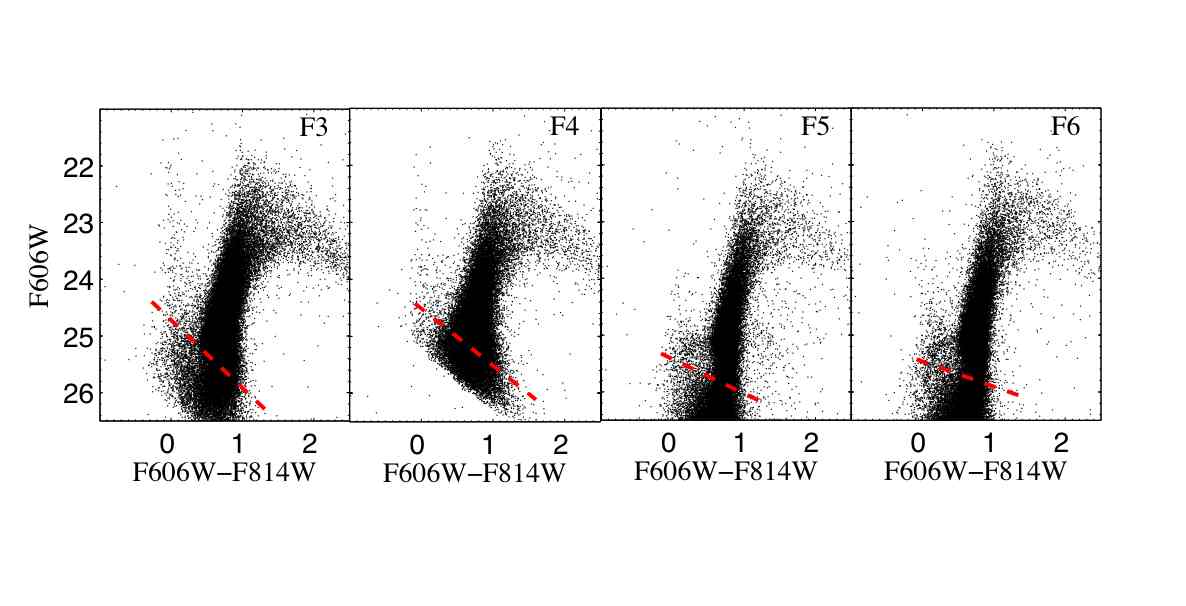
Figure 22.— CMDs of the fields analyzed to investigate the presence of a blue plume in M32. The magnitudes are calibrated onto the Vega mag WFPC2 system. The dashed red line indicates the 50% completeness level of the data. We can see a blue plume above the 50% completeness level in all fields. More information about these fields and CMDs can be found in Table 6.

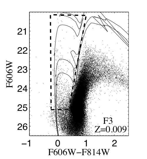
Figure 23.— CMD of F3 with young Padova isochrones (Marigo et al., 2008; Girardi et al., 2008) of ages 0.08, 0.2, and 0.3 Gyr for a metallicity of $Z=0.009$ superimposed. We have assumed a reddening of $E(B-V)=0.08$ (Burstein & Heiles, 1982) and a true distance modulus of $\mu_{0}=24.53$ (this paper). The dashed-box represents the region from which we counted blue plume stars in this field.

Thus, it remains as an open question as to why the BP in M32 was not seen in earlier optical data. The fact that the $B$ band has not been previously observed but just the $V$ and $I$ cannot be reason because the BP is clearly visible in the $VI$ archival observations shown in Figure 22 and in Alonso-García et al. (2004). The BP was not however seen in G96, who observed with the same WFPC2 camera. However, the G96 data are closer to the center of M32 than those of Alonso-García et al. It is likely that the extreme crowding affecting the region of interest made the detection of the blue plume impossible in previous works. In this context it is interesting to compare M32 with the dwarf elliptical (dE) NGC 205, also satellite of M31, which has been known to have blue OB-type stars since Baade (1951, see also and references therein). Only recently has there been a significant and genuine population of young blue stars observed in its center using ACS/HRC data (Monaco et al., 2009). Previous works of this galaxy have shown no BP stars, or some blue stars in the WFPC2 $VI$ data (see Butler & Martínez-Delgado, 2005) although, curiously, few. The fact that in NGC 205, a genuine BP was only observed with ACS/HRC data whereas it was not (significantly) seen in previous works, favors our hypothesis that the previous non-detection of a BP in M32 was a problem of crowding and resolution.

References

- Ajhar et al. (1996) Ajhar, E. A., Grillmair, C. J., Lauer, T. R., Baum, W. A., Faber, S. M., Holtzman, J. A., Lynds, C. R., & O’Neil, Jr., E. J. 1996, AJ, 111, 1110
- Alonso-García et al. (2004) Alonso-García, J., Mateo, M., & Worthey, G. 2004, AJ, 127, 868
- Alves et al. (2002) Alves, D. R., Rejkuba, M., Minniti, D., & Cook, K. H. 2002, ApJ, 573, L51
- Alves & Sarajedini (1999) Alves, D. R., & Sarajedini, A. 1999, ApJ, 511, 225
- Aparicio et al. (2001) Aparicio, A., Carrera, R., & Martínez-Delgado, D. 2001, AJ, 122, 2524
- Aparicio & Gallart (2004) Aparicio, A., & Gallart, C. 2004, AJ, 128, 1465
- Arp (1966) Arp, H. 1966, ApJS, 14, 1
- Baade (1951) Baade, W. 1951, Publications of Michigan Observatory, 10
- Barker et al. (2007) Barker, M. K., Sarajedini, A., Geisler, D., Harding, P., & Schommer, R. 2007, AJ, 133, 1138
- Bekki et al. (2001) Bekki, K., Couch, W. J., Drinkwater, M. J., & Gregg, M. D. 2001, ApJ, 557, L39
- Bender et al. (1992) Bender, R., Burstein, D., & Faber, S. M. 1992, ApJ, 399, 462
- Bica et al. (1990) Bica, E., Alloin, D., & Schmidt, A. A. 1990, A&A, 228, 23
- Brown et al. (2000) Brown, T. M., Bowers, C. W., Kimble, R. A., Sweigart, A. V., & Ferguson, H. C. 2000, ApJ, 532, 308
- Brown et al. (2004) Brown, T. M., Ferguson, H. C., Smith, E., Kimble, R. A., Sweigart, A. V., Renzini, A., & Rich, R. M. 2004, AJ, 127, 2738
- Brown et al. (2006) Brown, T. M., Smith, E., Ferguson, H. C., Rich, R. M., Guhathakurta, P., Renzini, A., Sweigart, A. V., & Kimble, R. A. 2006, ApJ, 652, 323
- Brown et al. (2008) Brown, T. M., Smith, E., Ferguson, H. C., Sweigart, A. V., Kimble, R. A., & Bowers, C. W. 2008, ApJ, 682, 319
- Burstein et al. (1984) Burstein, D., Faber, S. M., Gaskell, C. M., & Krumm, N. 1984, ApJ, 287, 586
- Burstein & Heiles (1982) Burstein, D., & Heiles, C. 1982, AJ, 87, 1165
- Butler & Martínez-Delgado (2005) Butler, D. J., & Martínez-Delgado, D. 2005, AJ, 129, 2217
- Cappellari et al. (2006) Cappellari, M., et al. 2006, MNRAS, 366, 1126
- Caputo et al. (1989) Caputo, F., Chieffi, A., Tornambe, A., Castellani, V., & Pulone, L. 1989, ApJ, 340, 241
- Carrera et al. (2002) Carrera, R., Aparicio, A., Martínez-Delgado, D., & Alonso-García, J. 2002, AJ, 123, 3199
- Cassisi et al. (2001) Cassisi, S., Castellani, V., Degl’Innocenti, S., Piotto, G., & Salaris, M. 2001, A&A, 366, 578
- Chiaberge et al. (2009) Chiaberge, M., Lim, P. L., Kozhurina-Platais, V., Sirianni, M., & Mack, J. 2009, Updated CTE photometric correction for WFC and HRC, Tech. rep.
- Chilingarian et al. (2009) Chilingarian, I., Cayatte, V., Revaz, Y., Dodonov, S., Durand, D., Durret, F., Micol, A., & Slezak, E. 2009, Science, 326, 1379
- Choi et al. (2002) Choi, P. I., Guhathakurta, P., & Johnston, K. V. 2002, AJ, 124, 310
- Coelho et al. (2009) Coelho, P., Mendes de Oliveira, C., & Cid Fernandes, R. 2009, MNRAS, 396, 624
- Cole (1998) Cole, A. A. 1998, ApJ, 500, L137+
- Cole & The Lcid Team (2007) Cole, A. A., & The Lcid Team. 2007, in IAU Symposium, Vol. 241, IAU Symposium, ed. A. Vazdekis & R. F. Peletier, 295–299
- Cowie et al. (1996) Cowie, L. L., Songaila, A., Hu, E. M., & Cohen, J. G. 1996, AJ, 112, 839
- Davidge (1991) Davidge, T. J. 1991, AJ, 102, 896
- Davidge & Jensen (2007) Davidge, T. J., & Jensen, J. B. 2007, AJ, 133, 576
- de Freitas Pacheco & Barbuy (1995) de Freitas Pacheco, J. A., & Barbuy, B. 1995, A&A, 302, 718
- de Marchi et al. (2006) de Marchi, F., de Angeli, F., Piotto, G., Carraro, G., & Davies, M. B. 2006, A&A, 459, 489
- Dolphin (2000) Dolphin, A. E. 2000, PASP, 112, 1383
- Elston & Silva (1992) Elston, R., & Silva, D. R. 1992, AJ, 104, 1360
- Faber (1973) Faber, S. M. 1973, ApJ, 179, 423
- Faber & Jackson (1976) Faber, S. M., & Jackson, R. E. 1976, ApJ, 204, 668
- Ferguson & Johnson (2001) Ferguson, A. M. N., & Johnson, R. A. 2001, ApJ, 559, L13
- Ferraro et al. (2004) Ferraro, F. R., Beccari, G., Rood, R. T., Bellazzini, M., Sills, A., & Sabbi, E. 2004, ApJ, 603, 127
- Ferraro et al. (1999) Ferraro, F. R., Messineo, M., Fusi Pecci, F., de Palo, M. A., Straniero, O., Chieffi, A., & Limongi, M. 1999, AJ, 118, 1738
- Fiorentino et al. (2010) Fiorentino, G., et al. 2010, ApJ, 708, 817
- Fontanot et al. (2009) Fontanot, F., De Lucia, G., Monaco, P., Somerville, R. S., & Santini, P. 2009, MNRAS, 397, 1776
- Ford et al. (1978) Ford, H. C., Jacoby, G. H., & Jenner, D. C. 1978, ApJ, 223, 94
- Freedman (1992a) Freedman, W. L. 1992a, AJ, 104, 1349
- Freedman (1992b) Freedman, W. L. 1992b, in IAU Symposium, Vol. 149, The Stellar Populations of Galaxies, ed. B. Barbuy & A. Renzini, 169–+
- Freedman & Madore (1990) Freedman, W. L., & Madore, B. F. 1990, ApJ, 365, 186
- Fuentes-Carrera et al. (2008) Fuentes-Carrera, I., Jablonka, P., Sarajedini, A., Bridges, T., Djorgovski, G., & Meylan, G. 2008, A&A, 483, 769
- Fusi Pecci et al. (1990) Fusi Pecci, F., Ferraro, F. R., Crocker, D. A., Rood, R. T., & Buonanno, R. 1990, A&A, 238, 95
- Gallart (1998) Gallart, C. 1998, ApJ, 495, L43+
- Gallart et al. (1996) Gallart, C., Aparicio, A., & Vilchez, J. M. 1996, AJ, 112, 1928
- Gallart et al. (2005) Gallart, C., Zoccali, M., & Aparicio, A. 2005, ARA&A, 43, 387
- Gallazzi et al. (2008) Gallazzi, A., Brinchmann, J., Charlot, S., & White, S. D. M. 2008, MNRAS, 383, 1439
- Gallazzi et al. (2005) Gallazzi, A., Charlot, S., Brinchmann, J., White, S. D. M., & Tremonti, C. A. 2005, MNRAS, 362, 41
- Girardi et al. (2002) Girardi, L., Bertelli, G., Bressan, A., Chiosi, C., Groenewegen, M. A. T., Marigo, P., Salasnich, B., & Weiss, A. 2002, A&A, 391, 195
- Girardi et al. (2000) Girardi, L., Bressan, A., Bertelli, G., & Chiosi, C. 2000, A&AS, 141, 371
- Girardi et al. (1998) Girardi, L., Groenewegen, M. A. T., Weiss, A., & Salaris, M. 1998, MNRAS, 301, 149
- Girardi & Salaris (2001) Girardi, L., & Salaris, M. 2001, MNRAS, 323, 109
- Girardi et al. (2008) Girardi, L., et al. 2008, PASP, 120, 583
- González (1993) González, J. J. 1993, PhD thesis, Thesis (PH.D.)–UNIVERSITY OF CALIFORNIA, SANTA CRUZ, 1993.Source: Dissertation Abstracts International, Volume: 54-05, Section: B, page: 2551.
- Graham (2002) Graham, A. W. 2002, ApJ, 568, L13
- Gregg et al. (2004) Gregg, M. D., Ferguson, H. C., Minniti, D., Tanvir, N., & Catchpole, R. 2004, AJ, 127, 1441
- Grillmair et al. (1996a) Grillmair, C. J., Ajhar, E. A., Faber, S. M., Baum, W. A., Holtzman, J. A., Lauer, T. R., Lynds, C. R., & O’Neil, Jr., E. J. 1996a, AJ, 111, 2293
- Grillmair et al. (1996b) Grillmair, C. J., et al. 1996b, AJ, 112, 1975
- Harris et al. (1999) Harris, G. L. H., Harris, W. E., & Poole, G. B. 1999, AJ, 117, 855
- Hodge (1973) Hodge, P. W. 1973, ApJ, 182, 671
- Holtzman et al. (2006) Holtzman, J. A., Afonso, C., & Dolphin, A. 2006, ApJS, 166, 534
- Holtzman et al. (1995) Holtzman, J. A., Burrows, C. J., Casertano, S., Hester, J. J., Trauger, J. T., Watson, A. M., & Worthey, G. 1995, PASP, 107, 1065
- Holtzman et al. (1991) Holtzman, J. A., et al. 1991, ApJ, 369, L35
- Hopkins & Beacom (2006) Hopkins, A. M., & Beacom, J. F. 2006, ApJ, 651, 142
- Hurley-Keller et al. (1999) Hurley-Keller, D., Mateo, M., & Grebel, E. K. 1999, ApJ, 523, L25
- Iben (1968) Iben, Jr., I. 1968, Nature, 220, 143
- Jensen et al. (2003) Jensen, J. B., Tonry, J. L., Barris, B. J., Thompson, R. I., Liu, M. C., Rieke, M. J., Ajhar, E. A., & Blakeslee, J. P. 2003, ApJ, 583, 712
- King et al. (1985) King, C. R., Da Costa, G. S., & Demarque, P. 1985, ApJ, 299, 674
- Komatsu et al. (2010) Komatsu, E., et al. 2010, ArXiv e-prints
- Kormendy (1985) Kormendy, J. 1985, ApJ, 295, 73
- Kormendy et al. (2009) Kormendy, J., Fisher, D. B., Cornell, M. E., & Bender, R. 2009, ApJS, 182, 216
- Lauer (1999) Lauer, T. R. 1999, PASP, 111, 227
- Lauer et al. (1998) Lauer, T. R., Faber, S. M., Ajhar, E. A., Grillmair, C. J., & Scowen, P. A. 1998, AJ, 116, 2263
- Lee et al. (1993) Lee, M. G., Freedman, W. L., & Madore, B. F. 1993, ApJ, 417, 553
- Lucy (1974) Lucy, L. B. 1974, AJ, 79, 745
- Mapelli et al. (2009) Mapelli, M., Ripamonti, E., Battaglia, G., Tolstoy, E., Irwin, M. J., Moore, B., & Sigurdsson, S. 2009, MNRAS, 396, 1771
- Mapelli et al. (2004) Mapelli, M., Sigurdsson, S., Colpi, M., Ferraro, F. R., Possenti, A., Rood, R. T., Sills, A., & Beccari, G. 2004, ApJ, 605, L29
- Mapelli et al. (2006) Mapelli, M., Sigurdsson, S., Ferraro, F. R., Colpi, M., Possenti, A., & Lanzoni, B. 2006, MNRAS, 373, 361
- Maraston & Thomas (2000) Maraston, C., & Thomas, D. 2000, ApJ, 541, 126
- Marigo et al. (2008) Marigo, P., Girardi, L., Bressan, A., Groenewegen, M. A. T., Silva, L., & Granato, G. L. 2008, A&A, 482, 883
- Mateo et al. (1995) Mateo, M., Fischer, P., & Krzeminski, W. 1995, AJ, 110, 2166
- McConnachie et al. (2005) McConnachie, A. W., Irwin, M. J., Ferguson, A. M. N., Ibata, R. A., Lewis, G. F., & Tanvir, N. 2005, MNRAS, 356, 979
- Momany et al. (2007) Momany, Y., Held, E. V., Saviane, I., Zaggia, S., Rizzi, L., & Gullieuszik, M. 2007, A&A, 468, 973
- Monaco et al. (2009) Monaco, L., Saviane, I., Perina, S., Bellazzini, M., Buzzoni, A., Federici, L., Fusi Pecci, F., & Galleti, S. 2009, A&A, 502, L9
- Nieto & Prugniel (1987) Nieto, J., & Prugniel, P. 1987, A&A, 186, 30
- Noeske et al. (2007) Noeske, K. G., et al. 2007, ApJ, 660, L47
- O’Connell (1980) O’Connell, R. W. 1980, ApJ, 236, 430
- Olsen et al. (2006) Olsen, K. A. G., Blum, R. D., Stephens, A. W., Davidge, T. J., Massey, P., Strom, S. E., & Rigaut, F. 2006, AJ, 132, 271
- Origlia & Leitherer (2000) Origlia, L., & Leitherer, C. 2000, AJ, 119, 2018
- Ortolani et al. (1992) Ortolani, S., Bica, E., & Barbuy, B. 1992, A&AS, 92, 441
- Paczynski & Stanek (1998) Paczynski, B., & Stanek, K. Z. 1998, ApJ, 494, L219+
- Percival & Salaris (2003) Percival, S. M., & Salaris, M. 2003, MNRAS, 343, 539
- Perryman & ESA (1997) Perryman, M. A. C., & ESA, eds. 1997, ESA Special Publication, Vol. 1200, The HIPPARCOS and TYCHO catalogues. Astrometric and photometric star catalogues derived from the ESA HIPPARCOS Space Astrometry Mission
- Perryman et al. (1997) Perryman, M. A. C., et al. 1997, A&A, 323, L49
- Pickles (1985) Pickles, A. J. 1985, ApJ, 296, 340
- Piotto et al. (2004) Piotto, G., et al. 2004, ApJ, 604, L109
- Rejkuba et al. (2005) Rejkuba, M., Greggio, L., Harris, W. E., Harris, G. L. H., & Peng, E. W. 2005, ApJ, 631, 262
- Renzini & Buzzoni (1986) Renzini, A., & Buzzoni, A. 1986, in Astrophysics and Space Science Library, Vol. 122, Spectral Evolution of Galaxies, ed. C. Chiosi & A. Renzini, 195–231
- Renzini & Fusi Pecci (1988) Renzini, A., & Fusi Pecci, F. 1988, ARA&A, 26, 199
- Richardson (1972) Richardson, W. H. 1972, Journal of the Optical Society of America (1917-1983), 62, 55
- Robin et al. (2003) Robin, A. C., Reylé, C., Derrière, S., & Picaud, S. 2003, A&A, 409, 523
- Rood (1972) Rood, R. T. 1972, ApJ, 177, 681
- Rose (1985) Rose, J. A. 1985, AJ, 90, 1927
- Rose (1994) —. 1994, AJ, 107, 206
- Rose et al. (2005) Rose, J. A., Arimoto, N., Caldwell, N., Schiavon, R. P., Vazdekis, A., & Yamada, Y. 2005, AJ, 129, 712
- Saha et al. (2006) Saha, A., Thim, F., Tammann, G. A., Reindl, B., & Sandage, A. 2006, ApJS, 165, 108
- Sakai et al. (1997) Sakai, S., Madore, B. F., Freedman, W. L., Lauer, T. R., Ajhar, E. A., & Baum, W. A. 1997, ApJ, 478, 49
- Santini et al. (2009) Santini, P., et al. 2009, A&A, 504, 751
- Sarajedini & Forrester (1995) Sarajedini, A., & Forrester, W. L. 1995, AJ, 109, 1112
- Sarajedini et al. (2009) Sarajedini, A., Mancone, C. L., Lauer, T. R., Dressler, A., Freedman, W., Trager, S. C., Grillmair, C., & Mighell, K. J. 2009, AJ, 138, 184
- Schechter & Dressler (1987) Schechter, P. L., & Dressler, A. 1987, AJ, 94, 563
- Schiavon et al. (2004) Schiavon, R. P., Caldwell, N., & Rose, J. A. 2004, AJ, 127, 1513
- Sirianni et al. (2005) Sirianni, M., et al. 2005, PASP, 117, 1049
- Stetson (1987) Stetson, P. B. 1987, PASP, 99, 191
- Stetson (1994) —. 1994, PASP, 106, 250
- Stetson & Harris (1988) Stetson, P. B., & Harris, W. E. 1988, AJ, 96, 909
- Sweigart (1987) Sweigart, A. V. 1987, ApJS, 65, 95
- Sweigart & Gross (1978) Sweigart, A. V., & Gross, P. G. 1978, ApJS, 36, 405
- Tonry et al. (2001) Tonry, J. L., Dressler, A., Blakeslee, J. P., Ajhar, E. A., Fletcher, A. B., Luppino, G. A., Metzger, M. R., & Moore, C. B. 2001, ApJ, 546, 681
- Trager et al. (2000a) Trager, S. C., Faber, S. M., Worthey, G., & González, J. J. 2000a, AJ, 120, 165
- Trager et al. (2000b) —. 2000b, AJ, 119, 1645
- Trager et al. (2005) Trager, S. C., Worthey, G., Faber, S. M., & Dressler, A. 2005, MNRAS, 362, 2
- Tremonti et al. (2004) Tremonti, C. A., et al. 2004, ApJ, 613, 898
- Udalski (1998) Udalski, A. 1998, Acta Astronomica, 48, 383
- Williams (2002) Williams, B. F. 2002, MNRAS, 331, 293
- Worthey (1994) Worthey, G. 1994, ApJS, 95, 107
- Worthey (1998) —. 1998, PASP, 110, 888
- Worthey (2004) —. 2004, AJ, 128, 2826
- Worthey et al. (1996) Worthey, G., Dorman, B., & Jones, L. A. 1996, AJ, 112, 948
- Worthey et al. (2005) Worthey, G., España, A., MacArthur, L. A., & Courteau, S. 2005, ApJ, 631, 820
- Worthey et al. (2004) Worthey, G., Mateo, M., Alonso-García, J., & España, A. L. 2004, PASP, 116, 295
- Xu & Li (2004) Xu, H. Y., & Li, Y. 2004, A&A, 418, 225
- Ziegler & Bender (1998) Ziegler, B. L., & Bender, R. 1998, A&A, 330, 819
- Zoccali et al. (2003) Zoccali, M., et al. 2003, A&A, 399, 931