Detectability of ultrahigh energy cosmic ray signatures
in gamma rays

The injection of ultra-high energy cosmic rays in the intergalactic medium leads to the production of a GeV-TeV gamma-ray halo centered on the source location, through the production of a high electromagnetic component in the interactions of the primary particles with the radiation backgrounds. This paper examines the prospects for the detectability of such gamma ray halos. We explore a broad range of astrophysical parameters, including the inhomogeneous distribution of magnetic fields in the large scale structure as well as various possible chemical compositions and injection spectra; and we consider the case of a source located outside clusters of galaxies. With respect to the gamma-ray flux associated to synchrotron radiation of ultra-high energy secondary pairs, we demonstrate that it does not depend strongly on these parameters and conclude that its magnitude ultimately depends on the energy injected in the primary cosmic rays. Bounding the cosmic ray luminosity with the contribution to the measured cosmic ray spectrum, we then find that the gamma-ray halo produced by equal luminosity sources is well below current or planned instrument sensitivities. Only rare and powerful steady sources, located at distances larger than several hundreds of Mpc and contributing to a fraction $\gtrsim 10\,$% of the flux at $10^{19}\,$eV might be detectable. We also discuss the gamma-ray halos that are produced by inverse Compton/pair production cascades seeded by ultra-high energy cosmic rays. This latter signal strongly depends on the configuration of the extragalactic magnetic fields; it is dominated by the synchrotron signal on a degree scale if the filling factor of magnetic fields with $B\gtrsim 10^{-14}$ G is smaller than a few percents. Finally, we discuss briefly the case of nearby potential sources such as Centaurus A.

1 Introduction

The quest for the sources of ultrahigh energy cosmic rays has long been associated with the search of their secondary radiative signatures. While propagating, the former indeed produce very high energy photons through the interactions with the ambient backgrounds; and gamma rays should be valuable tools for the identification of the birthplace of the primary cosmic rays as they travel in a straight manner, contrarily to charged particles.

The detection of such photon fluxes is far from straightforward, however. On purely astrophysical grounds, the propagation of gamma rays with energy exceeding several TeV is obstructed by their relatively short pathlength of interaction with cosmic microwave background (CMB) and infrared photons. These interactions lead to the production of high energy electron and positron pairs which in turn up-scatter CMB or radio photons by inverse Compton processes, initiating electromagnetic cascades. One does not expect to observe gamma rays of energy above $\sim 100$ TeV from sources located beyond a horizon of a few megaparsecs (Gould & Schréder 1967; Wdowczyk et al. 1972; Protheroe 1986; Protheroe & Stanev 1993). Below this energy, the detection of the gamma ray signal originating from ultrahigh energy cosmic rays depends on the luminosity and angular extension of the observed object and obviously on the sensitivity and angular resolution of the available instruments.

Intergalactic magnetic fields inevitably come into play in this picture: i) primary cosmic rays can be deflected by the magnetic field surrounding the source prior to the production of secondary photons/electrons/positrons, ii) secondary electrons and positrons produced by cosmic ray interactions or by photon-photon interactions can also be deflected by the intergalactic magnetic field during the cascade. In both cases the ultimate gamma ray emission can experience a sizable spread around the ultrahigh energy cosmic ray source.

Aharonian (2002) and Gabici & Aharonian (2005) have observed that the magnetic field environment of the source may also lead to the generation of a multi-GeV gamma ray halo around ultra-high energy cosmic ray sources. The idea is the following: for high enough energies and in the presence of a magnetic field large enough in the surroundings of the source, the electron and positron pairs produced through the interaction of ultra-high energy particles with the ambient backgrounds may lose a significant fraction of their energy through synchrotron emission. This synchrotron component falls around $\sim 10$ GeV, below the pair creation threshold, hence it will not be affected by further electromagnetic cascading. Assuming that the source is located at 100 Mpc distance, at the center of a homogeneously magnetized sphere of radius 20 Mpc with $B=1\leavevmode\nobreak\$nG, Gabici & Aharonian (2005) estimate that this signal would have an angular size of a fraction of degree (see also Aharonian et al. 2010). It could therefore appear point-like for instruments such as the Fermi Space Telescope but as an extended source for future imaging Cerenkov telescopes.

This process is particularly interesting, because its signature could easily be differentiated from a point-like gamma ray signal emitted by leptonic or hadronic channels inside the source, associated with the acceleration of particles to energies possibly well below $10^{19}\,$eV. The dominant background to this synchrotron halo is actually the halo produced by multi-TeV electrons that undergo inverse Compton on the cosmic microwave background and that were seeded by multi-TeV photons at $\gtrsim\,$Mpc distance from the source (Aharonian et al. 1994). However, as discussed in the present paper, discrimination between these two signals should be possible thanks to the different dependencies of the angular images on physical parameters and on energy. Then, one could argue that the detection of a synchrotron halo around a powerful source would constitute an unambiguous signature of acceleration to ultra-high energies in this source: first of all, the inverse Compton cooling length of electrons with energy $1\,{\rm TeV}\,\lesssim\,E_{e}\lesssim 10^{17}\,$eV is smaller than $300\,$kpc, hence the gamma-ray signal of very high energy electrons produced in the source would appear point-like at distances $\gtrsim 100\,$Mpc; furthermore, secondary electrons generally carry a few percents of the parent proton energy, so that $\gtrsim 10^{17}\,$eV secondary electrons correspond to $\gtrsim 10^{19}\,$eV protons; finally, if the radiating electrons are seeded away from the source by high energy nuclei, these nuclei must carry an energy $\gtrsim 10^{19}\,$eV as lower energy nuclei are essentially immune to radiative losses.

Given our state of knowledge on the sources of ultrahigh energy cosmic rays, the detection of such a halo would have a lasting impact on this field of research. The detectability of such signals thus deserves close scrutiny.

The production of gamma ray signatures of ultrahigh energy cosmic rays have been studied numerically by Ferrigno et al. (2004) and Armengaud et al. (2006). However, the former authors have focused their study on the Compton cascades following the production of ultrahigh energy photons and pairs close to the source and they have neglected the deflection imparted by the surrounding magnetic fields which dilutes the gamma-ray signal (Gabici & Aharonian 2005), while Armengaud et al. (2006) have addressed both the synchrotron emission of secondary pairs and the Compton cascading down to TeV energies, albeit for the particular case of a source located in a magnetized cluster of galaxies. The high magnetic field that prevails in such environments increases the residence time of primary and secondary charged particles and thus also increases the gamma ray flux.

The present paper aims at examining the prospects for the detectability of gamma ray halos around ultrahigh energy cosmic ray sources, relaxing most of the assumptions made in the above previous studies. In particular, we discuss the more general case of a source located in the field, outside clusters of galaxies. We focus our discussion on the synchrotron signal emitted by secondary pairs, which offers a possibility of unambiguous detection; nevertheless, the deflection and the dilution of the Compton cascading gamma ray signal at TeV energies is also discussed. Going further than Aharonian (2002) and Gabici & Aharonian (2005), we take into account the inhomogeneous distribution of the magnetic fields in the source environment. We also relax the assumption of a pure proton composition of ultra high energy cosmic rays, underlying to the above studies. The chemical composition of ultrahigh energy cosmic rays indeed remains an open question. While experiments such as the Fly’s Eye and HiRes have suggested a transition from heavy to light above $\sim 10^{18.5}$ eV (Bird et al. 1993; Abbasi et al. 2005, 2010), the most recent measurements made with the Pierre Auger Observatory rather point towards a heavy composition above $10^{19}\,$eV (Unger et al. 2007; Abraham et al. 2009, 2010). As the energy losses and magnetic deflection of high energy nuclei differ from those of a proton of a same energy, one should naturally expect different gamma ray signatures.

The lay-out of the present paper is as follows. In Section 2, we first test the dependence of the gamma ray flux produced by ultrahigh energy cosmic rays on the type, intensity and structure of magnetized environments. We also discuss the effects of various chemical compositions and injection spectra. We conclude on the robustness of the gamma ray signature according to these parameters and find that the normalization and thus the detectability of this flux ultimately depends on the energy injected in the primary cosmic rays. In Section 3, we discuss the detectability of ultrahigh energy cosmic ray signatures in gamma rays. Applying the results of our calculations, we show that the average type of sources contributing to the ultrahigh energy cosmic ray spectrum produces a gamma ray flux more than two orders of magnitudes lower than the sensitivity of the current and upcoming instruments. We then explore the case of rare powerful sources with cosmic ray luminosity over energy $10^{19}$ eV of $L_{19}>10^{44-46}$ erg s^-1. We assume throughout this paper that sources emit isotropically and discuss how the conclusions are modified for beamed emission in Section 4. The gamma ray signatures of those sources could be detectable provided that they are located far enough not to overshoot the observed cosmic ray spectrum. Finally, we also briefly discuss the detection of nearby sources, considering the radiogalaxy Centaurus A as a protoypical example. We draw our conclusions in Section 4.

2 Simulations

As mentioned above, we focus our discussion on the synchrotron signal that can be produced close to the source by very high energy electrons and positrons, that result themselves from the interactions of primary cosmic rays. The signal associated to inverse Compton cascades of these electrons/positrons on radiation backgrounds will be discussed in Section 3.3.

The secondary electrons and positrons are created through one of the three following channels: i) by the decay of a charged pion produced during a photo-hadronic interaction ($A\,\gamma\rightarrow\pi^{+}+...$, then $\pi^{+}\rightarrow\mu^{+}\,\nu_{\mu}$, and $\mu^{+}\rightarrow e^{+}\,\nu_{e}\,\bar{\nu_{\mu}}$, with $A$ a cosmic ray nucleus), ii) by photo pair production during an interaction with a background photon ($A\,\gamma\rightarrow e^{+}\,e^{-}+...$), or iii) by the disintegration of a neutral pion into ultrahigh energy photons which then interact with CMB and radio backgrounds to produce electron and positron pairs ($A\,\gamma\rightarrow\pi^{0}+...$, then $\pi^{0}\rightarrow 2\gamma$, and $\gamma\,\gamma_{\rm bg}\rightarrow e^{+}\,e^{-}$, with $\gamma_{\rm bg}$ a cosmic background photon). In all cases, the resulting electrons and positrons typically carry up to a few percents of the initial cosmic ray energy.

While propagating in the intergalactic medium, these ultrahigh energy electrons and positrons up-scatter CMB or radio photons through inverse Compton processes and/or they lose energy through synchrotron radiation. Following  Gabici & Aharonian (2005), the effective inverse Compton cooling length on the CMB and radio backgrounds can be written as $x_{e\gamma}\,\approx\,5\,{\rm Mpc}\,(E_{e}/10^{18}\,{\rm eV})^{\alpha_{\rm IC}}$, with $\alpha_{\rm IC}=1$ if the electron energy $E_{e}\lesssim 10^{18}\,$eV and $\alpha_{\rm IC}\simeq 0.25$ if $10^{18}\,{\rm eV}\,\lesssim E_{e}\lesssim 10^{20}\,$eV. Above $10^{18}$ eV, the scaling of the cooling length actually depends on the assumptions made for the radio background, which is unfortunately not very well known. The possible differences that such uncertainties could introduce should however not affect the results discussed in this paper. This length scale has to be compared with the synchrotron cooling length

$$x_{eB}\sim 3.8\leavevmode\nobreak\ {\rm kpc}\,\left(\frac{B}{10\leavevmode\nobreak\ {\rm nG}}\right)^{-2}\left(\frac{E_{e}}{10^{19}\leavevmode\nobreak\ {\rm eV}}\right)^{-1}\ ,$$ (1)

where $B$ is the magnetic field intensity (assumed homogeneous over this distance) and $E_{e}$ the electron or positron energy.

As discussed in Gabici & Aharonian (2005), the opposite scalings of $x_{e\gamma}$ and $x_{eB}$ with electron energy imply the existence of a cross-over energy $E_{\times}$, which depends on $B$ and is such that beyond $E_{\times}$, electrons mainly cool via synchrotron instead of undergoing an inverse Compton cascade. For a magnetic field of intensity $B=10^{-9}B_{\rm nG}\,$G, $E_{\times}\sim 10^{18}\,{\rm eV}B_{\rm nG}^{-1}$ for $B_{\rm nG}\gtrsim 1$, $E_{\times}\sim 10^{18}\,{\rm eV}B_{\rm nG}^{-1.6}$ for $1\gtrsim\,B_{\rm nG}\gtrsim 0.1$ and $E_{\times}\sim 10^{20}\,{\rm eV}B_{\rm nG}^{-1}$ for $0.1\gtrsim\,B_{\rm nG}$, see Fig. 1 of Gabici & Aharonian (2005) and see Lee (1998) for further details on the cascade physics.

Finally, the emitted synchrotron photon spectrum peaks at the energy:

$$E_{\gamma,{\rm syn}}\sim 68\,{\rm GeV}\,\left(\frac{B}{10\leavevmode\nobreak\ {\rm nG}}\right)\left(\frac{E_{e}}{10^{19}\leavevmode\nobreak\ {\rm eV}}\right)^{2}\,.$$ (2)

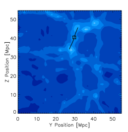
Figure 1: Distribution of the magnetic field intensity in the region surrounding an ultrahigh energy cosmic ray source. Each panel is a 1.1 Mpc thick (size of a grid cell) slice of the simulated Universe, cut along the axis perpendicular to the observed plan. From left to right, the distribution is of type “isotropic” (Eq. 3), “anisotropic” (Eq. 4) and “contrasted” (Eq. 5). The color code is the same for all the panels and the values indicated on the right hand side correspond to the logarithm of the magnetic field intensity in nano Gauss. The black line indicates the axis of the filament that is studied throughout this paper and the black square the chosen position of the source. The normalization factor equals $B_{0}=1$ nG.

2.1 Magnetic field configuration

Our current knowledge on the structure of magnetic fields at large scales is very poor. It mainly stems from the lack of observations due to the intrinsic weakness of the fields. Moreover, no satisfactory theory has been established to explain the origins of these fields and the further magnetic enrichment of the Universe. There is now a decade of history of numerical simulations that endeavor to model the distribution of the magnetic field at large scales. One may cite in particular the works of Ryu et al. (1998), Dolag et al. (2004, 2005), Sigl et al. (2004) and most recently Das et al. (2008). In these studies, magnetized seeds are injected in a cosmological simulation and the overall magnetic field then evolves coupled with the underlying baryonic matter. The final amplitude of the field is set to adjust the measured intensity inside clusters of galaxies (in Das et al. 2008 the amplitude is not arbitrary but is directly estimated from the gas kinetic property and corresponds nevertheless to the observations inside clusters). Unfortunately, these various simulations do not converge as to the present-day configuration of extragalactic magnetic fields (see for example Fig. 1 of Kotera & Lemoine 2008a) and consequently, they also diverge as to the effect of these magnetic fields on the transport of ultrahigh energy cosmic rays. The cause of this difference likely lies in the choice of initial data, which cannot be constrained with our current knowledge. Given the fact that such simulations are time consuming, these tools cannot be considered as practical.

In view of this situation, we explore the influence of three typical types of magnetic field structures on the gamma ray emission, following the method developed by Kotera & Lemoine (2008a). We map the magnetic field intensity distribution according to the underlying matter density $\rho$, assuming the relation $B=B_{0}\,f(\rho)$, where $B_{0}$ is a normalization factor, and the dimensionless function $f$ may be modelled as:

$$f_{\rm iso}(\rho) \,=\,\rho^{2/3}\ ,$$ (3)

$$f_{\rm ani}(\rho) \,=\,\rho^{0.9}\ ,$$ (4)

$$f_{\rm contrast}(\rho) \,=\,\rho\left[1+\left({\rho\over\langle\rho\rangle}\right)^{-2}\right]^{-1}.$$ (5)

Note that $B_{0}$ corresponds approximately to the mean value of the magnetic field in the Universe. These phenomenological relationships greatly simplify the numerical procedure to obtain a map of the extragalactic magnetic field since a pure dark matter (i.e. non hydrodynamical) simulation of large scale structure provides a sufficiently good description of the density field. These relationships are motivated by physical arguments related to the mechanism of amplification of magnetic fields during structure formation and they encapture the scalings observed in numerical simulations up to the uncertainty inherent in such simulations (see the corresponding discussion in Dolag 2006 and Kotera & Lemoine 2008a). The first relation is typically expected if baryonic matter undergoes an isotropic collapse. In dense regions of the Universe where viscosity and shear effects govern the evolution of the magnetized plasma however, the relation would get closer to Eq. (4). This formula can be derived analytically in the case of an anisotropic collapse along one or two dimensions, in filaments or sheets for example (King & Coles 2006). The last model is an ad-hoc modeling of the suppression of magnetic fields in the voids of large structure which leaves unchanged the distribution in the dense intergalactic medium (meaning $\rho>\langle\rho\rangle$). It thus allows to model a situation in which the magnetic enrichment of the intergalactic medium is related to structure formation, for instance through the pollution by starburst galaxies and/or radio-galaxies (see the corresponding discussion in Kotera & Lemoine 2008b). In the following, we will refer to these three models as “isotropic”, “anisotropic” and “contrasted” respectively.

In order to have a representative sample of the underlying matter density at large scales, we use a three-dimensional output (at redshift $z=0$) of a cosmological Dark Matter simulation provided by S. Colombi. It assumes a $\Lambda$CDM model with $\Omega_{\mathrm{m}}=0.3$, $\Omega_{\mathrm{\Lambda}}=0.7$ and Hubble constant $h\equiv H_{0}/(100$ km s^-1 Mpc${}^{-1})=0.7$. The simulation models a $200\,h^{-1}$ Mpc comoving periodic cube split in $256^{3}$ cells, where the Dark Matter overdensity is computed. We do not resolve structures below the Jeans length, which implies that we can identify the computed Dark Matter distribution to a gas distribution.

2.2 Numerical code

We compute the gamma ray signal through numerical Monte Carlo simulations, using the code presented in Kotera et al. (2009). In a first step, we propagate ultrahigh energy cosmic rays (protons and heavier nuclei) in one of the three-dimensional magnetic field models described above. The coherence length $\lambda_{B}$ of the magnetic field is assumed to be constant throughout space and is set to $100\,$ kpc. This certainly is somewhat ad-hoc but: the coherence scale enters the calculation in the deflection angle under the form $B\sqrt{\lambda_{B}}$, hence discussing various normalizations of the magnetic field strength, as we do further below, allows to encapture different possible values for $\lambda_{B}$; furthermore, $100\,$kpc seems a reasonable compromise between an upper limit of a few hundreds of kpc for $\lambda_{B}$ based on the turn-around time of largest eddies  (Waxman & Bahcall 1999) and the typical galactic scales $\sim\,10-30\,$kpc, see Kotera & Lemoine (2008a) for a detailed discussion. The generation of secondary photons and electrons and positrons through pion production is treated in a discrete manner, as in Allard et al. (2006) for nuclei projectiles with $A>1$ and with SOPHIA (Mücke et al. 1999) for proton and neutron cosmic rays. Electron and positron pair creation through photo-hadronic processes is implemented as in Armengaud et al. (2006). For each time step (chosen to be much larger than the typical mean free path of pair photo-production processes), we assume that an ensemble of electron and positron pairs are generated with energies distributed according to a power law, and maximum energy depending on the primary particle. The use of an improved pair spectrum as computed in Kelner & Aharonian (2008) would lower the gamma ray flux resulting from direct pair production by a factor of a few in the range $E_{\gamma}\lesssim 10\,$GeV, and leave unchanged the prediction at a higher energy (Armengaud, private communication). Furthermore, we will show in the following that direct pair production processes provide a sub-dominant contribution to the overall gamma ray flux in the range $E_{\gamma}\,\gtrsim\,0.1\,$GeV, hence the overall difference is expected to be even smaller.

We investigate in this paper the possible detection of photons in the GeV-TeV energy range. Equation (2) suggests that, unless the source is embedded in a particularly strong field, the major contribution in this range will come from electrons of energy $E_{e}\gtrsim 10^{18}$ eV. The flux will thus essentially result from cosmic rays of energy higher than $E\sim 10^{19}\leavevmode\nobreak\$eV. For this reason, we chose to inject cosmic rays at the source between $E_{\rm min}=10^{17}$ eV et $E_{\rm max}=10^{20.5}$ eV. We assume our source to be stationary with (isotropic) cosmic ray luminosity integrated over $E=10^{19}$ eV of $L_{E,19}=10^{42-46}\leavevmode\nobreak\$erg s^-1, and a spectral index of $\alpha=2.3$.

We take into account photo-hadronic interactions with CMB and infrared photons. The diffuse infrared background is modelled according to the studies of Stecker et al. (2006). We do not take into account redshift evolution, as its effect is negligible as compared to the uncertainties on our other parameters. We also neglect baryonic interactions in view of the negligible density in the source environment.

Once the secondary particles produced during the propagation have been computed, we calculate the synchrotron photon fluxes, taking into account the competition with inverse Compton scattering by Monte Carlo over steps of size 100 kpc. The mean effective electron loss length is calculated following Gabici & Aharonian (2005), using the radio background data of Clark et al. (1970). We assume that each electron emits a synchrotron photon spectrum ${\rm d}N_{\gamma}/{\rm d}E_{\gamma}\propto E_{\gamma}^{-2/3}$ with a sharp cut-off above $E_{\rm c}\sim(2/3)\,E_{\rm\gamma,syn}$, where $E_{\rm\gamma,syn}$ is given by Eq. (2).

Regarding the photons produced through the neutral pion channel, we draw the interaction positions with CMB and radio photons using the mean free paths computed by Lee (1998). We assume that one of the electron-positron pair inherits of the total energy of the parent photon.

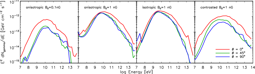
Figure 2: Flux of photons produced by synchrotron emission for a filament observed from the directions forming the indicated angles with its axis. The filament is located at 100 Mpc and harbors a source that injects a pure proton composition with (isotropic) luminosity of $L_{E,19}=10^{42}$ erg/s and a spectral index of 2.3. The four panels represent various models of magnetic fields. From left to right: “anisotropic” with $B_{0}=0.1\leavevmode\nobreak\$nG, “anisotropic” with $B_{0}=1\leavevmode\nobreak\$nG, “isotropic” with $B_{0}=1\leavevmode\nobreak\$nG and “contrasted” with $B_{0}=1\leavevmode\nobreak\$nG.

2.3 Synchrotron signal for various magnetic field configurations

We first study the influence of inhomogeneous magnetic fields on the gamma ray flux produced by ultrahigh energy cosmic rays near their source. In particular, we examine the case of a source placed in a rather dense region of a filament of large scale structure, see Fig. 1. On the transverse scale of the structure $l_{\perp}$, of order of a few Mpc, one expects the secondary electrons and positrons to be distributed isotropically around the source. A population of ultrahigh energy cosmic rays seeds the intergalactic medium with secondary pairs in a roughly homogeneous manner on the energy loss length scale of the interaction process $\lambda$, i.e. the number of electrons/positrons injected per unit time per unit distance to the source ${\rm d}N_{e}/{\rm d}r{\rm d}t$ does not depend on $r$ as long as $r\ll\lambda$. For ultrahigh energy protons, this length scale is $\sim 1\,$Gpc above $10^{19}\,$eV for pair production and $\sim 100\,$Mpc above $10^{20}\,$eV for pion production. From the point of view of secondary synchrotron $\gamma$ emission, however, the emission region is limited to the fraction of space in which the magnetic field is sufficiently intense for synchrotron cooling to predominate over inverse Compton cooling.

The bulk of gamma rays is produced by electrons of energy $E_{\rm e}\gtrsim 10^{19}\leavevmode\nobreak\$eV, themselves produced through pion production by protons of $E_{\rm p}\gtrsim 10^{20}\leavevmode\nobreak\$eV. In the absence of significant deflection experienced by these primary particles, one expects the synchrotron emission to be enhanced along the filament axis, where the magnetic field keeps a high value over a longer length than along the perpendicular direction (see Fig. 1). The whole structure where $x_{eB}<x_{e\gamma}$, i.e. $B_{\rm IGM}\gtrsim 0.5\,\mbox{nG}\,(E_{e}/10^{19}\,{\rm eV})^{-3/4}$ is then illuminated in synchrotron from electrons and positrons provided $x_{eB}<ct_{\rm esc}$, where $t_{\rm esc}$ denotes the escape timescale from the magnetized region. For a magnetic field with $B\sim 10\,$nG and coherence length $\lambda_{B}\lesssim 100\,$kpc, the Larmor time $t_{\rm L}\,\sim\,1\,{\rm Mpc}\,(E_{e}/10^{19}\,{\rm eV})(B/10\,{\rm nG})^{-1}\,\sim\lambda_{B}$, hence confinement is marginal and the escape length $t_{\rm esc}\sim l_{\perp}\gg x_{eB}$ (see Casse et al. 2002 for more details on the escape length).

At a given energy $E_{e}$, the ratio between the fluxes along and perpendicular to the filament should be of order $a/b$, where $a$ and $b$ are the characteristic lengths of the axis of the filament where $B_{\rm IGM}\gtrsim 0.5\,\mbox{nG}\,E_{e,19}^{-3/4}$.

Figure 2 depicts indeed such an effect. It represents the synchrotron emission produced by a filament at a distance of 100 Mpc, embedding a source of luminosity $L_{E,19}=10^{42}$ erg s^-1 and an injection spectral index of 2.3. One can notice that the difference between the highest and lowest flux values is of a factor $\sim 2-5$, which corresponds to the ratio between the filament major axis. For a narrower or longer filament, this interval would be more pronounced – which does not necessarily mean that the flux would be enhanced along the filament axis.

This difference of flux according to the observation angle disappears at low energy for the second and third panels of Fig. 2. This is intricately related to the combined effect of the configuration of the magnetic field and the ratio of electrons producing the observed peak of gamma rays. It corresponds to a coincidence and should not be viewed as an effect of diffusion of primary protons. We tested indeed that these differences remain present when cosmic rays are forced to propagate rectilinearly. For the contrasted magnetic field, the gamma-ray fluxes are overall lower, as the field strength diminishes sharply outside of the central part of the filament. The orthogonal section of the filament is thus substantially magnetized only over a short length, which consequently reduces the gamma-ray flux observed from $90^{\circ}$. For the isotropic and anisotropic cases with $B_{0}=1\leavevmode\nobreak\$nG, electrons and positrons experience a weaker field on average when they cross the filament orthogonally, instead of traveling through their entire length. For the flux observed at $90^{\circ}$, photons with energy $<10\leavevmode\nobreak\$GeV are thus generated by electrons of slightly higher energy ($E_{90}$) than in the $0^{\circ}$ case ($E_{0}$). By coincidence, $E_{90}$ corresponds approximately to the peak of distribution of secondary electrons, whereas $E_{0}$ is shifted according to the peak. The flux observed at $90^{\circ}$ is thus amplified for energies $<10$ GeV due to the enhanced number of electrons contributing to the emission, which brings up the fluxes at various observation angles closer. Finally, for the anisotropic case with $B_{0}=0.1$ nG, the emission is suppressed when the filament is not observed along its major axis, because of the weak mean field that particles experience (the mean field remains reasonably strong along the axis). The gap between the flux at $0^{\circ}$ and the other cases stems from this effect.

Most of all, Fig. 2 demonstrates that the photon flux around $E_{\gamma}\sim 10\leavevmode\nobreak\$GeV is fairly robust with respect to the various magnetic field configurations, which can be understood from Fig. 1: the extent of the magnetized region above $B\sim 1\leavevmode\nobreak\$nG is indeed not fundamentally modified by the chosen distribution and the photon flux is hardly more sensitive to the overall intensity of the field (in particular, we tested that a value of $B_{0}=10$ nG does not affect the results of more than a factor 2, for all magnetic configurations). All in all, for a quite reasonable normalization of the magnetic field, meaning an average $B_{0}\sim 0.1-10\,$nG at density contrast unity, and for various scalings of the magnetic field with density profile, the variations in flux remain smaller than an order of magnitude in the range $E_{\gamma}\sim 10-1000\,$GeV.

Figure 2 also illustrates that the energy at which the signal peaks depends only weakly on the normalization of the magnetic field $B_{0}$, and this remains true up to a few nano-Gauss. This can be understood qualitatively, assuming for simplicity the field to be homogeneous over the area of interest, with strength $B_{0}$. For $B_{0}=1\,$nG, the electron cross-over energy $E_{\times}$ beyond which electrons radiate in synchrotron reads $E_{\times}\simeq 10^{18}\,$eV (see the discussion in Sec. 2). However, the energy spectrum $E_{e}{\rm d}N_{e}/{\rm d}E_{e}$ of secondary electrons deposited in the source vicinity peaks at $\sim 10^{19}\,$eV, as a result of the competition between the opposite scalings with energy of the abundance of parent protons and of the parent proton energy loss rate. Therefore, the synchrotron signal is expected to peak at $E_{\gamma}\sim 10\,{\rm GeV}$, see Eq. 2 with $B_{0}=1\,$nG and $E_{e}=10^{19}\,$eV. Now, for $B_{0}=0.1\,$nG, the cross-over energy $E_{\times}\simeq 4\times 10^{19}\,$eV so that one should use $E_{e}=4\times 10^{19}\,$eV in Eq. 2 with $B_{0}=0.1\,$nG, giving $E_{\gamma}\sim 10\,$GeV again: the larger typical electron energy (among those radiating in synchrotron) compensates for the smaller value of $B_{0}$. As $B_{0}$ is increased significantly above $1\,$nG, the peak location of the gamma-ray signal will increase in proportion, as most of the secondary electron flux can be radiated in synchrotron.

Note that the flux should be cut off above $E_{\gamma}\sim 10$ TeV due to the opacity of the Universe to photons above this energy. This effect is not represented in these plots for simplicity, as its precise spectral shape depends on the distance $d$ to the source (while the sub-TeV gamma ray flux scales in proportion to $L_{\rm cr}/d^{2}$).

At lower energy ($E_{\gamma}\lesssim 1$ GeV), the flux intensity can vary by more than two orders of magnitude depending on the chosen magnetic configuration. In the low energy range, magnetic confinement indeed starts to play an important role. Furthermore, the inverse Compton energy loss length shortens drastically at these energies so that only strong magnetic fields can help avoiding the formation of an electromagnetic cascade and lead instead to synchrotron emission in the filament.

2.4 Synchrotron signal for various chemical compositions and injection spectra

In this section, we discuss the effect of the injected chemical composition and of the spectral index at the source. As discussed above, there are conflicting claims as to the measured chemical composition at ultrahigh energies; in particular, the HiRes experiment reports a light composition (Abbasi et al. 2010) while the Pierre Auger Observatory measurements point toward a composition that becomes increasingly heavier at energies above the ankle (Abraham et al. 2010). Theory is here of little help, as the source of ultrahigh energy cosmic rays is unknown; protons are usually considered as prime candidates because of their large cosmic abundance, but at the same time one may argue that a large atomic number facilitates acceleration to high energy.

In this framework, Lemoine & Waxman (2009) have proposed a test of the chemical composition of ultra-high energy cosmic rays on the sky, using the anisotropy patterns measured at various energies, instead of relying on measurements of the depth of maximum shower development. It is shown in particular that, at equal magnetic rigidities $E/Z$, one should observe a comparable or stronger anisotropy signal from the proton component than from the heavy nuclei component emitted by the source, even if the source injects protons and heavy nuclei in equal numbers at a given energy. When compared to the 99% c.l. anisotropy signal reported by the Pierre Auger Observatory at energies above $5.7\times 10^{19}\,$eV (Abraham et al. 2007, 2008a), one concludes that: if the composition is heavy at these energies, and if the source injects protons in at least equal number (at a given energy) as heavy nuclei, then one should observe a comparable or stronger anisotropy pattern above $5.7\times 10^{19}/Z\,$eV.

Future data will hopefully cast light on this issue, but in the meantime it is necessary to consider a large set of possible chemical compositions. We thus consider the following injection spectra:

1. Two pure proton compositions with indices $\alpha=2.3$ and 2.7. A soft spectral index of $\sim 2.7$ seems to be favored to fit the observed cosmic ray spectrum in the case of a pure proton composition, especially in the “dip-model” proposed by Berezinsky et al. (2006), where the transition between the Galactic and extragalactic components happens at relatively low energy ($E\sim 10^{17.5}$ eV).

2. A proton dominated mix composition with spectral index $\alpha=2.3$, based on Galactic cosmic ray abundances as in Allard et al. (2006). Such a spectrum is mostly proton dominated at ultra-high energies.

3. A pure iron composition with spectral index $\alpha=2.3$.

4. A mixed composition that was proposed by Allard et al. (2008), that contains 30% of iron. In this injection, the maximum proton energy is $E_{{\rm max},p}=10^{19}\leavevmode\nobreak\$eV (Allard et al. 2008 considered $E_{{\rm max},p}=4\times 10^{19}\leavevmode\nobreak\$eV but an equally satisfying fit ot the spectrum can be obtained for a lower value). Assuming that heavy elements are accelerated at an energy $Z\times E_{{\rm max},p}$, and because of the propagation effects that disintegrate intermediate nuclei preferentially as compared to heavier nuclei, one would then measure on the Earth a heavy composition at the highest energy. The resulting detected spectrum allows to reproduce the maximum depth of shower measurements of the Pierre Auger Observatory. However, the anisotropy pattern should also appear in this case at energies of order a few EeV, as discussed above. An injection spectrum of 2.0 is necessary to fit the observed cosmic ray spectrum.

For the first three cases, the maximum proton injection energy is $E_{{\rm max},p}=10^{20.5}\leavevmode\nobreak\$eV. In all cases, we assume $E_{{\rm max},Z}=Z\times E_{{\rm max},p}$ for a nucleus of charge number $Z$ (an exponential cut-off is assumed).

Figure 3 presents the fluxes obtained for these different injection spectra. The source is again located in the filament described earlier, at a distance of 100 Mpc, and has a luminosity above $E=10^{19}$ eV of $L_{E,19}=10^{42}$ erg s^-1. Due to the comparatively larger number of protons at low energy, the photon flux below 1 GeV is amplified in the case of an injection spectrum of 2.7 as compared to a 2.3 index. For similar reasons, the flux at higher energies ($\gtrsim 10\,$GeV) is lower.

The shift in amplitude between the fluxes produced by the different compositions can be understood as follows. The energy of the electrons and positrons produced by photo-disintegration is proportional to the nucleus Lorentz factor $E_{e}\propto\Gamma_{A}\propto E_{A}/A$. Hence at a given electron energy, the amount of injected energy by heavy nuclei is reduced if the spectral index is $\geq 2$. Besides, pion production via baryonic resonance processes on the CMB photons happens at energies higher than for protons ($E\gtrsim 10^{20}$ eV). Obviously, the flux produced by the mix “Galactic” composition with a 2.3 injection differs only slightly from that produced by protons with the same spectral index as such a composition is dominated by protons.

The above trends can also be noted in Fig. 4, which reveals a smaller contribution of photo-disintegration processes (in black dotted and pale blue dash-dotted lines) than for a proton composition. The yield of the electrons and positrons produced through photo-pair production (in blue dashed lines) is not as strongly attenuated however, as the secondary nucleon are emitted above the pair production threshold (but below the pion photo-production threshold). The presence of a second bump at lower energy in the neutral pion channel (pale blue dash-dotted) is related to the production of photons via the giant dipole resonance process.

Finally, the flux is suppressed in the case of an iron enriched mix composition, because of the relatively low cut-off energy, $E_{{\rm max},p}=10^{19}\,$eV. In this case, $E_{{\rm max},p}$ is lower than the pion production threshold energy for protons and the heavy nuclei maximum energy is also lower than the pion production threshold, so that this channel of secondary $e^{+}e^{-}$ injection disappears.

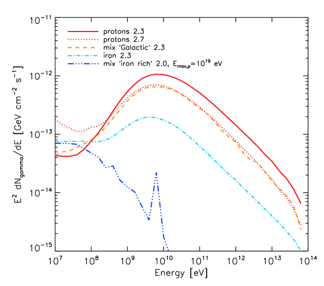
Figure 3: Photon flux produced by synchrotron emission for different source injections. We chose an “anisotropic” distribution of the magnetic field with normalization $B_{0}=1$ nG. The source has a luminosity of $L_{E,19}=10^{42}$ erg s^-1, and is located in the filament described previously, at a distance of 100 Mpc. The average flux integrated over all angular lines of sight are presented.

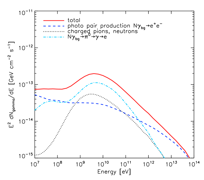
Figure 4: Same as Fig. 3, but for the particular case of a pure iron injection with spectral index 2.3. In red solid lines, the total flux, in blue dashed lines the contribution of the photo-pair production, in black dotted lines the flux due to charged pion production via photo-disintegration processes and to neutron disintegration, in pale blue dash-dotted lines, the contribution of the neutral pion channel.

3 Discussion on detectability

3.1 Synchrotron signal from equal luminosity sources

Our study indicates that around $\sim 10-100\leavevmode\nobreak\$GeV, the gamma ray flux produced by the propagation of ultrahigh energy cosmic rays is fairly robust to changes in composition and in the configuration of magnetic fields. The normalization of the flux ultimately depends on the injected energy, namely, the cosmic ray luminosity and the injection spectral index at the source. The cosmic ray luminosity of the source may be inferred through the normalization to the measured flux of ultrahigh cosmic rays once the source density is specified. The apparent density of ultrahigh energy cosmic ray sources, which coincides with the true source density $n_{\rm s}$ for steady isotropic emitting sources (which we assume here; see Section 4 for a brief discussion of bursting/beamed sources), is bound by the lack of repeaters in the Pierre Auger dataset: $n_{\rm s}\gtrsim 10^{-5}\,$Mpc^-3 (Kashti & Waxman 2008). This lower bound may in turn be translated into an upper limit for the gamma ray flux expected from equal luminosity cosmic ray sources, $L_{E,19}\lesssim 10^{42}\,$erg/s.

Figure 5 presents the spectra obtained for sources of luminosity $L_{E,19}=10^{42}$ erg s^-1 and of number density $n_{\rm s}=10^{-5}$ Mpc^-3. For each case, we represent the median spectrum of 1000 realizations of local source distributions, the minimum distance to a source being of 4 Mpc. Our calculated values are comparable to the cosmic ray fluxes detected by the two most recent experiments: HiRes and the Pierre Auger Observatory. The gamma ray fluxes obtained for single sources with this normalization (i.e. a luminosity of $L_{E,19}=10^{42}$ erg s^-1) at a distance of 100 Mpc are presented in Figs. 2, 3 and 4.

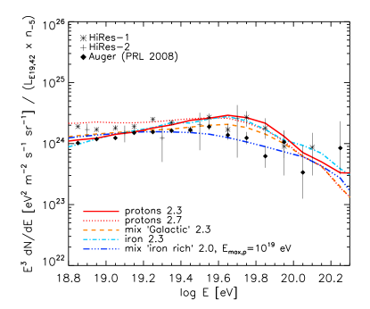
Figure 5: Propagated spectra of ultrahigh energy cosmic rays for various chemical compositions as described in section 2.4 and corresponding spectral indices to best fit the observational data. Sources are assumed to share an equal luminosity $L_{E,19}=10^{42}$ erg s^-1 and a spatial density $n_{\rm s}=10^{-5}$ Mpc^-3.

These gamma ray fluxes lie below the limits of detectability of current and upcoming instruments such as Fermi, HESS or the Cerenkov Telescope Array (CTA), by more than two orders of magnitude. The sensitivity of the Fermi telescope is indeed of order $\sim 2\times 10^{-10}\leavevmode\nobreak\$GeV s^-1 cm^-2 around 10 GeV for a year of observation and the future Cherenkov Telescope Array (CTA) is expected to have a sensitivity of order $\sim 10^{-11}$ GeV $\rm s^{-1}cm^{-2}$ for 100 hours for a point source around TeV energies (Atwood et al. 2009; Wagner et al. 2009).

3.2 Rare and powerful sources

We conclude from the previous subsection that only powerful sources embedded in magnetized environments, rare with respect to the average population of ultrahigh energy cosmic ray sources, may produce a gamma ray signature strong enough to be observed by current and upcoming experiments. In the following, we examine the case of two such sources embedded in filaments, with (isotropic) luminosity chosen to be higher than the average allowed by the cosmic ray normalization for equal luminosity sources: $L_{E,19}=10^{44}$ erg s^-1 and $L_{E,19}=10^{46}$ erg s^-1. As a case study, we place these sources at a distance of $D=100\leavevmode\nobreak\$Mpc and $D=1\leavevmode\nobreak\$Gpc respectively. Those distances are consistent with the number density of objects found at comparable photon luminosities (see for example Wall et al. 2005).

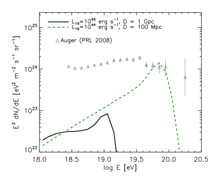
Figure 6: Propagated spectra of ultrahigh energy cosmic rays from a single source with luminosity $L_{E,19}=10^{46}$ erg s^-1 located at a distance of $D=1\leavevmode\nobreak\$Gpc (black solid) or $L_{E,19}=10^{44}$ erg s^-1 and $D=100\leavevmode\nobreak\$Mpc (green dashed). The injection spectral index is 2.0 in both cases. The observed Auger spectrum (Abraham et al. 2008b) is overlaid.

The ultrahigh energy cosmic ray spectra obtained after propagation from these two model sources are represented in Fig. 6. The injection at the source is assumed to be pure proton and with an index of 2.0. The comparison with the Auger data shows that the close-by source (green dashed) is marginally excluded. More precisely, such a source should produce a strong anisotropy signal, of order unity relatively to the all-sky background, if the magnetic deflection at this energy $\sim 7\times 10^{19}\,$eV is smaller than unity. Following Kotera & Lemoine (2008b), the expected deflection is of order $2^{\circ}Z$ if one models the magnetized Universe as a collection of magnetized filaments with $B=10\,$nG ($\lambda_{B}=100\,$kpc) immersed in unmagnetized voids with typical separation $\sim 40\,$Mpc. This estimate neglects the deflection due to the Galactic magnetic field, which depends on incoming direction and charge. Qualitatively speaking, however, one would then expect the above source to produce a strong anisotropy signal unless it injects only iron group nuclei with $Z\sim 26$ at the highest energies. In this latter case, however, the gamma-ray signal would be lower by a factor $\sim 5$ or even suppressed if $E_{\rm max,p}$ is less than the pion production threshold, as discussed in the previous Section. Furthermore, such a source might also give rise to a strong anisotropy at energies $\sim 3\,$EeV, depending on the composition ratio of injected protons to iron group nuclei (Lemoine & Waxman 2009).

On the contrary, the remote source (indicated by the black solid line in Fig. 6) contributes to $\sim 10\%$ of the total flux around $E_{\rm cr}\sim 10^{19}$ eV. Such a source would be wholly invisible in ultrahigh energy cosmic rays, because of the large expected magnetic deflection at this energy, on a large path length of $1\,$Gpc.

Let us now discuss the possibility of detecting these sources in gamma rays. Figure 7 presents our computed images of synchrotron gamma ray emission for these two examples of sources embedded in the filament shown in Fig. 1.

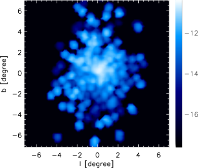
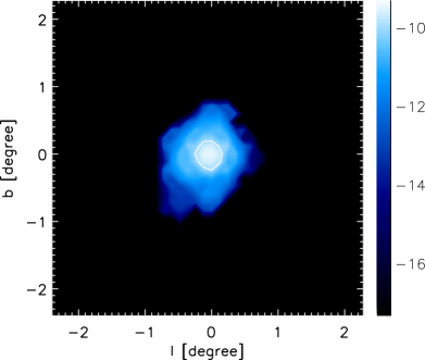
Figure 7: Image of a filament in gamma rays produced via synchrotron emission, integrated over $E_{\gamma}=1-100\leavevmode\nobreak\$GeV. We chose an “anisotropic” distribution of the magnetic field with normalization $B_{0}=1$ nG. Left: the filament is observed along its axis from a distance of 100 Mpc and the embedded source has a cosmic ray luminosity of $L_{E,19}=10^{44}$ erg s^-1. Right: the filament is observed along its axis from a distance of 1 Gpc and the embedded source has a luminosity of $L_{E,19}=10^{46}$ erg s^-1. The color bar indicates the logarithm of the flux in GeV cm^-2 s^-1. White contours indicate a flux level of $10^{-10}\leavevmode\nobreak\$GeV cm^-2 s^-1.

However, one should be aware that the sensitivity of gamma ray telescopes weakens for extended sources by the ratio of the radius of the emission to the angular resolution. Typically, Fermi LAT and HESS have an angular resolution of some fractions of a degree around energies of 10 GeV and 100 GeV respectively. CTA will have an even higher resolution of the order of the arc-minute above 100 GeV. For this reason, one will have to find a source with an acceptable range in luminosity and distance, so as to not lose too much flux due to the angular extension, but still being able to resolve this extension. Let us note that the magnetic configuration around the source should have a negligible role on the flux intensity, as we demonstrated in section 2. However, the magnetic configuration, in particular the strength and the coherence length, directly controls the extension of the image, which is given by the transverse displacement of the protons through magnetic deflection (Gabici & Aharonian 2005).

Figure 8 demonstrates that the synchrotron gamma ray emission from both our model sources could be observed by Fermi LAT and by CTA. Their flux integrated over the angular resolution of these instruments at $\sim 10\leavevmode\nobreak\$GeV are indeed above their corresponding sensitivities. The case presented in dashed green line is however marginally excluded by the observed spectrum of cosmic rays and even more so by the search for anisotropy, as discussed previously (Fig. 6). It thus appears that the gamma ray flux of a source of luminosity $L_{E,19}\sim 10^{44}$ erg s^-1 will be hardly observable, as placing the source at a further distance to reconcile its spectrum with the observations will dilute the gamma ray emission consequently, below the current instrument sensitivities. More promising are extremely powerful sources with $L_{E,19}=10^{46}$ erg s^-1 located around 1 Gpc. According to Fig. 8, the emission from such sources would spread over a fraction of a degree, hence their image could possibly be resolved by Fermi and certainly by CTA.

As discussed in the introduction, the observation of a multi-GeV extended emission as obtained in these images would provide clear evidence for acceleration to ultra-high energies, provided the possible background associated with a halo seeded by TeV photons can be removed. As discussed in  Aharonian et al. (1994), Dai et al. (2002), d’Avezac et al. (2007), Elyiv et al. (2009) and Neronov & Semikoz (2009), the angular size of the latter signal is a rather strong function of the average inter-galactic magnetic field. In particular, if the field is assumed homogeneous and of strength larger than $10^{-14}\,$G, the image is diluted away to large angular scales. Accounting for the inhomogeneity of the magnetic field (see Sec. 3.3 below for a detailed discussion), one concludes that the flux associated to this image, on a degree scale, is to be reduced by the filling factor of voids in which $B\lesssim 10^{-14}\,$G within $\sim 40\,$Mpc of the source (this distance corresponding to the energy loss distance of the primary $\sim 20\,$TeV photons). Furthermore, the angular size of the halo seeded by multi-TeV photons depends strongly on photon energy, i.e. $\delta\theta\propto E_{\gamma}^{-2}$ or $\delta\theta\propto E_{\gamma}^{-1.75}$ depending on $\lambda_{B}$, see Neronov & Semikoz (2009). In contrast, the synchrotron halo is more strongly peaked in energy around $10$ GeV and in this range its angular size is essentially independent of energy, but is rather determined by the magnetic field strength and source distance. Assuming comparable total power in both signals, discrimination should thus be feasible; of course discrimination would be all the more easier if the halo signal seeded by multi-TeV gamma-rays were diluted to large angular scales.

The previous discussion thus indicates that detection might be possible for powerful rare sources at distances in excess of $100\,$Mpc. However, one could not then argue, on the basis of the detection of a gamma ray counterpart that the source of ultrahigh energy cosmic rays has been identified, as this source of gamma-rays must remain a rare event, which could not be considered a representative element of the source population of ultra-high energy cosmic rays. Overall, one finds that this source must contribute to a fraction $10\,$% of the flux at energies well below the GZK cut-off in order to be detectable in gamma-rays. It is important to note that this conclusion does not depend on the degree of beaming of the emission of the source, as we discuss in Section 4.

To conclude this section on a more optimistic note, let us discuss an effect that could improve the prospects for detection. In the above discussion and in our simulations, following Gabici & Aharonian (2005), we have assumed that all of synchrotron emission takes place in the immediate environment of the source, as the magnetic field drops to low values outside the filament, where inverse Compton cascades would therefore become the dominant source of energy loss of the pairs. However, since the typical energy loss length of ultrahigh energy cosmic rays exceeds the typical distance between two filaments, one must in principle allow for the possibility that the beam of ultrahigh energy protons seeds secondary pairs in intervening magnetized filaments, which would then also contribute to the observed synchrotron emission. During the crossing of a filament, ultrahigh energy protons are deflected by an angle $\delta\theta_{i}\,\ll\,1$ (unless the primary cosmic ray carries a large charge or the filament is of unusual magnetisation, see the discussion in Kotera & Lemoine 2008b). Then, as long as the small deflection limit applies, the problem is essentially one-dimensional and each filament contributes to the gamma ray flux a fraction comparable to that of the source environment. The overall synchrotron signal would then be amplified by a factor $\lambda/l_{\rm f}$, where $\lambda$ denotes the relevant energy loss length, $\lambda\sim 100\,$Mpc for pion production of $10^{20}\,$eV protons, $\lambda\sim 1\,$Gpc for pair production of $10^{19}\,$eV protons and $l_{\rm f}\sim 40\,$Mpc is the typical separation between two filaments. Overall, one might expect an amplification as large as an order of magnitude for the contribution to the flux due to pair production, for sources located at several hundreds of Mpc, and a factor of a few for sources located at $100\,$Mpc; and, correspondingly, an amplification factor $\sim 2-3$ for the contribution to the flux due to pion production. Since the pair production channel contributes $\sim 10$% of the total flux at $E_{\gamma}\sim 10-100\leavevmode\nobreak\$GeV for a pure proton composition, the amplification factor should remain limited to a factor of a few, unless the interaction length with magnetized regions is substantially smaller than the above (expected) $l_{\rm f}=40\,$Mpc.

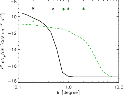
Figure 8: Angular profiles of the images of the sources represented in Fig. 7. We represent the gamma ray flux integrated over energies $E_{\gamma}=1-100\leavevmode\nobreak\$GeV averaged over angular bins, for a filament seen along its axis, at 1 Gpc and $L_{E,19}=10^{46}$ erg s^-1 (black solid line), and at 100 Mpc and $L_{E,19}=10^{44}$ erg s^-1 (green dashed line). The black stars and green crosses present the corresponding integrated flux up to a given angular extension in the sky $\theta$.

3.3 Inverse Compton cascades

Let us briefly discuss the gamma ray signal expected from Compton cascades of ultra-high energy photons and pairs injected in the intergalactic medium. The physics of these cascades has been discussed in detail in Wdowczyk et al. (1972), Protheroe (1986), Protheroe & Stanev (1993), Aharonian et al. (1994), Ferrigno et al. (2004) and Gabici & Aharonian (2007). The angular extent and time distribution of GeV-TeV gamma-rays resulting from inverse Compton cascades seeded by ultra-high energy cosmic rays produced by gamma-ray bursts have also been discussed by Waxman & Coppi (1996). Inverse Compton cascades in the steady state regime have been considered in the study of Armengaud et al. (2006) (for a source located in a cluster of galaxies) but dismissed in the study of Gabici & Aharonian (2005) because of the dilution of the emitted flux through the large deflection of the pairs in the low energy range of the cascade. Indeed, the effective inverse Compton cooling length of electrons of energy $E_{e}\lesssim\,100\,$TeV can be written as $x_{e\gamma}\,\simeq\,3.5\,{\rm kpc}\,(E_{e}/100\,{\rm TeV})^{-1}$ and on this distance scale, the deflection imparted by a magnetic field of coherence length $\lambda_{B}\,\gg\,x_{e\gamma}$ reads $\theta_{e}\,\sim\,x_{e\gamma}/r_{\rm L,e}\,\sim\,3\times 10^{-2}(E_{e}/100\,{\rm TeV})^{-2}(B/10^{-12}\,{\rm G})$. Then, assuming that the last pair of the cascade carries an energy $E_{\rm fin}\,\sim\,20\,$TeV (so that the photon produced through the interaction with the CMB carries a typical energy $\lesssim 1\,$TeV), one finds that a magnetic field larger than $\sim 10^{-12}\,$G isotropizes the low energy cascade, in agreement with the estimates of Gabici & Aharonian (2005).

This situation is modified when one takes into account the inhomogeneous distribution of extra-galactic magnetic fields, as we now discuss. Primary cosmic rays, upon traveling through the voids of large scale structure may inject secondary pairs which undergo inverse Compton cascades in these unmagnetized regions. If the field in such regions is smaller than the above $10^{-12}\,$G, then the cascade will transmit its energy in forward $\lesssim$TeV photons. Of course, depending on the exact value of $B$ where the cascade ends, the resulting image will be spread by some finite angle. Since we are interested in sharply peaked images, let us consider a typical angular size $\theta$ and ignore those regions in which the magnetic field is large enough to give a contribution to the image on a size larger than $\theta$. For $\theta\ll 1$, the problem remains one-dimensional as before, and one can compute the total energy injected in inverse Compton cascades within $\theta$, as follows.

The luminosity injected in secondary pairs and photons up to distance $d$ is written $\chi_{e}L_{\rm cr}(>E)$. Since we are interested in the signatures of ultrahigh cosmic ray sources, we require that $E\geq 10^{19}\,$eV; for protons, the energy loss length due pair production moreover increases dramatically as $E$ becomes smaller than $10^{19}\,$eV, so that the contribution of lower energy particles can be neglected in a first approximation. For photo-pair production, the fraction transfered is $\chi_{e,ee}\simeq d/1\,{\rm Gpc}$ of $L_{E,19}=L_{\rm cr}(>10^{19}\,{\rm eV})$ up to $d\sim 1\,$Gpc. For pion production, the fraction of energy transfered is roughly $\chi_{e,\pi}\simeq d/100\,{\rm Mpc}$ of $L_{\rm cr}(>6\,10^{19}\,{\rm eV})$ in the continuous energy loss approximation. At distances $100\,{\rm Mpc}\,\leq\,d\,\leq\,1\,{\rm Gpc}$, the fraction $\chi_{e}$ of $L_{E,19}$ injected into secondary pairs and photons thus ranges from $\sim 0.5$ for $d=100\,$Mpc to $\sim 1$ at $d=1\,$Gpc; in short, it is expected to be of order unity or slightly less. All the energy injected in this way in sufficiently unmagnetized regions (see below) will be deposited through the inverse Compton cascade in the sub-TeV range, with a typical energy flux dependence $\propto E_{\gamma}^{1/2}$ up to some maximal energy $E_{\gamma,\rm max}\sim 1-10\,$TeV beyond which the Universe is opaque to gamma rays on the distance scale $d$ (Ferrigno et al. 2004). Neglecting any redshift dependence for simplicity, the gamma-ray energy flux per unit energy interval may then be approximated as:

$$E_{\gamma}^{2}\frac{{\rm d}N_{\gamma}}{{\rm d}E_{\gamma}} \,\approx\, f_{\rm 1d}(<B_{\theta})\,\chi_{e}\frac{L_{\rm cr}}{8\pi d^{2}}\left(\frac{E_{\gamma}}{E_{\gamma,\rm max}}\right)^{1/2}$$ (6)

$$\,\simeq\, 2.5\times 10^{-10}\,{\rm GeV}\,{\rm cm}^{-2}\,{\rm s}^{-1}\,f_{\rm 1d}(<B_{\theta})\chi_{e}$$

$$\quad\quad\times\frac{L_{E,19}}{10^{42}\,{\rm erg/s}}\left(\frac{d}{100\,{\rm Mpc}}\right)^{-2}\left(\frac{E_{\gamma}}{E_{\gamma,\rm max}}\right)^{1/2}\ .$$

where $f_{\rm 1d}(<B_{\theta})$ denotes the one-dimensional filling factor, i.e. the fraction of the line of sight in which the magnetic field is smaller than the value $B_{\theta}$ such that the deflection of the low energy cascade is $\theta$. For reference, $B_{\theta}\,\sim\,2\times 10^{-14}\,$G for $\theta\sim 1^{\circ}$. In general, one finds in the literature the three-dimensional filling factor $f_{\rm 3d}$, but $f_{\rm 1d}(<B_{\theta})\sim f_{\rm 3d}(<B_{\theta})$ up to a numerical prefactor of order unity that depends on the geometry of the structures. Interestingly enough, the amount of magnetization of the voids of large scale structure is directly related to the origin of large scale magnetic fields. Obviously, if galactic and cluster magnetic fields originate from a seed field produced in a homogeneous way with a present day strength $B\gg 10^{-14}\,$G, then the above gamma ray flux will be diluted to large angular scales, hence below detection threshold. However, if the seed field, extrapolated to present day values is much lower than this value, or if most of the magnetic enrichment of the intergalactic medium results from the pollution by star forming galaxies and radio-galaxies, then one should expect $f_{\rm 1d}(<B_{\theta})$ to be non negligible. For instance, Donnert et al. (2009) obtain $f_{\rm 3d}(<10^{-14}\,{\rm G})\sim{\cal O}(1)$ in such models. Given the sensitivity of current gamma ray experiments such as H.E.S.S. in the TeV energy range, the inverse Compton cascades might then produce degree-size detectable halos for source luminosities $\gtrsim 10^{43}[f_{\rm 3d}(<10^{-14}\,{\rm G})]^{-1}(d/100\,{\rm Mpc})^{-2}\,$erg/s. For future instruments such as CTA, the detectability condition will be of order $L_{\rm s}\gtrsim 10^{41}[f_{\rm 3d}(<10^{-14}\,{\rm G})]^{-1}(d/100\,{\rm Mpc})^{-2}\,$erg/s. The expected flux level remains quite uncertain as it depends mostly on the configuration of the extragalactic magnetic field in the voids, contrarily to the synchrotron signal which is mainly controlled by the source luminosity.

We note that intergalactic magnetic fields of strength $B\lesssim 10^{-15}\,$G might be probed through the delay time of the high energy afterglow of gamma-ray bursts (Plaga 1995; Ichiki et al. 2008) or the GeV emission around blazars (Aharonian et al. 1994; Dai et al. 2002; d’Avezac et al. 2007; Elyiv et al. 2009; Neronov & Semikoz 2009), as discussed earlier. As the present paper was being refereed, some first estimates on lower bounds for the average magnetic field appeared, giving $B\gtrsim 10^{-16}-10^{-15}$ G, see Neronov & Vovk (2010), Ando & Kusenko (2010) and Dolag et al. (2010).

3.4 Cen A

In view of the results of section 3.1, one may want to consider also the case of mildly powerful but nearby sources. One such potential source is Cen A, which has attracted a considerable amount of attention, as it is the nearest radio-galaxy (3.8 Mpc) and more recently, because a fraction of the Pierre Auger events above $60\,$EeV have clustered within $10-20^{\circ}$ of this source. As discussed in detail in Lemoine & Waxman (2009), this source is likely too weak to accelerate protons to $\gtrsim 10^{19}\,$eV in steady state, but heavy nuclei might possibly be accelerated up to GZK energies. The acceleration of protons to ultrahigh energies in flaring episodes of high luminosity has been proposed in Dermer et al. (2009). It is also important to recall that the apparent clustering in this direction can be naturally explained thanks to the large concentration of matter in the local Universe, in the direction of Cen A but located further away. As discussed in Lemoine & Waxman (2009), some of the events detected toward Cen A could also be attributed to rare and powerful bursting sources located in the Cen A host galaxy, such as gamma-ray bursts. Due to the scattering of the particles on the magnetized lobes, one would not be able to distinguish such bursting sources from a source located in the core of Cen A.

We have argued throughout this paper that a clear signature of ultrahigh energy cosmic ray propagation could be produced in presence of an extended and strong magnetized region around the source. The magnetized lobes of Cen A provide such a site, with an extension of $R_{\rm lobe}\sim 100\leavevmode\nobreak\$kpc, and a magnetic field of average intensity $B_{\rm lobe}\sim 1\leavevmode\nobreak\ \mu$G and coherence length $\lambda_{\rm lobe}\sim 20\leavevmode\nobreak\$kpc (Feain et al. 2009). In terms of gamma ray fluxes, one can calculate however that the only advantage Cen A presents compared to average types of sources described in section 3.1 lies in its proximity. As noted before, the bulk of gamma ray emission will be due to electrons and positrons produced by pion production with $E_{e}>10^{19}$ eV. The flux of these secondary electron/positron emission scales as the distance $r$ the primary protons travels through, as long as $r\ll\lambda$, with $\lambda$ the energy loss length by pion production. In our situation, in order to calculate the synchrotron gamma ray flux, this distance corresponds to the size of the magnetized structure with $B\gtrsim 0.5\,\mbox{nG}\,(E_{e}/10^{19}\,{\rm eV})^{-3/4}$, namely $r\sim R_{\rm lobe}$ in our toy-model. One may also note that considering the magnetic field strength in the lobes, the gamma ray flux will peak around $E_{\gamma\rm syn}\sim 6.8\,$TeV$\,B_{\rm lobe}E_{e,19}^{2}$, according to Eq. 2. Scaling the expected flux from the lobes around $10\leavevmode\nobreak\$TeV $F_{\rm lobe,10\,TeV}$ to the flux that we calculated in section 3.1 for standard sources embedded in filaments around $10\leavevmode\nobreak\$GeV $F_{\rm fil,10\,GeV}$, one obtains:

$$F_{\rm lobe,10\,TeV} \sim \left(\frac{d_{\rm Cen\,A}}{d_{\rm fil}}\right)^{-2}\,\frac{L_{\rm CenA}}{10^{42}\,{\rm erg/s}}\,\frac{R_{\rm lobe}}{5\,{\rm Mpc}}\,F_{\rm fil,10\,GeV}$$ (7)

$$\sim 2\times 10^{-14}\leavevmode\nobreak\ \mbox{GeV}\leavevmode\nobreak\ \mbox{s}^{-1}\mbox{cm}^{-2}\,,$$ (8)

which is far below current instrument sensitivities. Here, $d_{\rm CenA}=3.8\leavevmode\nobreak\$Mpc and $d_{\rm fil}=100$ Mpc are the distance of Cen A and of our model filament respectively, and $L_{\rm CenA}$ is the cosmic ray luminosity of Cen A which we set to $10^{39}$ erg s^-1 according to constraints from ultrahigh energy cosmic ray observations (see for example Hardcastle et al. 2009). Moreover, Cen A covers $\theta_{\rm source}\sim 10^{\circ}$ in the sky, inducing a sensitivity loss of a factor $\theta_{\rm source}/\theta_{\rm PSF}\sim 10$ for the Fermi telescope ($\theta_{\rm PSF}$ represents the angular resolution of the instrument).

All in all, taking into account all these disadvantages, we conclude that the synchrotron emission produced in the lobes of Cen A would be three orders of magnitudes weaker than the flux obtained for the average types of sources described in section 3.1.

Our numerical estimate using the method introduced in section 2.2 and modeling the lobes as spherical uniformly magnetized structures confirms this calculation. We note that the contribution of the pair production channel is not as suppressed as the other components. Due to the strength of the magnetic field, the electrons and positrons radiating in synchrotron around $0.1-1\leavevmode\nobreak\$GeV are of lower energy than for the standard filament case ($E_{e}\sim 10\leavevmode\nobreak\$MeV) and thus are more numerous. At these energies, the synchrotron emission in the filament was also partially suppressed by the shortening of the inverse Compton loss length as compared to the synchrotron loss length. Because of the high magnetic field intensity, this effect is less pronounced in the lobe case.

Recently Fermi LAT discovered a gamma ray emission emanating from the giant radio lobes of Cen A (Cheung et al. 2010). In light of our discussion, the ultrahigh energy cosmic ray origin of this emission can be excluded. It could rather be interpreted as an inverse Compton scattered relic radiation on the CMB and infrared and optical photon backgrounds, as proposed by Cheung et al. (2010).

Let us note additionally that Kachelrieß et al. (2009) have provided estimates for gamma ray fluxes emitted as a result of the production of ultrahigh energy cosmic rays in Cen A. These authors conclude that a substantial signal could be produced, well within the detection capabilities of Fermi and CTA. However this signal results from interactions of cosmic rays accelerated inside the source, not outside. As we discussed before, such a gamma ray signal, i.e. that could not be angularly resolved from the source, could not be interpreted without ambiguity. In particular, one would not be able to discriminate it from a secondary signal produced by multi-TeV leptons or hadrons accelerated in the same source. Furthermore, the gamma ray signal discussed in Kachelrieß et al. (2009) is mainly attributed to cosmic rays at energies $\lesssim 10^{18}\,$eV, not to ultrahigh cosmic rays above the ankle, although the generation spectrum in the source is normalized to the Pierre Auger Observatory events at $\gtrsim 6\times 10^{19}\,$eV. The conclusions thus depend rather strongly on the shape of the injection spectrum as well as on the phenomenological modelling of acceleration, as made clear by Fig. 1 of their study.

Finally one may turn to the highest energies and search for ultrahigh energy cosmic ray signatures from Cen A by looking directly at the ultrahigh energy secondary photons produced during the propagation. These photons should indeed not experience cascading at this close distance. Taylor et al. (2009) have studied this potential signature and concluded that Auger should be able to detect $0.05-0.075$ photon per year from Cen A, assuming that it is responsible for 10% of the $>6\times 10^{19}$ eV cosmic ray flux, and assuming a 25% efficiency for photon discrimination.

4 Discussion and conclusions

Let us first recap our main findings. We have discussed the detectability of gamma ray halos of ultrahigh energy cosmic ray sources, relaxing most of the assumptions made in previous studies. We have focused our study on the synchrotron signal emitted by secondary pairs, which offers a possibility of unambiguous detection. In this study, we have taken into account the inhomogeneous distribution of the magnetic field in the source environment and examined the effects of non pure proton composition on the gamma ray signal. We find that the gamma ray flux predictions are rather robust with respect to the uncertainties attached to these physical parameters. The normalization and hence the detectability of this flux ultimately depends on the energy injected in the primary cosmic rays, for realistic values of the magnetic field. We have further demonstrated that the average type of sources contributing to the ultrahigh energy cosmic ray spectrum produces a gamma ray flux more than two orders of magnitudes lower than the sensitivity of the current and upcoming instruments. The case of rare powerful sources contributing to more than 10% of the cosmic ray flux is far more promising in terms of detectability. We have found that gamma ray signatures of those sources could be detectable provided that they are located far enough not to overshoot the observed cosmic ray spectrum. If the extended emission of such signatures were resolved (which should be the case with Fermi and CTA), such a detection would provide a distinctive proof of acceleration of cosmic rays to energies $\gtrsim 10^{19}\,$eV. However, as we have discussed, such gamma ray sources should remain exceptional and could not be considered as representatives of the population of ultrahigh energy cosmic ray sources. We have also discussed the deflection and the dilution of the Compton cascading gamma ray signal at sub-TeV energies. In this case, the flux prediction depends sensitively on the filling factor of the magnetic field with values smaller smaller than $\sim 10^{-14}\,$G in the voids of large scale structure. If this latter is larger than a few percents, as suggested by some scenarios of the origin of cosmic magnetic fields, then the inverse Compton cascade could provide a degree size image of the ultra-high cosmic ray source, with a flux slightly larger than that associated to the synchrotron component.

Finally, we have also discussed the detection of nearby sources, considering the radiogalaxy Centaurus A as a protoypical example. We have demonstrated that, if ultrahigh energy cosmic rays are produced in Cen A, their secondary gamma ray halo signature should not be detectable by current experiments. Our conclusion indicates in particular that the gamma ray emission detected by Fermi LAT from the giant radio lobes of Cen A (Cheung et al. 2010) cannot result from the synchrotron radiation of ultrahigh energy secondaries in that source.

We need to stress that, in our discussion, we have systematically assumed that the source was emitting cosmic rays at a steady rate with isotropic output. Let us discuss these assumptions. If the source is rather of the flaring type, then, at a same cosmic ray source luminosity, the flux predictions will be reduced by the ratio of the source flare duration $\Delta t$ to the dispersion in arrival times $\sigma_{t}$ that results from propagation in intergalactic magnetic fields. In theoretical models, $\Delta t$ can take values ranging from a few seconds for gamma-ray bursts (Milgrom & Usov 1996; Waxman 1995; Vietri 1995) to days in the case of blazar flares, while $\sigma_{t}$ is typically expected to be of the order of $10^{3}-10^{5}\,$yrs for protons of energy $\gtrsim 70\,$EeV (see Kotera & Lemoine 2008b for a detailed discussion). In both cases, the large luminosity during the flaring episodes is not sufficient to compensate for the dilution in arrival times. Of course, if the source is a repeater, with a timescale between two flaring episodes shorter than the intergalactic dispersion timescale, then one recovers a steady emitting situation, with an effective luminosity reduced by the fraction of time during which the source is active.

This latter situation may well apply to powerful radio-galaxies that produce ultra-high energy cosmic rays with flaring activity, since the size and magnetization of the jets and lobes are sufficient to deflect ultra-high energy cosmic rays by an angle of order unity, theredy dispersing them in time over $\sim R_{\rm lobe}/c\sim 3\times 10^{5}\,$yr, with $R_{\rm lobe}\sim 100\,$kpc the typical transverse scale of the lobes. Even if ultra-high energy cosmic rays are ejected as neutrons, as discussed for instance by Dermer et al. (2009), a substantial fraction of these cosmic rays will suffer dispersion as the decay length of neutrons of energy $E_{n}$ is $0.9(E_{n}/10^{20}\,{\rm eV})\,$Mpc. In such a configuration, the source would effectively emit its cosmic rays isotropically, as we have assumed.

Let us nonetheless discuss the case of beamed sources, for the sake of completeness. If one considers a single source, emitting cosmic rays in a solid angle $\Delta\Omega_{\rm s}<4\pi$, then at a same total luminosity as an isotropic source, the luminosity emitted per steradian is larger by $4\pi/\Delta\Omega_{\rm s}$ and so is the expected gamma-ray flux (in the limit of small deflection around the source, which is necessary for detection). In other words, the required total cosmic-ray luminosity per source for detection of gamma rays is lowered by a factor $\Delta\Omega_{\rm s}/(4\pi)$. However, at a fixed contribution of the source to the cosmic ray flux, the expected gamma-ray flux does not depend on the beaming angle. This is because both the cosmic ray flux and the gamma-ray flux are determined by the number of visible sources times the luminosity per steradian. In particular, our conclusion that a source must contribute to more than 10% of the ultra-high energy cosmic ray flux in order for the synchrotron signal to be detectable remains unchanged if $\Delta\Omega_{\rm s}<4\pi$.

5 Acknowledgement

We thank Eric Armengaud, Stefano Gabici, Susumu Inoue, Simon Prunet and Michael Punch for helpful discussions. We thank Christophe Pichon for helping us identify adequate filaments in our cosmological simulation cube using his skeleton program, and Stéphane Colombi for providing us with the Dark Matter cosmological simulation cube. KK is supported by the NSF grant PHY-0758017 and by Kavli Institute for Cosmological Physics at the University of Chicago through grant NSF PHY-0551142 and an endowment from the Kavli Foundation.

References

- Abbasi et al. (2010) Abbasi, R. U., Abu-Zayyad, T., Al-Seady, M., et al. 2010, Physical Review Letters, 104, 161101
- Abbasi et al. (2005) Abbasi, R. U. et al. 2005, ApJ, 622, 910
- Abraham et al. (2007) Abraham, J. et al. 2007, Science, 318, 938
- Abraham et al. (2008a) Abraham, J. et al. 2008a, Astroparticle Physics, 29, 188
- Abraham et al. (2008b) Abraham, J. et al. 2008b, Physical Review Letters, 101, 061101
- Abraham et al. (2009) Abraham, J. et al. 2009, ArXiv: 0906.2319
- Abraham et al. (2010) Abraham, J. et al. 2010, Phys. Rev. Lett., 104, 091101
- Aharonian (2002) Aharonian, F. A. 2002, MNRAS, 332, 215
- Aharonian et al. (1994) Aharonian, F. A., Coppi, P. S., & Voelk, H. J. 1994, ApJ, 423, L5
- Aharonian et al. (2010) Aharonian, F. A., Kelner, S. R., & Prosekin, A. Y. 2010, Phys. Rev. D, 82, 043002
- Allard et al. (2006) Allard, D., Ave, M., Busca, N., et al. 2006, Journal of Cosmology and Astro-Particle Physics, 9, 5
- Allard et al. (2008) Allard, D., Busca, N. G., Decerprit, G., Olinto, A. V., & Parizot, E. 2008, Journal of Cosmology and Astro-Particle Physics, 10, 33
- Ando & Kusenko (2010) Ando, S. & Kusenko, A. 2010, Phys. Rev. D, 81, 113006
- Armengaud et al. (2006) Armengaud, E., Sigl, G., & Miniati, F. 2006, Phys. Rev. D, 73, 083008
- Atwood et al. (2009) Atwood, W. B. et al. 2009, ApJ, 697, 1071
- Berezinsky et al. (2006) Berezinsky, V., Gazizov, A., & Grigorieva, S. 2006, Phys. Rev. D, 74, 043005
- Bird et al. (1993) Bird, D. J. et al. 1993, Physical Review Letters, 71, 3401
- Casse et al. (2002) Casse, F., Lemoine, M., & Pelletier, G. 2002, Phys. Rev., D65, 023002
- Cheung et al. (2010) Cheung, C. C., Fukazawa, Y., Knödlseder, J., Stawarz, L., & Fermi-LAT collaboration. 2010, in Bulletin of the American Astronomical Society, Vol. 41, Bulletin of the American Astronomical Society, 440–+
- Clark et al. (1970) Clark, T. A., Brown, L. W., & Alexander, J. K. 1970, Nature, 228, 847
- Dai et al. (2002) Dai, Z. G., Zhang, B., Gou, L. J., Mészáros, P., & Waxman, E. 2002, ApJ, 580, L7
- Das et al. (2008) Das, S., Kang, H., Ryu, D., & Cho, J. 2008, ApJ, 682, 29
- d’Avezac et al. (2007) d’Avezac, P., Dubus, G., & Giebels, B. 2007, Astron. Astrophys., 469, 857
- Dermer et al. (2009) Dermer, C. D., Razzaque, S., Finke, J. D., & Atoyan, A. 2009, New Journal of Physics, 11, 065016
- Dolag (2006) Dolag, K. 2006, Astronomische Nachrichten, 327, 575
- Dolag et al. (2004) Dolag, K., Grasso, D., Springel, V., & Tkachev, I. 2004, Journal of Korean Astronomical Society, 37, 427
- Dolag et al. (2005) Dolag, K., Grasso, D., Springel, V., & Tkachev, I. 2005, Journal of Cosmology and Astro-Particle Physics, 1, 9
- Dolag et al. (2010) Dolag, K., Kachelriess, M., Ostapchenko, S., & Tomas, R. 2010, ArXiv e-prints
- Donnert et al. (2009) Donnert, J., Dolag, K., Lesch, H., & Müller, E. 2009, MNRAS, 392, 1008
- Elyiv et al. (2009) Elyiv, A., Neronov, A., & Semikoz, D. V. 2009, Phys. Rev. D, 80, 023010
- Feain et al. (2009) Feain, I. J., Ekers, R. D., Murphy, T., et al. 2009, ApJ, 707, 114
- Ferrigno et al. (2004) Ferrigno, C., Blasi, P., & de Marco, D. 2004, Nuclear Physics B Proceedings Supplements, 136, 191
- Gabici & Aharonian (2005) Gabici, S. & Aharonian, F. A. 2005, Physical Review Letters, 95, 251102
- Gabici & Aharonian (2007) Gabici, S. & Aharonian, F. A. 2007, Ap&SS, 309, 465
- Gould & Rephaeli (1978) Gould, R. J. & Rephaeli, Y. 1978, ApJ, 225, 318
- Gould & Schréder (1967) Gould, R. J. & Schréder, G. P. 1967, Physical Review, 155, 1408
- Hardcastle et al. (2009) Hardcastle, M. J., Cheung, C. C., Feain, I. J., & Stawarz, Ł. 2009, MNRAS, 393, 1041
- Ichiki et al. (2008) Ichiki, K., Inoue, S., & Takahashi, K. 2008, ApJ, 682, 127
- Kachelrieß et al. (2009) Kachelrieß, M., Ostapchenko, S., & Tomàs, R. 2009, New Journal of Physics, 11, 065017
- Kashti & Waxman (2008) Kashti, T. & Waxman, E. 2008, Journal of Cosmology and Astro-Particle Physics, 5, 6
- Kelner & Aharonian (2008) Kelner, S. R. & Aharonian, F. A. 2008, Phys. Rev. D, 78, 034013
- King & Coles (2006) King, E. J. & Coles, P. 2006, MNRAS, 365, 1288
- Kotera et al. (2009) Kotera, K., Allard, D., Murase, K., et al. 2009, ArXiv e-prints
- Kotera & Lemoine (2008a) Kotera, K. & Lemoine, M. 2008a, Phys. Rev. D, 77, 023005
- Kotera & Lemoine (2008b) Kotera, K. & Lemoine, M. 2008b, Phys. Rev. D, 77, 123003
- Lee (1998) Lee, S. 1998, Phys. Rev. D, 58, 043004
- Lemoine & Waxman (2009) Lemoine, M. & Waxman, E. 2009, JCAP, 0911, 009
- Milgrom & Usov (1996) Milgrom, M. & Usov, V. 1996, Astroparticle Physics, 4, 365
- Mücke et al. (1999) Mücke, A., Rachen, J. P., Engel, R., Protheroe, R. J., & Stanev, T. 1999, Publications of the Astronomical Society of Australia, 16, 160
- Neronov & Semikoz (2009) Neronov, A. & Semikoz, D. V. 2009, Phys. Rev. D, 80, 123012
- Neronov & Vovk (2010) Neronov, A. & Vovk, I. 2010, Science, 328, 73
- Plaga (1995) Plaga, R. 1995, Nature, 374, 430
- Protheroe (1986) Protheroe, R. J. 1986, MNRAS, 221, 769
- Protheroe & Stanev (1993) Protheroe, R. J. & Stanev, T. 1993, MNRAS, 264, 191
- Ryu et al. (1998) Ryu, D., Kang, H., & Biermann, P. L. 1998, A&A, 335, 19
- Sigl et al. (2004) Sigl, G., Miniati, F., & Enßlin, T. A. 2004, Phys. Rev. D, 70, 043007
- Stecker (1973) Stecker, F. W. 1973, Ap&SS, 20, 47
- Stecker et al. (2006) Stecker, F. W., Malkan, M. A., & Scully, S. T. 2006, ApJ, 648, 774
- Taylor et al. (2009) Taylor, A. M., Hinton, J. A., Blasi, P., & Ave, M. 2009, Physical Review Letters, 103, 051102
- Unger et al. (2007) Unger, M., Engel, R., Schüssler, F., Ulrich, R., & Pierre AUGER Collaboration. 2007, Astronomische Nachrichten, 328, 614
- Vietri (1995) Vietri, M. 1995, ApJ, 453, 883
- Wagner et al. (2009) Wagner, R. M., Lindfors, E. J., Sillanpää, A., et al. 2009, ArXiv e-prints
- Wall et al. (2005) Wall, J. V., Jackson, C. A., Shaver, P. A., Hook, I. M., & Kellermann, K. I. 2005, A&A, 434, 133
- Waxman (1995) Waxman, E. 1995, Physical Review Letters, 75, 386
- Waxman & Bahcall (1999) Waxman, E. & Bahcall, J. N. 1999, Phys. Rev., D59, 023002
- Waxman & Coppi (1996) Waxman, E. & Coppi, P. 1996, ApJ, 464, L75+
- Wdowczyk et al. (1972) Wdowczyk, J., Tkaczyk, W., & Wolfendale, A. W. 1972, Journal of Physics A Mathematical General, 5, 1419