The mass-$L_{x}$ relation for moderate luminosity X-ray clusters

Abstract

We present measurements of the masses of a sample of 25 moderate X-ray luminosity clusters of galaxies from the 160 square degree ROSAT survey. The masses were obtained from a weak lensing analysis of deep $F814W$ images obtained using the Advanced Camera for Surveys (ACS). We present an accurate empirical correction for the effect of charge transfer (in)efficiency on the shapes of faint galaxies. A significant lensing signal is detected around most of the clusters. The lensing mass correlates tightly with the cluster richness. We measured the intrinsic scatter in the scaling relation between $M_{2500}$ and $L_{X}$ to be $\sigma_{\log{L_{X}|M}}=0.23^{+0.10}_{-0.04}$. The best fit power law slope and normalisation are found to be $\alpha=0.68\pm 0.07$ and $M_{X}=(1.2\pm 0.12)\times h_{70}^{-1}10^{14}\hbox{$\rm{M}_{\odot}$}$ (for $L_{X}=2\times 10^{44}h_{70}^{-2}$ erg/s). These results agree well with a number of recent studies, but the normalisation is lower compared to the study of Rykoff et al. (2008a). One explanation for this difference may be the fact that (sub)structures projected along the line-of-sight boost both the galaxy counts and the lensing mass. Such superpositions lead to an increased mass at a given $L_{X}$ when clusters are binned by richness.

1. Introduction

Clusters of galaxies are known to exhibit correlations between their various observable properties, such as the well-known relation between X-ray luminosity and X-ray temperature. These scaling relations are the result of the various processes that govern the formation and subsequent evolution of galaxy clusters. Hence, the study of cluster scaling laws provides the basis of testing models for the formation of clusters of galaxies and of galaxies themselves. For instance, N-body codes can nowadays reliably and robustly predict the evolution of the mass function of cluster halos (e.g., Evrard et al., 2002). Hydrodynamic simulations and semi-analytic techniques then allow us to predict the X-ray and optical appearance of these halos (e.g., Voit, 2005; Nagai et al., 2007; Bower et al., 2008).

The mean relation and the intrinsic dispersion of the resulting mass-observable relations provide a test of the adequacy of the physical processes included in the simulations: a realistic simulation should reproduce the mean relation, the intrinsic scatter, and its evolution (if any). Such comparisons have recently led to the realization that cluster simulations must include radiative cooling and feedback from supernovae and AGNs in order to successfully explain the observed scaling relations (see Voit (2005) for a review). While the core regions of clusters remain difficult to model accurately, high-resolution simulations with cooling and feedback now produce clusters whose X-ray properties agree well with those of observed clusters outside the central 100 kpc or so (Nagai et al., 2007).

An empirically determined mass scaling relation is not only useful to directly test our understanding of cluster physics, it also allows one to relate the observables directly to the mass of cluster-sized halos. The latter, for instance, enables one to transform the observed luminosity function into a mass function, which in turn can be compared to different cosmological models. Such studies have already provided interesting constraints on cosmological parameters which complement constraints from other probes (e.g., Henry, 2000; Borgani et al., 2001; Reiprich & Böhringer, 2002; Henry, 2004; Gladders et al., 2007; Henry et al., 2009; Vikhlinin et al., 2009b; Mantz et al., 2010b).

To determine cluster masses, a number of methods are available. Dynamical techniques, such as the assumption of hydrostatic equilibrium in X-ray observations, have been widely used. The inferred masses, however, are likely to be systematically underestimated by up to $20\%$ because of pressure support from turbulence and energy input from active galactic nuclei (e.g., Evrard et al., 1996; Rasia et al., 2006; Nagai et al., 2007). Masses derived from weak gravitational lensing do not require assumptions about the dynamical state of the cluster and can in principle be compared directly to the outcome of numerical simulations. It is worth noting, however, that lensing is sensitive to all structure along the line-of-sight. Weak lensing is now a well-established technique (for a review see Hoekstra & Jain, 2008) and recent work has indeed provided support for non-hydrostatic gas in the outskirts of X-ray luminous clusters of galaxies (Mahdavi et al., 2008).

To date, most work has focussed on the most massive clusters at intermediate redshifts (e.g., Bardeau et al., 2007; Hoekstra, 2007; Zhang et al., 2008), because of the relatively large lensing signal. In this paper we focus on extending the mass range towards clusters with lower X-ray luminosities ($L_{x}<{\rm few~{}}10^{44}$ erg/s). To detect the lensing signal of these lower mass clusters, the number density of lensed background galaxies needs to be increased significantly, compared to deep ground based observations. The reason for this requirement is that the error in the weak lensing mass estimate is set by the intrinsic shapes of the galaxies and their number density.

To this end, we have conducted a weak-lensing analysis on images obtained during a snapshot survey of 25 moderate luminosity X-ray clusters with the Advanced Camera for Surveys (ACS) on board the Hubble Space Telescope (HST). These clusters were randomly selected from the ROSAT 160 Square Degree (160SD) Cluster Catalog (Mullis et al., 2003; Vikhlinin et al., 1998). The clusters in the 160SD sample were serendipitously discovered in pointed, relatively wide-field (30’ diameter) observations of the Position-Sensitive Proportional Counter (PSPC) on board the ROSAT X-ray observatory (1990-1999). Seventy-two X-ray clusters between $z=0.3-0.7$ were discovered (see Fig. 1). All have been identified and assigned redshifts (Mullis et al., 2003). Because this survey included pointed observations that were quite long, some of these clusters are among the faintest clusters of galaxies known at these moderately high redshifts. Therefore, our new weak lensing measurements extend the X-ray luminosity limit of the mass-$L_{x}$ relation by almost an order of magnitude, based on targeted observations. We note that studies of the ensemble-averaged properties of clusters discovered in the SDSS (Rykoff et al., 2008a) and X-ray groups in COSMOS (Leauthaud et al., 2010) have pushed the limits to even lower luminosities.

The structure of the paper follows. In §2 we describe our data and weak lensing analysis. In particular we discuss how we correct for the effects of CTE in our ACS data and how we correct for PSF anisotropy. The measurements of the cluster masses, and the comparison to the X-ray properties are presented in §3. We compare our results to previous work and examine biases in our mass estimates that arise from uncertainties in the position of the cluster center and sample selection. Throughout this paper we assume a flat $\Lambda$CDM cosmology with $\Omega_{m}=0.3$ and $H_{0}=70h_{70}$ km/s/Mpc.

Table 1Summary of the observational data for the cluster sample

name	number	$z$	$L_{X}$	RAX-ray	DECX-ray	RABCG	DECBCG	$Q_{\rm BCG}$	$\langle\beta\rangle$	$\langle\beta^{2}\rangle$
(1)	(2)	(3)	(4)	(5)	(6)	(7)	(8)	(9)	(10)	(11)
RXJ$0056.9-2740$	6	0.563	1.14	$00^{h}56^{m}56.1^{s}$	$-27^{\circ}40^{\prime}12^{\prime\prime}$	$00^{h}56^{m}56.98^{s}$	$-27^{\circ}40^{\prime}29.9^{\prime\prime}$	2	0.42	0.23
RXJ$0110.3+1938$	8	0.317	0.40	$01^{h}10^{m}18.0^{s}$	$+19^{\circ}38^{\prime}23^{\prime\prime}$	$01^{h}10^{m}18.22^{s}$	$+19^{\circ}38^{\prime}19.4^{\prime\prime}$	0	0.61	0.43
RXJ$0154.2-5937$	20	0.360	0.90	$01^{h}54^{m}14.8^{s}$	$-59^{\circ}37^{\prime}48^{\prime\prime}$	$01^{h}54^{m}13.72^{s}$	$-59^{\circ}37^{\prime}31.0^{\prime\prime}$	1	0.57	0.38
RXJ$0522.2-3625$	41	0.472	2.07	$05^{h}22^{m}14.2^{s}$	$-36^{\circ}25^{\prime}04^{\prime\prime}$	$05^{h}22^{m}15.48^{s}$	$-36^{\circ}24^{\prime}56.1^{\prime\prime}$	1	0.48	0.29
RXJ$0826.1+2625$	52	0.351	0.65	$08^{h}26^{m}06.4^{s}$	$+26^{\circ}25^{\prime}47^{\prime\prime}$	$08^{h}26^{m}09.45^{s}$	$+26^{\circ}25^{\prime}03.1^{\prime\prime}$	0	0.58	0.39
RXJ$0841.1+6422$	56	0.342	1.60	$08^{h}41^{m}07.4^{s}$	$+64^{\circ}22^{\prime}43^{\prime\prime}$	$08^{h}41^{m}07.65^{s}$	$+64^{\circ}22^{\prime}26.0^{\prime\prime}$	2	0.59	0.40
RXJ$0847.1+3449$	59	0.560	1.17	$08^{h}47^{m}11.3^{s}$	$+34^{\circ}49^{\prime}16^{\prime\prime}$	$08^{h}47^{m}11.79^{s}$	$+34^{\circ}48^{\prime}51.8^{\prime\prime}$	1	0.42	0.23
RXJ$0910.6+4248$	69	0.576	1.44	$09^{h}10^{m}39.7^{s}$	$+42^{\circ}48^{\prime}41^{\prime\prime}$	$09^{h}10^{m}40.53^{s}$	$+42^{\circ}49^{\prime}59.1^{\prime\prime}$	-1	0.41	0.23
RXJ$0921.2+4528$	70	0.315	1.40	$09^{h}21^{m}13.4^{s}$	$+45^{\circ}28^{\prime}50^{\prime\prime}$	$09^{h}21^{m}13.46^{s}$	$+45^{\circ}28^{\prime}56.1^{\prime\prime}$	1	0.61	0.43
RXJ$0926.6+1242$	71	0.489	2.04	$09^{h}26^{m}36.6^{s}$	$+12^{\circ}42^{\prime}56^{\prime\prime}$	$09^{h}26^{m}36.70^{s}$	$+12^{\circ}43^{\prime}03.8^{\prime\prime}$	2	0.47	0.28
RXJ$0957.8+6534$	80	0.530	1.39	$09^{h}57^{m}53.2^{s}$	$+65^{\circ}34^{\prime}30^{\prime\prime}$	$09^{h}57^{m}51.22^{s}$	$+65^{\circ}34^{\prime}25.1^{\prime\prime}$	2	0.44	0.25
RXJ$1015.1+4931$	88	0.383	0.78	$10^{h}15^{m}08.5^{s}$	$+49^{\circ}31^{\prime}32^{\prime\prime}$	$10^{h}15^{m}08.44^{s}$	$+49^{\circ}31^{\prime}50.8^{\prime\prime}$	2	0.55	0.36
RXJ$1117.2+1744$	96	0.305	0.54	$11^{h}17^{m}12.0^{s}$	$+17^{\circ}44^{\prime}24^{\prime\prime}$	$11^{h}17^{m}11.23^{s}$	$+17^{\circ}44^{\prime}00.5^{\prime\prime}$	2	0.62	0.44
RXJ$1117.4+0743$	97	0.477	0.76	$11^{h}17^{m}26.1^{s}$	$+07^{\circ}43^{\prime}35^{\prime\prime}$	$11^{h}17^{m}26.04^{s}$	$+07^{\circ}43^{\prime}38.3^{\prime\prime}$	1	0.48	0.29
RXJ$1123.1+1409$	101	0.340	1.01	$11^{h}23^{m}10.2^{s}$	$+14^{\circ}09^{\prime}44^{\prime\prime}$	$11^{h}23^{m}10.95^{s}$	$+14^{\circ}08^{\prime}36.4^{\prime\prime}$	1	0.59	0.40
RXJ$1354.2-0221$	151	0.546	1.53	$13^{h}54^{m}16.9^{s}$	$-02^{\circ}21^{\prime}47^{\prime\prime}$	$13^{h}54^{m}17.19^{s}$	$-02^{\circ}21^{\prime}59.2^{\prime\prime}$	2	0.43	0.24
RXJ$1524.6+0957$	170	0.516	3.94	$15^{h}24^{m}40.3^{s}$	$+09^{\circ}57^{\prime}39^{\prime\prime}$	$15^{h}24^{m}41.56^{s}$	$+09^{\circ}57^{\prime}34.3^{\prime\prime}$	1	0.45	0.26
RXJ$1540.8+1445$	172	0.441	0.81	$15^{h}40^{m}53.3^{s}$	$+14^{\circ}45^{\prime}34^{\prime\prime}$	$15^{h}40^{m}53.96^{s}$	$+14^{\circ}45^{\prime}56.0^{\prime\prime}$	1	0.51	0.31
RXJ$1642.6+3935$	186	0.355	0.62	$16^{h}42^{m}38.9^{s}$	$+39^{\circ}35^{\prime}53^{\prime\prime}$	$16^{h}42^{m}38.35^{s}$	$+39^{\circ}36^{\prime}10.4^{\prime\prime}$	1	0.58	0.39
RXJ$2059.9-4245$	199	0.323	2.44	$20^{h}59^{m}55.2^{s}$	$-42^{\circ}45^{\prime}33^{\prime\prime}$	$20^{h}59^{m}54.92^{s}$	$-42^{\circ}45^{\prime}32.1^{\prime\prime}$	2	0.61	0.42
RXJ$2108.8-0516$	200	0.319	0.81	$21^{h}08^{m}51.2^{s}$	$-05^{\circ}16^{\prime}49^{\prime\prime}$	$21^{h}08^{m}51.17^{s}$	$-05^{\circ}16^{\prime}58.4^{\prime\prime}$	2	0.61	0.42
RXJ$2139.9-4305$	203	0.376	0.59	$21^{h}39^{m}58.5^{s}$	$-43^{\circ}05^{\prime}14^{\prime\prime}$	$21^{h}39^{m}58.22^{s}$	$-43^{\circ}05^{\prime}13.9^{\prime\prime}$	2	0.56	0.37
RXJ$2146.0+0423$	204	0.531	2.61	$21^{h}46^{m}04.8^{s}$	$+04^{\circ}23^{\prime}19^{\prime\prime}$	$21^{h}46^{m}05.52^{s}$	$+04^{\circ}23^{\prime}14.3^{\prime\prime}$	2	0.44	0.25
RXJ$2202.7-1902$	205	0.438	0.70	$22^{h}02^{m}44.9^{s}$	$-19^{\circ}02^{\prime}10^{\prime\prime}$	$22^{h}02^{m}45.50^{s}$	$-19^{\circ}02^{\prime}21.1^{\prime\prime}$	2	0.51	0.31
RXJ$2328.8+1453$	219	0.497	1.02	$23^{h}28^{m}49.9^{s}$	$+14^{\circ}53^{\prime}12^{\prime\prime}$	$23^{h}28^{m}52.27^{s}$	$+14^{\circ}52^{\prime}42.8^{\prime\prime}$	1	0.46	0.27

2. Data and analysis

The data studied here were obtained as part of a snapshot program (PI: Donahue) to study a sample of clusters found in the 160 square degree survey (Vikhlinin et al., 1998; Mullis et al., 2003). The clusters from the latter survey were selected based on the serendipitous detection of extended X-ray emission in ROSAT PSPC observations, resulting in a total survey area of 160 deg². A detailed discussion of the survey can be found in Vikhlinin et al. (1998). The sample was reanalysed by Mullis et al. (2003), which also lists spectroscopic redshifts for most of the clusters.

The X-ray luminosity as a function of cluster redshift is plotted in Figure 1. The HST snapshot program targeted clusters with $0.3<z<0.6$, which were observed during HST cycles 13 and 14. This resulted in a final sample of 25 clusters that were imaged in the $F814W$ filter with integration times of $\sim 2200$s. Note that these were drawn randomly from the sample, and therefore represent a fair sample of an X-ray flux limited survey. The clusters with HST data are indicated in Figure 1 by the large open points.

Table 1 provides a list of the clusters that were observed. It also lists the restframe X-ray luminosities in the $0.1-2.4$ keV band. The values were taken from the BAX X-Rays Galaxy Clusters Database and converted to the cosmology we adopted here. As explained on the BAX website, the luminosities were derived from the flux measurements using a Raymond-Smith type spectrum assuming a metallicity of 0.33 times solar.

Each set of observations consists of four exposures, which allow for efficient removal of cosmic rays. We use the multidrizzle task to remove the geometric distortion of ACS images and to combine the multiple exposures (Koekemoer et al., 2002). This task also removes cosmic rays and bad pixels, etc. Because of the large geometric distortion and offsets between the individual exposures, the images need to be resampled before co-addition. A number of options have been studied by Rhodes et al. (2007) who suggest to use a Gaussian kernel and an output pixel scale of 0.03”. However, this procedure leads to correlated noise in the final image. Instead we opt for the lanczos3 resampling kernel and keep the original pixel size of 0.05”. These choices preserve the noise properties much better, while the images of the galaxies are adequately sampled. These co-added images are subsequently used in the weak lensing analysis.

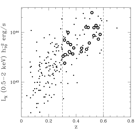
Figure 1.— X-ray luminosity as a function of redshift for the 160 square degree survey from Mullis et al. (2003). The large open points indicate the clusters for which HST imaging data were obtained.

2.1. Shape analysis

The first step in the weak lensing analysis is the detection of stars and galaxies, for which we use SExtractor (Bertin & Arnouts, 1996). The next important step is the unbiased measurement of the shapes of the faint background galaxies that will be used to quantify the lensing signal. To do so, we measure weighted quadrupole moments, defined as

$$I_{ij}=\int d^{2}{\mbox{{\it\boldmath$x$}}}x_{i}x_{j}W({\mbox{{\it\boldmath$x$}}})f({\mbox{{\it\boldmath$x$}}}),$$ (1)

where $W({\mbox{{\it\boldmath$x$}}})$ is a Gaussian with a dispersion $r_{g}$, which is matched to the size of the object (see Kaiser et al., 1995; Hoekstra et al., 1998, for more details). These quadrupole moments are combined to form the two-component polarization

$$e_{1}=\frac{I_{11}-I_{22}}{I_{11}+I_{22}},~{}{\rm and}~{}e_{2}=\frac{I_{12}}{I_{11}+I_{22}}.$$ (2)

However, we cannot simply use the observed polarizations, because they have been modified by a number of instrumental effects. Although the PSF of HST is small compared to ground based data, the shapes of the galaxies are nonetheless slightly circularized, lowering the amplitude of the observed lensing signal. Furthermore, the PSF is not round and the resulting anisotropy in the galaxy shapes needs to be undone. To do so, we use the well established method proposed by Kaiser et al. (1995), with the modifications provided in Luppino & Kaiser (1997) and Hoekstra et al. (1998, 2000).

2.2. Correction for CTE degradation

An issue that is relevant for ACS observations is the degradation of the charge transfer efficiency (CTE) with time. Over time, cosmic rays cause an increasing number of defects in the detector. During read-out, these defects can trap charges for a while. The delayed transfer of charge leads to a trail of electrons in the read-out direction, causing objects to appear elongated. The effect is strongest for faint objects, because brighter objects quickly fill the traps. Rhodes et al. (2007) provide a detailed discussion of CTE effects and their impact on weak lensing studies. Similar to Rhodes et al. (2007) we derive an empirical correction for CTE, but our adopted approach differs in a number of ways.

The presence of CTE in our data leads to a slight modification of our lensing analysis. First, we note that CTE affects only $e_{1}$ and that the change in shape occurs during the read-out stage. Hence the measured value for $e_{1}$ needs to be corrected for CTE before the correction for PSF anisotropy and circularization:

$$e_{1}=e_{1}^{\rm obs}-e_{1}^{\rm CTE},$$ (3)

where $e_{1}^{\rm CTE}$ is the predicted change in polarization given by the model derived in the Appendix. To derive our CTE model, we used observations of the star cluster NGC 104 as well as 100 exposures from the COSMOS survey (Scoville et al., 2007). The observations of a star cluster allow us to study the effect of CTE as a function of position, time and signal-to-noise ratio with high precision, because stars are intrinsically round after correction for PSF anisotropy. We find that the CTE effect increases linearly with time and distance from the read-out electronics. The amplitude of the effect is observed to be proportional to $\sqrt{S/N}$. We use 100 exposures from COSMOS to examine how the CTE effect depends on source size. We find a strong size dependence, with $e_{1}^{\rm CTE}\propto r_{g}^{-2}$ (where $r_{g}$ is the dispersion of the Gaussian weight function used to measure the quadrupole moments).

2.3. Correction for the PSF

Once the CTE effect has been subtracted for all objects (including stars), the lensing analysis proceeds as described in Hoekstra et al. (1998). Hence the next step is to correct both polarization components for PSF anisotropy. The ACS PSF is time dependent and therefore a different PSF model is required for each observation. An added complication is the fact that only a limited number of stars are observed in each image.

To estimate the spatial variation of the PSF anisotropy a number of procedures have been proposed (Rhodes et al., 2007; Schrabback et al., 2007, 2010). Here we opt for a simple approach, similar to the one used in Hoekstra et al. (1998).

Figure 2.— PSF reference model based on observations of NGC104. The sticks show the direction and amplitude (indicated by the length) of the polarization of the PSF. The PSF anisotropy is generally small, but can reach 4% at the edges of the field.

We use observations of the star cluster NGC104 to derive an adequate model for PSF anisotropy. These data were taken at the start of ACS operations (PID 9018), and therefore do not suffer from CTE effects. We model the PSF anisotropy by a third order polynomial in both $x$ and $y$. Such a model would not be well constrained by our galaxy cluster data, but it is thanks to the high number density of stars in NGC104. We select one of the models as our reference, because the PSF pattern varied only mildly from exposure to exposure. The resulting reference model is shown in Figure 2. The PSF anisotropy is fairly small, but can reach $\sim 4\%$ towards the edges of the field.

Most of the variation in the ACS PSF arises from focus changes, which are the result of changes in the telescope temperature as it orbits the Earth. We therefore expect that a scaled version of our model can capture much of the spatial variation: as the detector moves from one side of the focus to the other, the direction of PSF anisotropy changes by 90 degrees, which corresponds to a change of sign in the polarization. To account for additional low order changes, we also include a first order polynomial:

$$e_{i}^{\rm PSF}=\alpha e_{i}^{\rm NGC104}+a_{0}+a_{1}x+a_{2}y.$$ (4)

This simple model, with only 4 parameters, is used to characterize the PSF anisotropy for each individual galaxy cluster exposure. The number of stars in the galaxy cluster images ranges from 7 to 84, with a median of 20. To examine how well our approach works, we averaged the shapes of all the stars in our 25 galaxy cluster exposures. The ensemble averaged PSF polarization as a function of position is shown in Figure 3. The open points show the average PSF shapes before correction. More importantly, the filled points show the residuals in polarization after the best fit model for each galaxy cluster pointing has been subtracted. These results suggest our model is adequate for our weak lensing analysis.

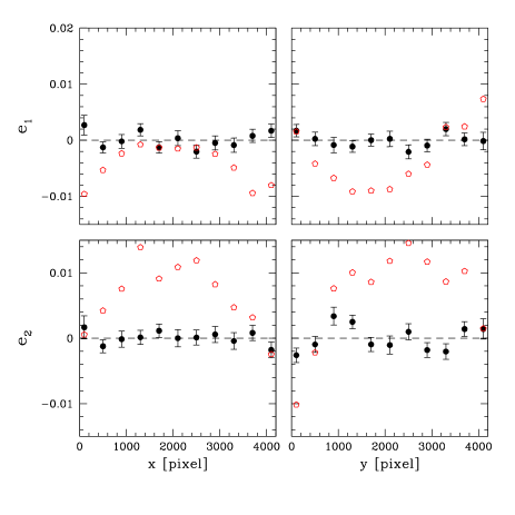
Figure 3.— The ensemble averaged PSF polarization $e_{1}$ and $e_{2}$ as a function of position using stars detected in our galaxy cluster exposures. The open circles show the PSF anisotropy before correction, whereas the solid points correspond to the residuals after applying the best fit PSF model to the stars.

2.4. Lensing signal

The corrected galaxy shapes are used to measure the weak lensing signal. A convenient way to quantify the lensing signal is by computing the azimuthally averaged tangential shear $\gamma_{T}$ as a function of radius from the cluster center (see §2.5 for our choice of the center). It can be related to the surface density through

$$\langle\gamma_{t}\rangle(r)=\frac{\bar{\Sigma}(<r)-\bar{\Sigma}(r)}{\Sigma_{\rm crit}}=\bar{\kappa}(<r)-\bar{\kappa}(r),$$ (5)

where $\bar{\Sigma}(<r)$ is the mean surface density within an aperture of radius $r$, and $\bar{\Sigma}(r)$ is the mean surface density on a circle of radius $r$. The convergence $\kappa$, or dimensionless surface density, is the ratio of the surface density and the critical surface density $\Sigma_{\rm crit}$, which is given by

$$\Sigma_{\rm crit}=\frac{c^{2}}{4\pi G}\frac{D_{s}}{D_{l}D_{ls}},$$ (6)

where $D_{l}$ is the angular diameter distance to the lens. $D_{s}$ and $D_{ls}$ are the angular diameter distances from the observer to the source and from the lens to the source, respectively. The parameter $\beta=\max[0,D_{ls}/D_{s}]$ is a measure of how the amplitude of the lensing signal depends on the redshifts of the source galaxies (where a value of 0 is assigned to sources with a redshift lower than that of the cluster).

One of the advantages of weak lensing is that the (projected) mass can be determined in a model-independent way. To derive accurate masses requires wide field imaging data, which we lack because of the small field of view of ACS. Instead we fit parametric models to the lensing signal.

The singular isothermal sphere (SIS) is a simple model to describe the cluster mass distribution. In this case the convergence and tangential shear are equal:

$$\kappa(r)=\gamma_{T}(r)=\frac{r_{E}}{2r},$$ (7)

where $r_{E}$ is the Einstein radius. In practice we do not observe the tangential shear directly, but we observe the reduced shear $g_{T}$ instead:

$$g_{T}=\frac{\gamma_{T}}{1-\kappa}.$$ (8)

We correct our model predictions for this effect. Under the assumption of isotropic orbits and spherical symmetry, the Einstein radius (in radian) can be expressed in terms of the line-of-sight velocity dispersion:

$$r_{E}=4\pi\left(\frac{\sigma}{c}\right)^{2}\beta.$$ (9)

We use this model when listing lensing inferred velocity dispersions in Table 2.

A more physically motivated model is the one proposed by Navarro et al. (1997) who provide a fitting function to the density profiles observed in numerical simulations of cold dark matter. We follow the conventions outlined in Hoekstra (2007), but use an updated relation between the virial mass $M_{\rm vir}$ and concentration $c$. Duffy et al. (2008) studied numerical simulations using the best fit parameters of the WMAP5 cosmology (Komatsu et al., 2009). The best fit $c(M_{\rm vir})$ is given by:

$$c=7.85\left({\frac{M_{\rm vir}}{2\times 10^{12}}}\right)^{-0.081}{(1+z)^{-0.71}}.$$ (10)

We use this relation when fitting the NFW model to the lensing signal. Rather than the virial mass, in Table 2 we list $M_{2500}$ which is the mass within a radius $r_{2500}$ where the mean mass density of the halo is 2500 times the critical density at the redshift of the cluster. We note that a different choice for the mass-concentration relation will change the inferred masses much. We found that the inferred values for $M_{2500}$ change by $5-10\%$ if we change the pre-factor in Equation 10 by $\pm 1$, which is much smaller than our statistical uncertainties. When comparing to ensemble averaged results from other studies, however, differences in the adopted mass-concentration relation may become a dominant source of uncertainty.

Finally, we note that the lensing signal is sensitive to all matter along the line-of-sight. As shown in Hoekstra (2001, 2003), the large-structure in the universe introduces cosmic noise, which increases the formal error in the mass estimate, compared to just the statistical uncertainty. The listed uncertainties in the weak lensing masses include this contribution.

2.5. Cluster center

We have to choose a position around which we measure the weak lensing signal as a function of radius. An offset between the adopted position and the ‘true’ center of the dark matter halo will lead to an underestimate of the cluster mass. Possible substructure in the cluster core complicates a simple definition of the cluster center, but it can also lead to biased mass estimates (e.g., Hoekstra et al., 2002). We expect our results to be less affected by substructure because the ACS data used here extend to larger radii than the WFPC2 observations discussed in Hoekstra et al. (2002).

The resulting bias depends on the detailed procedure that is used to to interpret the lensing signal. For instance, Hoekstra (2007) used wide field imaging data to measure the lensing signal out to large radii and to derive (almost) model-independent masses. This procedure minimizes the effect of centroiding errors because the large-scale signal is affected much less, compared to the signal on small scales. Unfortunately, the ACS field of view is relatively small, which prevents us from following the same approach and we fit a parameterized mass model to the lensing signal instead. To reduce the sensitivity of our results to centroiding errors and central substructure, we fit the NFW and SIS models to the tangential distortion at radii $200<r<750h_{70}^{-1}$kpc.

The advantage of restricting the analysis to larger scales is also evident from Figure 4, where we show the bias in mass as a function of centroid offset $r_{\rm off}$. The solid curve shows the results when fitting an NFW model to the signal within $200-750h^{-1}_{70}$ kpc, which is the range we use for the ACS data studied here.

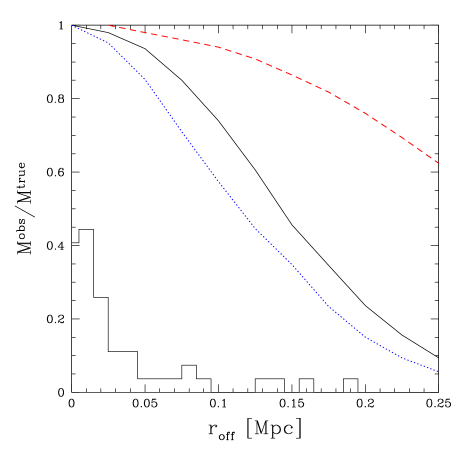
Figure 4.— Plot of the ratio of the inferred lensing mass and the true mass as a function of centroid offset. The lensing mass is obtained by fitting an NFW model to the shear at $200-750h^{-1}_{70}$ kpc (solid black curve) and $0.5-1.5h^{-1}_{70}$Mpc (dashed red curve). The blue dotted line corresponds to the bias if all data within $750h^{-1}_{70}$ kpc are used. The results presented here are for a cluster with a mass $M_{2500}=2\times 10^{14}h_{70}^{-1}\hbox{$\rm{M}_{\odot}$}$, but we note that the bias varies only by a few percent over the range of masses we consider here. The histogram indicates the frequency of offsets found for massive clusters from Bildfell et al. (2008).

Mullis et al. (2003) provide cluster positions based on the X-ray emission. For the clusters in our sample, the listed centroiding uncertainty depends on the X-ray luminosity (with smaller values for the more luminous systems). An alternative approach is to use the location of the brightest cluster galaxy (BCG). The resulting positions are listed in Table 1. In many cases a clear candidate can be identified (indicated by a value of $Q_{\rm BCG}$ of 1 or 2 in Table 1), but in a number of cases the choice is ambiguous (indicated by $Q_{\rm BCG}$ -1 or 0).

High quality X-ray data can be used to refine the centers, but such data are lacking for our sample. Even if such data were available, there can be a offset between the BCG and the peak in the X-ray emission (e.g., Bildfell et al., 2008). The distribution of offsets observed by Bildfell et al. (2008) for the massive clusters in the Canadian Cluster Comparison Project, are indicated by the histogram in Figure 4. It is clear that the offsets are typically less than 50 kpc, leading to biases less than 5%. The larger offsets are found for merging massive systems where the identification of the BCG is difficult. Such major mergers do not appear to be present in the sample of clusters studied here.

We compared the offset between the X-ray position and the adopted location of the BCG to the uncertainty listed in Mullis et al. (2003) and find fair agreement: most of the BCGs are located within the radius corresponding to the 90% confidence X-ray position error circle. Only for 4 low luminosity systems do we find an offset that is much larger. The positions of the BCGs can be determined more accurately, and we therefore adopt these as the cluster centers when listing our mass estimates.

2.6. Source galaxies

The lensing signal is largest for background galaxies at redshifts much larger than the cluster. We lack redshift information for our sources and instead we select a sample of faint (distant) galaxies with $24<F814W<26.5$, which also reduces contamination by cluster members which dominate the counts at bright magnitudes. Nonetheless, contamination by cluster members cannot be ignored because we lack color information. We note that adding a single color would not improve the situation significantly because the faint members span a wide range in color, unlike the bright members, almost all of which occupy a narrow red-sequence.

To account for contamination by cluster members we measure the number density of faint galaxies as a function of distance from the adopted cluster center and boost the signal by the inferred fraction of cluster members. The corrected tangential distortion for RXJ0847.1+3449 as a function of distance from the adopted cluster centre is shown in Figure 5a. The red line shows the best fit singular isothermal sphere model (fitted to radii $>25^{\prime\prime}$). If the observed signal is caused by gravitational lensing, the signal should vanish if the source galaxies are rotated by 45 degrees. Figure 5b shows the results of this test, which are indeed consistent with no signal.

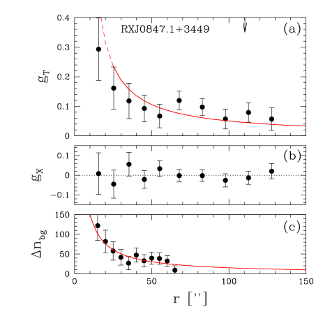
Figure 5.— panel a: Tangential distortion as a function of radius for RXJ0847.1+3449. The measurements have been corrected for contamination by faint cluster member using the best fit model to the excess counts shown in panel c. The best fit SIS model based on a fit to the measurements at $r>25$ arcseconds is indicated by the drawn line. The arrow indicates a radius of $0.5h^{-1}$Mpc. panel b: The signal when the sources are rotated by 45 degrees. In this case the signal should vanish if the measurements shown in panel a are due to gravitational lensing. panel c: Excess counts of galaxies with $24<F814W<26.5$ as compared to the mean counts based on 100 frames from the COSMOS survey. The expected background counts are $\sim 61$ arcmin^-2. The drawn line is the best fit $1/r$ model, which is used to correct the measurements of the tangential distortion.

The lower panel in Figure 5 shows the excess counts $\Delta n_{\rm bg}$ as a function of radius for the cluster RXJ0847.1+3449 ($z=0.56$). To determine the background count levels we used the 100 COSMOS pointings that were used to measure the size-dependence of CTE. We measure the excess counts for each cluster individually, because the sample spans a fair range in redshift and mass.

This cluster shows a signicant excess of faint galaxies over the background number density of $\sim 61$ arcmin^-2. We assume that these faint cluster members are oriented randomly and thus simply dillute the lensing signal. To quantify the overdensity of faint members we adopt $\Delta n_{\rm bg}\propto r^{-1}$ and determine the best fit normalization for each cluster separately (indicated by the drawn line in Figure 5c. This simple model is used to correct the observed tangential distortion for contamination by cluster members. We find that this correction leads to an average increase in the best fit Einstein radius of $\sim 20\%$. The uncertainty in the amplitude of the contamination is included in our quoted measurement errors (which are increased by less than 5%).

The conversion of the lensing signal into an estimate for the mass of the cluster requires knowledge of the redshift distribution of the source galaxies. These are too faint to be included in spectroscopic redshift surveys or even from ground based photometric redshift surveys (e.g., Wolf et al., 2004; Ilbert et al., 2006). Instead we use the photometric redshift distributions determined from the Hubble Deep Fields (Fernández-Soto et al., 1999). For the range in apparant magnitudes used in the lensing analysis, the resulting average value for $\langle\beta\rangle$ and the variance $\langle\beta^{2}\rangle$ are listed in Table 1. As discussed in Hoekstra et al. (2000) the latter quantity is needed to account for the fact that we measure the reduced shear. We estimate the uncertainty in $\beta$ by considering the variation between the two HDFs. As the average source redshift is much higher than the cluster redshifts, the resulting relative uncertainties are small: $\sim 2\%$ at $z=0.3$, increasing to $\sim 5\%$ at $z=0.6$, much smaller than our statistical errors.

Table 2Measurements of cluster properties

name	$r_{E}$	$\sigma$	$r_{2500}$	$M_{2500}$	$N_{2500}$
	[”]	[km/s]	[$h_{70}^{-1}$Mpc]	[$h_{70}^{-1}10^{13}$M⊙]
RXJ$0056.9-2740$	$5.4\pm 1.5$	$678^{+88}_{-101}$	0.270	$5.2^{+4.2}_{-3.0}$	$13\pm 4$
RXJ$0110.3+1938$	$5.8\pm 1.3$	$577^{+62}_{-69}$	0.293	$5.0^{+3.4}_{-2.6}$	$4\pm 2$
RXJ$0154.2-5937$	$3.6\pm 1.4$	$474^{+83}_{-101}$	0.218	$2.2^{+2.6}_{-1.4}$	$1\pm 1$
RXJ$0522.2-3625$	$6.8\pm 1.3$	$710^{+66}_{-73}$	0.313	$7.2^{+4.2}_{-3.1}$	$7\pm 3$
RXJ$0826.1+2625$	$2.4\pm 1.8$	$384^{+124}_{-192}$	0.157	$0.8^{+2.1}_{-2.1}$	$2\pm 1$
RXJ$0841.1+6422$	$7.5\pm 1.3$	$668^{+55}_{-59}$	0.354	$9.0^{+3.9}_{-3.5}$	$15\pm 4$
RXJ$0847.1+3449$	$10.3\pm 1.7$	$937^{+74}_{-80}$	0.452	$24.2^{+8.9}_{-7.6}$	$21\pm 5$
RXJ$0910.6+4248$	$3.5\pm 1.7$	$551^{+121}_{-157}$	0.246	$4.0^{+4.7}_{-2.9}$	$3\pm 2$
RXJ$0921.2+4528$	$2.1\pm 1.5$	$344^{+108}_{-164}$	0.180	$1.2^{+1.8}_{-1.2}$	$5\pm 2$
RXJ$0926.6+1242$	$8.9\pm 1.5$	$822^{+65}_{-70}$	0.407	$16.2^{+6.0}_{-5.1}$	$11\pm 4$
RXJ$0957.8+6534$	$4.5\pm 1.4$	$605^{+89}_{-105}$	0.257	$4.3^{+3.2}_{-2.6}$	$3\pm 2$
RXJ$1015.1+4931$	$6.0\pm 1.4$	$618^{+70}_{-79}$	0.296	$5.6^{+3.4}_{-2.9}$	$3\pm 2$
RXJ$1117.2+1744$	$1.9\pm 1.6$	$331^{+114}_{-185}$	0.252	$3.1^{+3.2}_{-2.1}$	$6\pm 3$
RXJ$1117.4+0743$	$5.5\pm 1.4$	$640^{+76}_{-86}$	0.280	$5.2^{+3.4}_{-2.8}$	$13\pm 4$
RXJ$1123.1+1409$	$5.8\pm 1.4$	$588^{+69}_{-78}$	0.271	$4.0^{+3.8}_{-2.6}$	$9\pm 3$
RXJ$1354.2-0221$	$9.6\pm 1.4$	$895^{+64}_{-69}$	0.428	$20.2^{+6.4}_{-5.6}$	$23\pm 5$
RXJ$1524.6+0957$	$4.3\pm 1.3$	$585^{+84}_{-98}$	0.336	$9.5^{+4.4}_{-3.8}$	$14\pm 4$
RXJ$1540.8+1445$	$4.0\pm 1.4$	$530^{+83}_{-99}$	0.279	$4.9^{+3.7}_{-2.5}$	$13\pm 4$
RXJ$1642.6+3935$	$2.2\pm 1.5$	$371^{+107}_{-156}$	0.239	$2.8^{+2.8}_{-1.8}$	$5\pm 2$
RXJ$2059.9-4245$	$4.4\pm 1.3$	$508^{+71}_{-82}$	0.280	$4.4^{+3.3}_{-2.4}$	$6\pm 3$
RXJ$2108.8-0516$	$3.4\pm 1.4$	$442^{+81}_{-100}$	0.210	$1.8^{+2.2}_{-1.4}$	$5\pm 2$
RXJ$2139.9-4305$	$5.2\pm 1.4$	$572^{+73}_{-84}$	0.292	$5.3^{+3.7}_{-2.6}$	$9\pm 3$
RXJ$2146.0+0423$	$8.5\pm 1.4$	$830^{+67}_{-73}$	0.436	$21.0^{+6.7}_{-5.7}$	$14\pm 4$
RXJ$2202.7-1902$	$1.5\pm 1.4$	$319^{+127}_{-252}$	0.152	$0.8^{+2.0}_{-0.8}$	$2\pm 1$
RXJ$2328.8+1453$	$4.9\pm 1.4$	$612^{+81}_{-93}$	0.254	$4.0^{+3.7}_{-2.6}$	$6\pm 3$

3. Results

As discussed above, we consider two often used parametric models for the cluster mass distribution. We fit these to the observed lensing signal at $200-750h_{70}^{-1}$kpc from the cluster center. The resulting Einstein radii and velocity dispersions are listed in Table 2. We also list the best-fit value for $M_{2500}$ inferred from the NFW model fit to the signal, where we use the mass-concentration relation given by Eqn. 10. For reference we also list the corresponding value for $r_{2500}$ from the NFW fit.

We use this radius to compute $N_{2500}$, the excess number of galaxies with a rest-frame $B$-band luminosity $-22<M_{B}<-18.5$ within $r_{2500}$ (we assume passive evolution when computing the rest-frame $B$-band luminosity). Recent studies of the cluster richness consider only galaxies on the red-sequence, because of the higher contrast, which improves the signal-to-noise ratio of the measurement. Unfortunately we lack color information, and we compute the total excess of galaxies. The background count levels were determined using the COSMOS pointings that were used to measure the size-dependence of CTE.

Figure 6a shows the resulting lensing mass as a function of the restframe X-ray luminosity in the $0.1-2.4$ keV band. The luminosities and masses have been scaled to redshift zero assuming self-similar evolution with respect to the critical density (e.g., Kaiser, 1986; Bryan & Norman, 1998), where

$$E(z)=\frac{H(z)}{H_{0}}=\sqrt{\Omega_{m}(1+z)^{3}+\Omega_{\Lambda}}$$ (11)

for flat cosmologies. The solid points indicate the clusters from the sample studied here. The clusters from the 160SD survey for which X-ray temperatures have been determined (see §3.1) are indicated by blue points. To extend the range in X-ray luminosity we also show measurements for the massive clusters that were studied in Hoekstra (2007). We note, that Hoekstra (2007) used bolometric X-ray luminosities from Horner (2001), whereas here we use the restframe luminosities in the $0.1-2.4$ keV band (which are a factor $\sim 4$ smaller). We use the mass estimates from Mahdavi et al. (2008) which used new photometric redshift distributions, which were based on much larger data sets (Ilbert et al., 2006).

The agreement in lensing masses is good in the regions where the two samples overlap. However, the scatter in the mass-luminosity relation is substantial (both for the clusters studied here as well as the more massive clusters). We examined whether some of the scatter could be due to the uncertainty in the position of the cluster center, but find no difference when comparing results for clusters with different levels of confidence in the identification of the BCG (see $Q_{\rm BCG}$ in Table 1. It is worth noting, however, that we do not find any massive clusters $(>10^{14}M_{\odot})$ that are X-ray faint (i.e., $L_{X}<10^{44}$ erg/s), implying that the dispersion in the $M-L_{X}$ relation is relatively well-behaved.

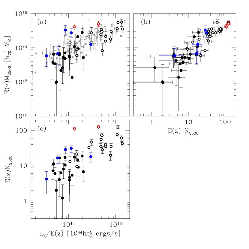
Figure 6.— panel a: Plot of $M_{2500}$ as a function of X-ray luminosity. To account for the range in redshift of the clusters, the mass and luminosity have been rescaled using the corresponding value for $E(z)$ under the assumption of self-similar evolution. The solid points are the clusters from the sample studied here. The solid blue points are the clusters from the 160SD survey for which X-ray temperatures have been determined (see §3.1). The open points correspond to the more massive clusters studied in Hoekstra (2007). The open red points indicate the well-known strong lensing clusters A370 and CL0024+16. For comparison the small grey points show the X-ray derived masses from Reiprich & Böhringer (2002), converted to $M_{2500}$; panel b: Plot of $M_{2500}$ as a function of $N_{2500}$, the excess of galaxies with restframe $-22<M_{B}<-18.5$ within $r_{2500}$; panel c: Plot of $N_{2500}$ as a function of X-ray luminosity.

Reiprich & Böhringer (2002) studied a sample of 63 X-ray bright clusters and derived masses under the assumption of hydrostatic equilibrium. This sample of clusters spans a similar range in $L_{X}$ as our combined sample. We converted their measurements for $M_{500}$ to $M_{2500}$ using the mass-concentration relation given by Eqn. 10 and show the results in Figure 6 (small grey points). The agreement with our findings is very good. A more quantitative comparison is presented in §3.3.

Yee & Ellingson (2003) have shown that there is a good relation between the cluster richness and the mass (and various proxies) for massive clusters. Our study extends to lower masses and as is shown in Figures 6b and c $N_{2500}$ correlates well with both the X-ray luminosity and lensing mass. Similar results have been obtained using SDSS cluster samples (e.g., Rykoff et al., 2008b; Johnston et al., 2007). We assumed that $N_{2500}$ scales as the mass $M_{2500}$, which is a reasonable assumption if the galaxies trace the density profile. This choice, however, does not affect our conclusions.

The results agree well in the regions where the two samples overlap. The correlation between $N_{2500}$ and $M_{2500}$ is tighter than that of $N_{2500}$ and $L_{X}$. The former is less sensitive to the projections along the line-of-sight (either substructures or an overall elongation of the cluster), because both the galaxy counts and the lensing mass are derived from projected measurements. The X-ray results provide a different probe of the distribution of baryons, which is expected to lead to additional scatter. Furthermore, some of the scatter may be caused by unknown contributions by AGNs. The importance of AGN can be evaluated using a combination of deeper, high spatial resolution $(\lesssim 5^{\prime\prime})$ X-ray and radio imaging. Such X-ray observations would also provide estimates for the temperature of the X-ray gas (which is a better measure of the cluster mass). Unfortunately, such data exist for only five of the low-mass clusters. For these, X-ray temperatures have been derived, which are listed Table 3. For the massive clusters we use the values from Horner (2001) that were used in Hoekstra (2007). We note that all clusters follow a tight $L_{x}-T_{x}$ relation.

3.1. Comparison with X-ray temperature

Figure 7 shows the resulting plot of $M_{2500}$ as a function of X-ray temperature. RXJ$1117.4+0743$ and RXJ$1524.6+0957$ lie on the tight relation defined by the bulk of the clusters. The measurements from Reiprich & Böhringer (2002) also follow this relation (light grey points). However, RXJ$0847.1+3449$ and RXJ$1354.2-0221$ appear to be more massive than might be expected based on $T_{X}$. They appear to lie on a parallel relation, along with some of the clusters from Hoekstra (2007). The latter clusters are CL0024+16 and A370, which are well known strong lensing clusters (indicated in red in Figures 6 and 7). These clusters were observed because of their strong lensing properties and included in the search for archival CFHT data carried out by Hoekstra (2007).

Interestingly, all four clusters are outliers on both the $M_{2500}$-$L_{x}$ and $N_{2500}-L_{x}$ relations presented in Figure 6, but follow the mass-richness relation. This is consistent with the presence of (sub)structures along the line-of-sight boosting both $M_{2500}$ and $N_{2500}$: the projection of two mass concentrations (along the line-of-sight) would increase the richness and the weak lensing mass approximately linearly. The inferred X-ray temperature on the other hand will be close to that of the more massive system, whereas the X-ray luminosity will be much lower than expected, because it is proportional to the square of the electron density. We note that both RXJ$0847.1+3449$ and RXJ$1354.2-0221$ show evidence of strong lensing.

Table 3X-ray temperatures

name	$kT_{X}$ [keV]	ref.
RXJ$0110.3+1938$	$1.46^{+0.19}_{-0.15}$	1
RXJ$0847.1+3449$	$3.62^{+0.58}_{-0.51}$	2
RXJ$1117.4+0743$	$3.3^{+0.42}_{-0.36}$	3
RXJ$1354.2-0221$	$3.66^{+0.6}_{-0.5}$	2
RXJ$1524.6+0957$	$5.1\pm 0.36$	4

Interestingly, the X-ray image of RXJ$0847.1+3449$ in Lumb et al. (2004) shows evidence for a nearby cluster candidate. The case is less clear for RXJ$1354.2-0221$, but the X-ray image shows a complex morphology. Unfortunately we lack the dynamical data to confirm whether RXJ$0847.1+3449$ and RXJ$1354.2-0221$ are projected systems. The cluster RXJ$1117.4+0743$ was studied in detail by Carrasco et al. (2007), who find that this cluster is also a projection of two structures. For the main component Carrasco et al. (2007) infer a galaxy velocity dispersion of $592\pm 82$ km/s, whereas the second structure is less massive with $\sigma_{v}=391\pm 85$ km/s. Based on our lensing analysis we obtained a velocity dispersion of $639^{+76}_{-86}$ km/s, in good agreement with the dynamical results for the main cluster. Carrasco et al. (2007) also performed a weak lensing analysis based on ground based imaging data and obtained a velocity dispersion of $\sigma=778\pm 89$ km/s (where we took the average of their results for the $g^{\prime}$ and $r^{\prime}$ band), implying a mass 50% larger than our estimate. We are not able identify an obvious cause for this difference, but note that PSF-related systematics have a larger impact on ground based results.

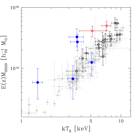
Figure 7.— Plot of $M_{2500}$ as a function of X-ray temperature. To account for the range in redshift of the clusters, the mass has been rescaled using the corresponding value for $E(z)$ under the assumption of self-similar evolution. The solid blue points are the clusters from the sample studied here. The open points correspond to the more massive clusters studied in H07, whereas the small grey points show the results from Reiprich & Böhringer (2002). The well-known strong lenses A370 and CL0024+16 are indicated as red open points.

3.2. The $M_{2500}-L_{X}$ scaling relation

In this section we examine the correlation between $M_{2500}$ and the X-ray luminosity, in particular the normalization and the power law slope. We fit a power law model to the combined sample to maximize the leverage in X-ray luminosity

$$E(z)M_{2500}=M_{x}\left(\frac{L_{x}/E(z)}{2\times 10^{44}{\rm erg/s}}\right)^{\alpha}.$$ (12)

If we naively fit this model to the measurements we find that the value for $\chi^{2}$ of the best fit is too high ($\chi^{2}=106$ with 43 degrees of freedom). This indicates that there is intrinsic scatter in the relation, which is also apparent from Figure 6. We need to account for the intrinsic scatter in the fitting procedure, because ignoring it will generally bias the best fit parameters. We fit the model to our measurements, which have errors that follow a normal distribution. The intrinsic scatter, however, can be described by a log-normal distribution (see e.g., Fig. 13 in Vikhlinin et al., 2009a). We will assume that the intrinsic scatter can be approximated with a normal distribution with a dispersion $\sigma_{Q}\approx\ln(10)Q\log Q$ (we use the log with base 10).

To fit the $M_{2500}-L_{X}$ relation we follow a maximum likelihood approach. For a model $f$ with parameters ${\bf a}$, the predicted values are $y_{i}=f(x_{i};{\bf a})$. The uncertainties in $x_{i}$ and $y_{i}$ are given by $\sigma_{x,i}$ and $\sigma_{y,i}$. If we assume a Gaussian intrinsic scatter $\sigma_{Q,i}$ in the $y_{i}$ coordinate, the likelihood ${\cal L}$ is given by

$${\cal L}=\prod_{i=1}^{n}\frac{1}{\sqrt{2\pi}w_{i}}\exp\left[-\frac{[y_{i}-f(x_{i};{\bf a})]^{2}}{2w_{i}^{2}}\right],$$ (13)

where $w_{i}$ accounts for the scatter:

$$w_{i}^{2}=\left[{\frac{df}{dx}(x_{i})}\right]^{2}\sigma_{x,i}^{2}+\sigma_{y,i}^{2}+\sigma_{Q,i}^{2}.$$ (14)

If we consider the logarithm of the likelihood it becomes clear why including the intrinsic scatter differs from standard least squares minimization:

$$-2\ln{\cal L}=2\sum_{i=1}^{n}\ln w_{i}+\sum_{i=1}^{n}\left(\frac{y_{i}-f(x_{i};a_{j})}{w_{i}}\right)^{2}+C,$$ (15)

where the second term corresponds to the usual $\chi^{2}$. For a linear relation with no intrinsic scatter, the first term is a constant for a given data set and the likelihood is maximimized by minimizing $\chi^{2}$. However, if intrinsic scatter is included as a free parameter, the first term acts as a penalty function, and cannot be ignored.

The presence of intrinsic scatter also exacerbates the Malmquist bias for a flux limited sample, such as the 160SD survey. As a result the average flux of the observed sample of clusters is biased high compared to the mean of the parent population (in particular near the flux limit of the survey). To account for Malmquist bias we follow the procedure outlined in Appendix A.2 of Vikhlinin et al. (2009a) and correct the X-ray luminosities before fitting the $M_{2500}-L_{X}$ relation. We find that the correction for Malmquist bias is relatively modest, increasing the normalisation $M_{X}$ by $\sim 5\%$ and reducing the slope $\alpha$ by $\sim 5\%$.

We find an intrinsic scatter of $\sigma_{\log L_{X}|M}=0.23^{+0.10}_{-0.04}$ (or a relative error of $\sim 70\%$), in good agreement with other studies. Reiprich & Böhringer (2002) list a somewhat larger scatter of $\sigma_{\log L_{X}|M}=0.29$ for the HIFLUGCS sample, whereas Vikhlinin et al. (2009a) and Mantz et al. (2010a) find $\sigma_{\log L_{X}|M}=0.17\pm 0.02$ and $0.18\pm 0.02$, respectively. Our results also agree well with Stanek et al. (2006) who find $\sigma_{\log M|L_{X}}=0.19\pm 0.03$, which is in good agreement with our value of $0.17^{+0.04}_{-0.03}$.

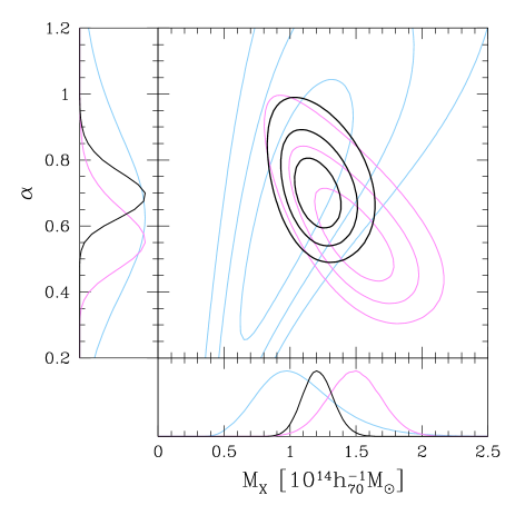
Figure 8.— Likelihood contours for the slope of the $M_{2500}-L_{X}$ relation and the mass of a cluster with a luminosity of $L_{X}=2\times 10^{44}h_{70}^{-2}$ ergs/s. The contours indicate the 68.3%, 95.4% and 99.7% confidence limits on two parameters jointly. The side panels show the probability density distributions for each parameter (while marginalising over the other). The black curves correspond to the constraints determined from the combined sample of clusters, whereas the cyan and pink curves correspond to the low mass and high mass samples, respectively.

The likelihood contours for the power law slope $\alpha$ of the $M_{2500}-L_{X}$ relation and the mass $M_{2500}$ of a cluster with a luminosity of $L_{X}=2\times 10^{44}h_{70}^{-2}$erg/s are shown in Figure 8. For the combined sample of clusters we find a best fit slope of $\alpha=0.68\pm 0.07$ and a normalization $M_{X}=(1.2\pm 0.12)\times 10^{14}h_{70}^{-1}\hbox{$\rm{M}_{\odot}$}$. The inferred slope is consistent with the value of $\frac{3}{4}$ expected for self-similar evolution (Kaiser, 1986).

It is also interesting to compare the constraints from both sub-samples separately. The best fit slope for the clusters studied in Hoekstra (2007) is $\alpha=0.55^{+0.10}_{-0.09}$ with a normalization of $M_{X}=(1.5\pm 0.2)\times 10^{14}h_{70}^{-1}\hbox{$\rm{M}_{\odot}$}$ (indicated by the pink contours). The blue contours in Figure 8 indicate the constraints for the HST sample studied here. The parameters are not well constrained, with best fit values $\alpha=0.63\pm 0.24$ and a normalization $M_{X}=(1.0\pm 0.24\times 10^{14}h_{70}^{-1}\hbox{$\rm{M}_{\odot}$}$.

The difference in the constraints from the (extended) Hoekstra (2007) sample and the 160SD systems may hint at a deviation from a single power law relation. As discussed in §2.5, however, the uncertainty in the position of the cluster center leads to an underestimate of the cluster mass, as does the presence of substructure. The Hoekstra (2007) results are much less sensitive to these problems. To quantify this, we combine the Hoekstra (2007) results with the 160SD clusters with $Q_{\rm BCG}=2$ (12 systems) and the ones with $Q_{\rm BCG}<2$ (13 systems). For the former we find $M_{X}=(1.30\pm 0.15)\times 10^{14}h_{70}^{-1}\hbox{$\rm{M}_{\odot}$}$ and $\alpha=0.63\pm 0.08$, whereas requiring $Q_{\rm BCG}<2$ yields $M_{X}=(1.19\pm 0.14)\times 10^{14}h_{70}^{-1}\hbox{$\rm{M}_{\odot}$}$ and $\alpha=0.68\pm 0.08$. This comparison suggests that our normalisation may be biased low by as much as $\sim 10\%$.

3.3. Comparison with X-ray samples

The relation between the X-ray luminosity and cluster mass has been studied extensively. In this section we compare our measurements to a number of recent results, which are shown in Figure 9. Where needed, the X-ray luminosities are converted to the $0.1-2.4$ keV band and Eqn. 10 has been used to convert masses to $M_{2500}$ and adjust the slopes (because the relation between $M_{2500}$ and $M_{200}$ (or $M_{500}$) is a power law with a slope less than 1.).

Reiprich & Böhringer (2002) studied a sample of 63 clusters, with masses derived under the assumption of hydrostatic equilibrium. Their BCES bisector results for the flux-limited sample yields $\alpha=0.60\pm 0.05$ and $M_{x}=(1.3\pm 0.09)\times 10^{14}\hbox{$\rm{M}_{\odot}$}$ are indicated by the blue triangle in Fig. 9. Stanek et al. (2006), however, have argued that these results suffer from Malmquist bias. Instead they compared the X-ray number counts to the mass function in $\Lambda$CDM cosmologies and derived $\alpha=0.54\pm 0.02$ and a high normalization of $M_{X}=(2.1\pm 0.1)\times 10^{14}\hbox{$\rm{M}_{\odot}$}$. This result, however depends strongly on the adopted value for $\sigma_{8}$, and combination with the WMAP3 data (Spergel et al., 2007) lowers the normalization to $M_{X}=(1.56\pm 0.08)\times 10^{14}\hbox{$\rm{M}_{\odot}$}$ (open pink triangle in Fig. 9). Vikhlinin et al. (2009a) studied a sample of $z\sim 0.05$ and $z\sim 0.5$ clusters that were observed with Chandra. Their results with $\alpha=0.55\pm 0.05$ and $M_{x}=(1.43\pm 0.08)\times 10^{14}\hbox{$\rm{M}_{\odot}$}$ are indicated by the open orange square. Another recent study was presented by Mantz et al. (2010a) who found a fairly steep slope of $\alpha=0.70\pm 0.04$ and $M_{x}=(1.42\pm 0.28)\times 10^{14}\hbox{$\rm{M}_{\odot}$}$ (purple square).

The constraints from these studies are largely driven by X-ray luminous clusters (this is particularly true for the results of Vikhlinin et al. (2009a) and Mantz et al. (2010a)). If the slope of the $M_{2500}-L_{X}$ varies with $L_{X}$, then it is more appropriate to compare these studies to the results from the sample studied in Hoekstra (2007), for which the agreement is indeed very good. When combined with the results from the 160SD survey, the resulting scaling relation has a lower normalisation and steeper slope. To examine whether this could be caused by a change in slope, it is interesting to compare to measurements at lower luminosities.

At the low X-ray luminosity end, Leauthaud et al. (2010) studied X-ray groups using COSMOS. Because of the small area surveyed, the groups are less luminous than the sample of clusters from the 160SD survey studied here. Nonetheless it is interesting to extrapolate their results for comparison. Leauthaud et al. (2010) use the mass-concentration relation from Zhao et al. (2009). We refit the 160SD sample using this relation and find that the average $M_{2500}$ is unchanged, but that $M_{200}$ is increased by 24%. We account for this when converting the measurements from Leauthaud et al. (2010), and find that they imply $M_{x}=(1.4\pm 0.3)\times 10^{14}\hbox{$\rm{M}_{\odot}$}$ and a slope $\alpha=0.61\pm 0.13$ (indicated by the open green circle in Fig. 9), in fair agreement with our results. We also note that this highlights the difficulty in comparing results, especially when the analyses differ in detail. This is particularly relevant for the comparison with SDSS results in the following section.

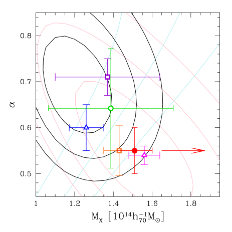
Figure 9.— Comparison of the slope of the $M_{2500}-L_{X}$ relation and the mass of a cluster with a luminosity of $L_{X}=2\times 10^{44}h_{70}^{-2}$ ergs/s. The contours are the same as in Figure 8. The blue triangle indicates the results from Reiprich & Böhringer (2002). The result from Stanek et al. (2006) is indicated by the open pink triangle. We also show constraints from two recent studies of massive clusters by Vikhlinin et al. (2009a) (orange square) and Mantz et al. (2010a) (purple square). The results from a study of X-ray groups in COSMOS by Leauthaud et al. (2010) are indicated by the green circle. Note that the accuracy of the comparison is limited, because of differences in the mass-concentration relation. The results from Rykoff et al. (2008a) based on SDSS data are indicated by the red point. The arrow indicates the possible shift in mass because of a bias in the source redshift distribution.

3.4. Comparison with SDSS

Rykoff et al. (2008a) measured the scaling relation between $L_{X}$ and $M_{200}$ for a large sample of optically selected clusters found in the Sloan Digital Sky Survey (Koester et al., 2007). This allowed them to extend the study of the $M-L_{X}$ relation to much lower luminosities, compared to most of the measurements presented in the previous section. The clusters were binned in richness and for each bin, the mean X-ray luminosity and weak lensing mass were determined. In the lensing analysis, described in (Johnston et al., 2007), both the mass and concentration are fit as free parameters. The resulting values for $c$ agree well with the relation presented in Duffy et al. (2008). Upon conversion to $M_{2500}$ we find that the measurements from Rykoff et al. (2008a) correspond to $M_{X}=(1.5\pm 0.1)\times 10^{14}h_{70}^{-1}\hbox{$\rm{M}_{\odot}$}$ and $\alpha=0.55\pm 0.04$. This result is indicated in Figure 9 by the red point.

Mandelbaum et al. (2008b) have pointed out that the weak lensing masses determined by Johnston et al. (2007) may be too low (by as much as $\sim 24\%$), because of a bias in the source redshift distribution (also see Leauthaud et al., 2010). The red arrow indicates the shift in normalization if the bias pointed out by Mandelbaum et al. (2008b) is correct. In that case the results from Rykoff et al. (2008a) disagree with all other measurements.

Rykoff et al. (2008a) find a shallower slope and higher mass, which appears to be inconsistent with our results. As discussed above, uncertainties in the adopted cluster centers may lead us to underestimate our normalisation by as much as $\sim 10\%$, which is not sufficient to remove the difference. Johnston et al. (2007) model the centroiding uncertainty using results from mock catalogs. However, if the model overestimates the offsets the resulting masses will be biased high and Mandelbaum et al. (2008a) argue that this may indeed be the case.

Another possible explanation for the large normalisation of Rykoff et al. (2008a) is that their results are expected to be biased towards a lower $L_{X}$ at a given lensing mass. The reason for this was already alluded to in §3.1, namely that some clusters appear X-ray underluminous and have low X-ray temperatures, given their high masses. These clusters, however do follow the tight mass-richness relation. Rykoff et al. (2008a) bin their clusters in richness and analyse stacked X-ray and lensing data. The fact that $N_{2500}$ and $M_{2500}$ are strongly correlated, then leads to a larger mean mass at a given X-ray luminosity.

The presence of substructure in the cluster (as well as filaments), will boost both the lensing and richness estimates relative to the X-ray luminosity. Such structures are numerous at the low mass end: it is rare to find an alignment of rich clusters, because they are rare, whereas an alignment of groups should be more frequent. Hence, the bias is likely to be mass dependent, increasing the masses of low X-ray luminosity systems by a larger fraction, compared to X-ray luminous clusters. The consequence is a flatter slope of the $M-L_{X}$ relation.

Comparison with numerical simulations can help clarify the amplitudes of the various biases listed above. However, the argument presented above highlights the danger of stacking samples of clusters when parameters are correlated. Identifying and quantifying such correlation requires well-characterized (both in selection and data coverage) and large samples of clusters. The 160SD clusters provide an excellent starting point, but increasing the number of cluster in this mass range with high quality X-ray data is of great importance to better constrain the scaling relations and to help interpret the results from stacked samples of clusters.

4. Conclusions

To extend the observed scaling relation between cluster mass and X-ray luminosity towards lower $L_{X}$, we have determined the masses of a sample of 25 clusters of galaxies drawn from the 160 square degree ROSAT survey (Vikhlinin et al., 1998). The clusters have redshifts $0.3<z<0.6$, and the X-ray luminosities range from $2\times 10^{43}$ to $2\times 10^{44}$ erg/s. The masses were determined based on a weak lensing analysis of images in the $F814W$ filter obtained using the ACS on the HST.

To measure the mass we assume that the brightest cluster galaxy indicates the center of the cluster. In most cases this leads to an unambiguous identification, but in a number of cases the choice of center is less clear. Nonetheless, we have verified that our choice of center does not affect the results for the inferred scaling relations.

To correctly interpret the weak lensing data, we derived an accurate emperical correction for the effects of CTE on the shapes of faint galaxies. We detect a significant lensing signal around most of the clusters. To increase the range in cluster properties, we extend the sample with massive clusters studied by Hoekstra (2007). The lensing masses agree well where the two samples overlap in $L_{X}$.

The inferred lensing masses correlate well with the overdensity of galaxies (i.e., cluster richness). The relation between mass and X-ray luminosity has significant intrinsic scatter. Under the assumption it follows a log-normal distribution we find a scatter of $\sigma_{\log L_{X}|M}=0.23^{+0.10}_{-0.04}$, which is in good agreement with other studies. We fit a power law relation between $M_{2500}$ and $L_{X}$ and find a best fit slope of $\alpha=0.68\pm 0.07$ and a normalisation (for $L_{X}=2\times 10^{44}h_{70}^{-2}$ erg/s) of $M_{X}=(1.2\pm 0.12)\times h_{70}^{-1}10^{14}\hbox{$\rm{M}_{\odot}$}$. Comparison with other studies is complicated by the fact that the conversion of the masses depends on the assumed mass-concentration relation. We find that the results for the sample of massive clusters from Hoekstra (2007) agrees well with a number of recent studies. The combination with clusters from the 160SD survey lowers the normalisation, which could be caused by a steepening of the $M-L_{X}$ relation. However, a study of low mass systems by Rykoff et al. (2008a) finds a higher normalisation.

Uncertainties in the position of the cluster center, as well as deviations from the adopted NFW profile (e.g., substructures) may bias our masses low, but we estimate this to be less than 10%, which cannot explain the difference with Rykoff et al. (2008a). On the other hand, structures along the line-of-sight, which also may simply reflect the fact that clusters themselves are highly elongated, will lead to a higher normalisation for the study by Rykoff et al. (2008a). They binned clusters discovered in the SDSS by richness and measured their ensemble averaged X-ray luminosity and lensing mass. In this case the tight correlation between lensing mass and richness results in a low average $L_{X}$ at a given mass. Furthermore, the relative importance of substructures and projections is mass dependent, preferentially affecting low mass systems. Consequently, both the slope and the normalization of the $M-L_{X}$ relation are affected.

To investigate the importance of the various biases, larger samples of low mass clusters need to be observed. Better X-ray observations provide a good starting point to extend the mass range over which scaling relations are determined and to improve the interpretation of ensemble averaged samples of clusters.

Appendix A Measurement of CTE effects

In this appendix we present the results of our study of the effect of CTE on shape measurements. Similar to other studies (e.g., Massey et al., 2007; Rhodes et al., 2007) we derive an empirical correction, although our actual implementation differs from these previous works in a number of ways.

The CTE problem occurs during readout, and therefore the correction should be applied before the correction for PSF anisotropy. Ideally one would like to correct the images before shape measurements are done (Massey et al., 2010), but for our purposes such a sophisticated approach is less important. Instead we will quantify the change in $e_{1}$ (this is the polarization component that quantifies the elongation along the $x-$ and $y-$ direction). We note that our measurements are done on images after they have been corrected for camera distortion.

Massey et al. (2007) measured the effect of CTE by determining the mean galaxy ellipticity as a function of distance from the readout electronics. We cannot do so for a number of reasons. First, we have data from a much smaller number of images. More importantly, the presence of the lensing signal induced by the clusters also gives rise to a variation in $e_{1}$: it is larger in the centre of the field and decreases towards the edge. Instead we examine observations of dense star fields. After correction for PSF anisotropy correction, the shape of each star provides an accurate estimate of the CTE effect, because it is intrinsically round, unlike a galaxy. As a result, we can measure the amplitude of CTE much more accurately.

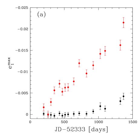
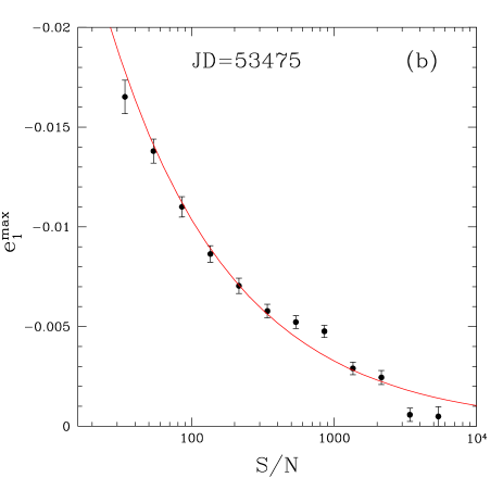
Figure 10.— Panel a: CTE induced polarization at the center of the exposure (maximum distance from the read-out electronics), as a function of time. The black points correspond to stars with a signal-to-noise ratio of $\sim 4000$, whereas the red points show the trend for $S/N\sim 40$. The results are consistent with a linear increase with time. Panel b: maximum CTE induced polarization as a function of S/N ratio at the mean Modified Julian Date of our cluster observations. The red curve is the best fit model $\propto\sqrt{S/N}$. Note that this scaling is different from Rhodes et al. (2007).

We use observations of the star cluster NGC104, which has been observed at regular epochs for a program to study the stability of ACS photometry. We select only the data with exposure times of 30s, which yields a uniform data set of 17 exposures, of which we omit one. These single exposures are drizzled and we measure the shape parameters from these images. The PSF anisotropy model for each exposure is determined using stars with $F814W<18$, as the effects of CTE are expected to be small for such bright objects. The fainter stars are corrected for PSF anisotropy and we measure $e_{1}$ as a function of $y$ coordinate.

We assume that the pattern is the same for each ACS chip and combine the data. We note that this assumption is actually supported by our measurements. For each exposure we fit a linear trend with distance from the read-out electronics

$$e_{1}^{\rm CTE}=e_{1}^{\rm max}(y/2048),$$

where $e_{1}^{\rm max}$ is the the maximum induced polarization. Figure 10(a) shows the resulting value for $e_{1}^{\rm max}$ as a function of time for stars with high (black points) and low (red points) signal-to-noise ratios. These measurements are consistent with a linear increase with time of the CTE induced distortion.

As expected the CTE effects are also more pronounced for fainter objects. To investigate this trend further, we compute $e_{1}^{\rm max}$ as a function of signal-to-noise ratio, adopting the average Modified Julian Date of our cluster observations. The results are shown in Figure 10(b). We fit the following model to our measurements

$$e_{1}^{\rm CTE}=e_{1}^{\rm max}\frac{1}{\sqrt{S/N}}\left(\frac{y}{2048}\right)(MJD-52,333).$$ (A1)

The red line in Figure 10(b) corresponds to the best model, for which we find $e_{1}^{\rm max}=(-9.07\pm 0.16)\times 10^{-5}$. Note that we have assumed that the CTE effect is proportional to $\sqrt{S/N}$, which is different from Rhodes et al. (2007) who argue for a scaling $\propto(S/N)^{-1}$. The latter scaling, however, is inconsistent with our findings. We have confirmed our results with other stellar fields. We note that Rhodes et al. (2007) use a different shape measurement method, which may explain some of the differences.

We now have an accurate model for the effects of CTE for stellar images, but it is not clear whether it is adequate for galaxies, which are more extended. Our cluster data cannot be used for this test, because the lensing signal induced by the clusters leads to a comparable change in $e_{1}$ with $y$ position. Instead we retrieved 100 pointings taken as part of the COSMOS survey (PID:10092) and analysed these data in a similar fashion as our own.

Figure 11 shows the measurement of $e_{1}^{\rm max}$ as a function of galaxy size $r_{g}$ for a signal-to-noise ratio of 20 and a mean modified Julian date of 53195. The points have been corrected for the small increase in mean S/N ratio as $r_{g}$ increases. The left-most point is the result derived from NGC104. We detect a clear size dependence of the CTE signal. We assume the dependence is a power-law, and we find a best fit slope of $-1.85\pm 0.3$; the best fit model is indicated by the solid line in Figure 11. We therefore revise our PSF-based model to account for the size dependence of the CTE effect:

$$e_{1}^{\rm CTE}=e_{1}^{\rm max}\frac{1}{\sqrt{S/N}}\left(\frac{y}{2048}\right)\left(\frac{r_{g}}{0.05^{\prime\prime}}\right)^{-1.85}(MJD-52,333),$$ (A2)

where the best fit value for $e_{1}^{\rm max}=(-8.3\pm 0.14)\times 10^{-5}$. This model is used to correct the observed $e_{1}$ for stars and galaxies in our data.

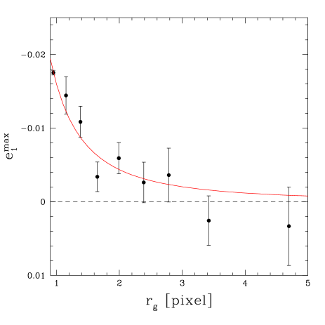
Figure 11.— Maximum CTE induced polarization as a function of galaxy size $r_{g}$ (for a S/N=20 and MJD=53195) based on the analysis of 100 pointings of the COSMOS survey. The left most point corresponds to the results from our analysis of star fields. We detect a clear dependence on size. The best fit power-law model is indicated by the solid line and has a slope $\sim-2$.

References

- Bardeau et al. (2007) Bardeau, S., Soucail, G., Kneib, J., Czoske, O., Ebeling, H., Hudelot, P., Smail, I., & Smith, G. P. 2007, A&A, 470, 449
- Bertin & Arnouts (1996) Bertin, E. & Arnouts, S. 1996, A&AS, 117, 393
- Bildfell et al. (2008) Bildfell, C., Hoekstra, H., Babul, A., & Mahdavi, A. 2008, MNRAS, 389, 1637
- Borgani et al. (2001) Borgani, S., Rosati, P., Tozzi, P., Stanford, S. A., Eisenhardt, P. R., Lidman, C., Holden, B., Della Ceca, R., Norman, C., & Squires, G. 2001, ApJ, 561, 13
- Bower et al. (2008) Bower, R. G., McCarthy, I. G., & Benson, A. J. 2008, MNRAS, 390, 1399
- Bruch et al. (2010) Bruch, S., Donahue, M., Voit, G., Sun, M., & Conselice, C. 2010, ApJ, submitted
- Bryan & Norman (1998) Bryan, G. L. & Norman, M. L. 1998, ApJ, 495, 80
- Carrasco et al. (2007) Carrasco, E. R., Cypriano, E. S., Neto, G. B. L., Cuevas, H., Sodré, Jr., L., de Oliveira, C. M., & Ramirez, A. 2007, ApJ, 664, 777
- Duffy et al. (2008) Duffy, A. R., Schaye, J., Kay, S. T., & Dalla Vecchia, C. 2008, MNRAS, 390, L64
- Evrard et al. (2002) Evrard, A. E., MacFarland, T. J., Couchman, H. M. P., Colberg, J. M., Yoshida, N., White, S. D. M., Jenkins, A., Frenk, C. S., Pearce, F. R., Peacock, J. A., & Thomas, P. A. 2002, ApJ, 573, 7
- Evrard et al. (1996) Evrard, A. E., Metzler, C. A., & Navarro, J. F. 1996, ApJ, 469, 494
- Fernández-Soto et al. (1999) Fernández-Soto, A., Lanzetta, K. M., & Yahil, A. 1999, ApJ, 513, 34
- Gladders et al. (2007) Gladders, M. D., Yee, H. K. C., Majumdar, S., Barrientos, L. F., Hoekstra, H., Hall, P. B., & Infante, L. 2007, ApJ, 655, 128
- Henry (2000) Henry, J. P. 2000, ApJ, 534, 565
- Henry (2004) —. 2004, ApJ, 609, 603
- Henry et al. (2009) Henry, J. P., Evrard, A. E., Hoekstra, H., Babul, A., & Mahdavi, A. 2009, ApJ, 691, 1307
- Hoekstra (2001) Hoekstra, H. 2001, A&A, 370, 743
- Hoekstra (2003) —. 2003, MNRAS, 339, 1155
- Hoekstra (2007) —. 2007, MNRAS, 379, 317
- Hoekstra et al. (2000) Hoekstra, H., Franx, M., & Kuijken, K. 2000, ApJ, 532, 88
- Hoekstra et al. (1998) Hoekstra, H., Franx, M., Kuijken, K., & Squires, G. 1998, ApJ, 504, 636
- Hoekstra et al. (2002) Hoekstra, H., Franx, M., Kuijken, K., & van Dokkum, P. G. 2002, MNRAS, 333, 911
- Hoekstra & Jain (2008) Hoekstra, H. & Jain, B. 2008, Annual Review of Nuclear and Particle Science, 58, 99
- Horner (2001) Horner, D. J. 2001, PhD thesis, University of Maryland College Park
- Ilbert et al. (2006) Ilbert, O., Arnouts, S., McCracken, H. J., Bolzonella, M., Bertin, E., Le Fèvre, O., Mellier, Y., Zamorani, G., Pellò, R., Iovino, A., Tresse, L., Le Brun, V., Bottini, D., Garilli, B., Maccagni, D., Picat, J. P., Scaramella, R., Scodeggio, M., Vettolani, G., Zanichelli, A., Adami, C., Bardelli, S., Cappi, A., Charlot, S., Ciliegi, P., Contini, T., Cucciati, O., Foucaud, S., Franzetti, P., Gavignaud, I., Guzzo, L., Marano, B., Marinoni, C., Mazure, A., Meneux, B., Merighi, R., Paltani, S., Pollo, A., Pozzetti, L., Radovich, M., Zucca, E., Bondi, M., Bongiorno, A., Busarello, G., de La Torre, S., Gregorini, L., Lamareille, F., Mathez, G., Merluzzi, P., Ripepi, V., Rizzo, D., & Vergani, D. 2006, A&A, 457, 841
- Johnston et al. (2007) Johnston, D. E., Sheldon, E. S., Wechsler, R. H., Rozo, E., Koester, B. P., Frieman, J. A., McKay, T. A., Evrard, A. E., Becker, M. R., & Annis, J. 2007, ArXiv e-prints
- Kaiser (1986) Kaiser, N. 1986, MNRAS, 222, 323
- Kaiser et al. (1995) Kaiser, N., Squires, G., & Broadhurst, T. 1995, ApJ, 449, 460
- Koekemoer et al. (2002) Koekemoer, A. M., Fruchter, A. S., Hook, R. N., & Hack, W. 2002, in The 2002 HST Calibration Workshop : Hubble after the Installation of the ACS and the NICMOS Cooling System, ed. S. Arribas, A. Koekemoer, & B. Whitmore, 337–+
- Koester et al. (2007) Koester, B. P., McKay, T. A., Annis, J., Wechsler, R. H., Evrard, A., Bleem, L., Becker, M., Johnston, D., Sheldon, E., Nichol, R., Miller, C., Scranton, R., Bahcall, N., Barentine, J., Brewington, H., Brinkmann, J., Harvanek, M., Kleinman, S., Krzesinski, J., Long, D., Nitta, A., Schneider, D. P., Sneddin, S., Voges, W., & York, D. 2007, ApJ, 660, 239
- Komatsu et al. (2009) Komatsu, E., Dunkley, J., Nolta, M. R., Bennett, C. L., Gold, B., Hinshaw, G., Jarosik, N., Larson, D., Limon, M., Page, L., Spergel, D. N., Halpern, M., Hill, R. S., Kogut, A., Meyer, S. S., Tucker, G. S., Weiland, J. L., Wollack, E., & Wright, E. L. 2009, ApJS, 180, 330
- Leauthaud et al. (2010) Leauthaud, A., Finoguenov, A., Kneib, J., Taylor, J. E., Massey, R., Rhodes, J., Ilbert, O., Bundy, K., Tinker, J., George, M. R., Capak, P., Koekemoer, A. M., Johnston, D. E., Zhang, Y., Cappelluti, N., Ellis, R. S., Elvis, M., Giodini, S., Heymans, C., Le Fèvre, O., Lilly, S., McCracken, H. J., Mellier, Y., Réfrégier, A., Salvato, M., Scoville, N., Smoot, G., Tanaka, M., Van Waerbeke, L., & Wolk, M. 2010, ApJ, 709, 97
- Lumb et al. (2004) Lumb, D. H., Bartlett, J. G., Romer, A. K., Blanchard, A., Burke, D. J., Collins, C. A., Nichol, R. C., Giard, M., Marty, P. B., Nevalainen, J., Sadat, R., & Vauclair, S. C. 2004, A&A, 420, 853
- Luppino & Kaiser (1997) Luppino, G. A. & Kaiser, N. 1997, ApJ, 475, 20
- Mahdavi et al. (2008) Mahdavi, A., Hoekstra, H., Babul, A., & Henry, J. P. 2008, MNRAS, 384, 1567
- Mandelbaum et al. (2008a) Mandelbaum, R., Seljak, U., & Hirata, C. M. 2008a, JCAP, 8, 6
- Mandelbaum et al. (2008b) Mandelbaum, R., Seljak, U., Hirata, C. M., Bardelli, S., Bolzonella, M., Bongiorno, A., Carollo, M., Contini, T., Cunha, C. E., Garilli, B., Iovino, A., Kampczyk, P., Kneib, J., Knobel, C., Koo, D. C., Lamareille, F., Le Fèvre, O., Le Borgne, J., Lilly, S. J., Maier, C., Mainieri, V., Mignoli, M., Newman, J. A., Oesch, P. A., Perez-Montero, E., Ricciardelli, E., Scodeggio, M., Silverman, J., & Tasca, L. 2008b, MNRAS, 386, 781
- Mantz et al. (2010a) Mantz, A., Allen, S. W., Ebeling, H., Rapetti, D., & Drlica-Wagner, A. 2010a, MNRAS, 1030
- Mantz et al. (2010b) Mantz, A., Allen, S. W., Rapetti, D., & Ebeling, H. 2010b, MNRAS, 1029
- Massey et al. (2007) Massey, R., Rhodes, J., Leauthaud, A., Capak, P., Ellis, R., Koekemoer, A., Réfrégier, A., Scoville, N., Taylor, J. E., Albert, J., Bergé, J., Heymans, C., Johnston, D., Kneib, J., Mellier, Y., Mobasher, B., Semboloni, E., Shopbell, P., Tasca, L., & Van Waerbeke, L. 2007, ApJS, 172, 239
- Massey et al. (2010) Massey, R., Stoughton, C., Leauthaud, A., Rhodes, J., Koekemoer, A., Ellis, R., & Shaghoulian, E. 2010, MNRAS, 401, 371
- Mullis et al. (2003) Mullis, C. R., McNamara, B. R., Quintana, H., Vikhlinin, A., Henry, J. P., Gioia, I. M., Hornstrup, A., Forman, W., & Jones, C. 2003, ApJ, 594, 154
- Nagai et al. (2007) Nagai, D., Vikhlinin, A., & Kravtsov, A. V. 2007, ApJ, 655, 98
- Navarro et al. (1997) Navarro, J. F., Frenk, C. S., & White, S. D. M. 1997, ApJ, 490, 493
- Rasia et al. (2006) Rasia, E., Ettori, S., Moscardini, L., Mazzotta, P., Borgani, S., Dolag, K., Tormen, G., Cheng, L. M., & Diaferio, A. 2006, MNRAS, 369, 2013