Leverage Bubble

Abstract

Leverage is strongly related to liquidity in a market and lack of liquidity is considered a cause and/or consequence of the recent financial crisis. A repurchase agreement is a financial instrument where a security is sold simultaneously with an agreement to buy it back at a later date. Repurchase agreements (repos) market size is a very important element in calculating the overall leverage in a financial market. Therefore, studying the behavior of repos market size can help to understand a process that can contribute to the birth of a financial crisis. We hypothesize that herding behavior among large investors led to massive over-leveraging through the use of repos, resulting in a bubble (built up over the previous years) and subsequent crash in this market in early 2008. We use the Johansen-Ledoit-Sornette (JLS) model of rational expectation bubbles and behavioral finance to study the dynamics of the repo market that led to the crash. The JLS model qualifies a bubble by the presence of characteristic patterns in the price dynamics, called log-periodic power law (LPPL) behavior. We show that there was significant LPPL behavior in the market before that crash and that the predicted range of times predicted by the model for the end of the bubble is consistent with the observations.

url]http://www.er.ethz.ch/

1 Introduction

Financial bubbles play a huge role in the global economy, affecting hundreds of millions of people yet, until recently, the existence of such bubbles, much less their effects, have been ignored at the policy level. Finally, only after this most recent historical global financial crisis (which is still ongoing), officials at the highest level of government and academic finance have acknowledged the existence and importance of identifying and understanding bubbles. No less than the President of the Federal Reserve Bank of New York, William C. Dudley, stated just a few months ago [1]:

$\ldots$what I am proposing is that we try—try to identify bubbles in real time, try to develop tools to address those bubbles, try to use those tools when appropriate to limit the size of those bubbles and, therefore, try to limit the damage when those bubbles burst.

Such a statement from the New York Fed—representing, essentially, the monetary policy of the United States governmental banking system—would have been, and, in some circles, still is, unheard of. This, in short, is a bombshell and a wake-up call to academics and practitioners. Dudley proposes to “try to develop tools to address…bubbles”. Before discussing tools that could address bubbles, we must know what a bubble is.

A financial bubble is a curious beast: its meaning is accepted as beyond obvious by average people yet its very existence is loudly debated in angry terms among experts. Arguably, almost any given adult met on the street in, say Asia, Europe or North America (and, or course, elsewhere), would know exactly what one is and could cite examples in recent and distant history. The dot.com bubble ending in 2000 and the housing bubble recently ended would most likely be the most common examples given. More well-read—but still non-expert—people could cite the Dutch tulip mania in the 1600s and the South Sea Company of the 1700s. After that, the examples are less well-known but not because of their scarcity but just because most people are not interested in financial history and debates. This is changing.

While the general population accepts bubbles, academics and policy-makers have a decades-old tradition of arguing about whether bubbles even exist. This single fact could very well be the most striking and unbelievable statement ever transmitted from the Ivory Tower. In spite of the lack of academic consensus on a definition, we can give a qualitative ideas of bubbles and apply our quantitative approach in the next sections. Following [2], the term “bubble” refers to a situation in which excessive public expectations of future price increases cause prices to be temporarily elevated. For instance, during a housing price bubble, homebuyers think that a home that they would normally consider too expensive for them is now an acceptable purchase because they will be compensated by significant further price increases. They will not need to save as much as they otherwise might, because they expect the increased value of their home to do the saving for them. First-time homebuyers may also worry during a housing bubble that if they do not buy now, they will not be able to afford a home later. Furthermore, the expectation of large price increases may have a strong impact on demand if people think that home prices are very unlikely to fall, and certainly not likely to fall for long, so that there is little perceived risk associated with an investment in a home.

In this paper, instead of a housing bubble, we argue that there was a leverage bubble that peaked and crashed in early 2008 after building up for the years beforehand. As we explain below, the leverage bubble formed and grew for the same reasons as described in the housing bubble example above: investors were afraid that if they did not extend their leverage (buy a house) then they would lose money later. Further, we argue that the size of the market in repurchase agreements (or repos, for short) is an observable proxy of leverage in the financial system. We will elaborate on repos below, but, briefly, a repo is simply a cash transaction for an asset combined with a forward contract to buy the asset back at a later time (hence ‘re-purchase’). By measuring the size of the repos market and applying an appropriate bubble model, we can see that the leverage crash in early 2008 was potentially a forecastable event.

The paper is constructed as follows: in Section 2, we discuss the relationship between repos market size and the overall leverage of the market. In Section 3, we briefly introduce the Johansen-Ledoit-Sornette model [3, 4] of bubbles and apply it to total repos market size to make an ex-post forecast of the crash in early 2008. We conclude in Section 4.

2 Repos market size represents the leverage of the market

A repurchase agreement (repo) is the sale of securities together with an agreement for the seller to buy back the securities at a later date [5]. In other words, it is a contract obliging the seller of an asset to buy back the asset at a specified price on a given date. Therefore, a repo is equivalent to a cash transaction combined with a forward contract. The cash transaction results in transfer of money to the borrower in exchange for legal transfer of the security to the lender, while the forward contract ensures repayment of the loan to the lender and return of the collateral of the borrower.

To understand the possible role of repos in the generation of a bubble, we first discuss the relationship between leverage and balance sheet size. We start with a very simple case, taken from Section 2 of [6]. Assume that an investment bank has 100 USD in securities while its shareholder equity is 20 USD and its debt is 80 USD. Then the balance sheet of this bank looks like:

Assets	Liabilities
Securities, 100	Equity, 20
	Debt, 80

Now the leverage of the bank is:

$$\frac{assets}{equity}=\frac{100}{20}=5.$$ (1)

Suppose that the debts of this bank are all long term debts and, therefore, we can assume that the debt remains the same in the balance sheet over the short period of time considered in the argument. Now assume that the prices of the securities increase by 10%, so that the new balance sheet is:

Assets	Liabilities
Securities, 110	Equity, 30
	Debt, 80

The leverage, then, becomes:

$$\frac{assets}{equity}=\frac{110}{30}=3.67<5.$$ (2)

This shows that the leverage decreases as the assets’ prices increase.

However, to an investor during the bull market, reduction of the leverage means losing money. Consider another example to demonstrate this. Suppose that two people $A$ and $B$ both have a house worth 1000 USD. Assume that they somehow know that the price of gold, for instance, will definitely increase in the near future. Each of them can use her house as collateral and get a maximum 2000 USD load from a bank (based on the recent convention of poor underwriting requirements). Investor $A$, being somewhat unsure of her future ability to repay her debts, applied for and received ‘only’ 1500 USD, which corresponds to a leverage of 1.5. Investor $B$, though, with no such qualms, asked for and received the maximum value of 2000 USD, for a leverage of 2. Both investors used all of the borrowed money to buy gold. After one month, the gold price, as expected, increased by 20%. Both $A$ and $B$ sold all of the leveraged gold and repurchased their respective houses for 1000 USD (ignore interest rate for simplicity). Investor $A$ has made a profit of 800 USD but investor $B$, the bold risk-taker, has made almost double the profit of 1400 USD by simply increasing her leverage by one-third. In a sense, investor $A$’s weak-kneed approach lost 600 USD due to failure to maximally leverage her position.

With this lesson in mind, let us now return to the investment bank. During the bull market, banks believe that the markets will continue to increase and that all of their competitors will be maximally leveraged to take advantage of the expected rise. If a bank decreases its leverage, it means it will lose money in the future so, guided by the practice of maximizing short-term profits by any means necessary, banks increase their leverage in order to get more return in the future. How large they will increase their leverage depends on their expectation of the future market. If the market performs very well now, they expect that the future will be very good, also. This means that they will change their leverage based on the return now. Regardless of whether this is a good thing or not, for our study, we can use this because it implies that the total asset growth should be proportional to the leverage growth. This is demonstrated in Fig. 8 of [6]. In that paper, the authors used quarterly data from more than 10 years for six major U.S. investment banks: Lehman Brothers, Merrill Lynch, Morgan Stanley, Bear Stearns, Goldman Sachs and Citigroup Markets. The total asset growth of the banks is found strongly proportional to the leverage growth. So we know that when the expectation of the market is high, the investment banks tend to increase their leverage. The next question, then, is: how can a bank change its leverage?

Repos play a key role here. A typical balance sheet of an investment bank has not only the long term debt but also repos. Therefore, a typical balance sheet is as follows:

Assets	Liabilities
Trading assets	Repos
Reverse repos	Long term debt
Other assets	Equity

Recall that a repo is the sale of securities together with an agreement for the seller to buy back the securities at a later date. Long term debt is normally a small fraction of the balance sheet and can be assumed to be constant over the time scale of interest here (a few years at most). In this case, when banks want to increase or decrease their leverage, they will write repos.

One may argue that the haircut of the repo is also a very important role for the leverage of the banks. We completely agree with this and the repurchase haircut should be counted here. However, the historical data shows that the haircut remains approximately within a range between 10% and 20% during ‘normal’ (i.e., non-crisis) times. During a financial crisis, the haircut will rise sharply to a very high level. When there is a shortage of liquidity, for instance, during the recent financial crisis, investors are afraid to trade. Increased haircuts and decreased repos size usually occur simultaneously. In this paper, we want to investigate the question of whether or not the dynamics of repos activity shows any precursory information before a large crash. Of course, this means we only use data before a crash to try to estimate the time of its onset. Since the haircut is almost constant for a long time before a crash, all of the leverage information lies in the repo size of the market.

To summarize this section, we claim that:

1. investors want to increase their leverage when their expectations of future gains of the market increase;

2. they will use repos to increase their leverage;

3. therefore, the total repo market size is a proxy to measure the overall expectation of all investors.

3 Predicting financial crashes with the Johansen-Ledoit-Sornette model

In the last section, we said that the repos market size represents the average leverage of the market and the leverage represents the investors’ expectation of future market returns. We now discuss how the dynamics of leverage among traders could lead to a bubble and how this bubble can be identified as it grows.

We have argued before that bubbles are the result of imitation and herding behavior among investors [7, 3, 4, 8]. In the current case, investors increase their leverage when they see others doing so because, as discussed above, they think that they will lose money if they are the only ones not taking this strategy. Of course, this is a self-reinforcing (positive feedback) process: the numbers of leveraged investors and their levels of leverage will increase in a game of financial copycat. At some point, though, some investors are bound to notice that the numbers are too large and they will start to deleverage. Others nervously waiting for this signal will unload as well and the bottom will drop out. When this occurs, the repo market size goes down dramatically and the haircut of the repo increases very sharply, both leading to rapid loss of liquidity in the repo market.

This qualitative process is quantified in the Johansen-Ledoit-Sornette (JLS) model to describe the herding dynamics during a bubble [3, 4]. This model combines the economic theory of rational expectation bubbles, behavioral finance on imitation and herding of investors and traders and the mathematical and statistical physics of bifurcations and phase transitions. Many successful predictions of financial market crashes based on this model have been made, such as the 2006–2008 oil bubble [9], the Chinese index bubble in 2009 [10], real estate market in Las Vegas [11], South African stock market bubble [12]. Also, new methods using this model to predict stock market rebounds rather than the crashes are being developed [13].

In the JLS model, (the logarithm of) price is used as a proxy for herding behavior among traders (see [14] for justifications on the use of log-price versus price). Since we argue that the repo market size is also a proxy for herding via the leverage level, we substitute it for the log-price in the JLS model. For the total repos market size $R(t)$ at time $t$, we use the following JLS model specification (corresponding to replace log-price by repos volume in the JLS equation):

$$R(t)=A+B|t_{c}-t|^{m}+C|t_{c}-t|^{m}\cos(\ln\omega|t_{c}-t|+\phi)~{},$$ (3)

where $t_{c}$ is the crash time and $m,\omega,\phi,A,B$ and $C$ are parameters. To determine the values of these parameters, we want to minimize the sum of squares:

$$(t_{c},m,\omega,\phi,A,B,C)=$$ (4)

$$\arg\min\sum_{t}(R(t)-A+B|t_{c}-t|^{m}+C|t_{c}-t|^{m}\cos(\ln\omega|t_{c}-t|+\phi))^{2}~{}.$$

We hypothesize that the run-up to the sudden large drop in the repos market in early 2008 was characterized by LPPL dynamics, supporting our claim of the entanglement of expectations, leverage and herding behavior.

To test this hypothesis, we use the weekly data of US primary dealers’ total repos size from 6 July 1994 to 23 June 2010. The data have very strong seasonal effects due to the fact that banks try to remove their repos to improve their balance sheet at the end of each quarter. To remove the seasonal effect, we used a 13 week (1 quarter) moving average.

We fit this smoothed time series with the JLS equation (3) in time windows defined by $(t_{1},t_{2})$. We chose a fixed $t_{2}=$ 13 February 2008, approximately one month before the observed peak of the repos volume. We then repeated the analysis with an ensemble of 7 values of $t_{2}$, each separated by 7 days for the 3 weeks before and after 13 February 2008. Note that the 7 values of $t_{2}$ bracket a time span of 6 weeks, with the end of that period (5 March 2008) being just before the large drop in the repos market. Also note that an observer in the past on this date would not have noticed any unusual drop in the time series. That is, the impending crash was not obvious based on any recent trend in the data (though perhaps some market intelligence could have provided an indication). For each value of $t_{2}$, we use an ensemble of different $t_{1}$’s. Each ensemble brackets a range between 6 and 18 months before the respective $t_{2}$ and values of $t_{1}$ are separated by 7 days.

The fit for a particular $(t_{1},t_{2})$ interval is generated in two steps. First, the linear parameters $A,B$ and $C$ are slaved to the non-linear parameters by solving them analytically as a function of the nonlinear parameters. We refer to [3] (page 238 and following ones), which gives the detailed equations and procedure. Then, the search space is obtained as a 4 dimensional parameter space representing $m,\omega,\phi$ and $t_{c}$. A heuristic search implementing the Taboo algorithm [15] is used to find 10 initial estimates of the parameters which are then passed to a Levenberg-Marquardt algorithm [16, 17] to minimize the residuals (the sum of the squares of the differences) between the model and the data. The bounds of the search space are:

$$m \in [0.001,1.999]$$ (5)

$$\omega \in [0.01,40]$$ (6)

$$\phi \in [0.001,2\pi-0.001]$$ (7)

$$t_{c} \in [t_{2},t_{2}+0.375(t_{2}-t_{1})]$$ (8)

Fig.1 shows the fitting results with a fixed end of the time series $t_{2}$ = 3 February 2008 and the ensemble of $t_{1}$s as described above. The use of many fits provides an ensemble of $t_{c}$’s, from which we can calculate quantiles of the most likely date of a crash. The 20%-80% quantile region is shown on the figure as the inner vertical band with diagonal cross-hatching. The 5%-95% quantiles are shown as the outer vertical band with horizontal hatching. The dark vertical line to the left of the quantile windows represent the last observation used in the analysis, that is, $t_{2}$. The shaded envelopes to the right of $t_{2}$ represent 20%-80% and 5%-95% quantiles of the extrapolations of the fits. From the plot, we see that both the $t_{c}$ quantiles and the extrapolation quantiles are consistent with the observed trajectory of the moving average of the repos market size.

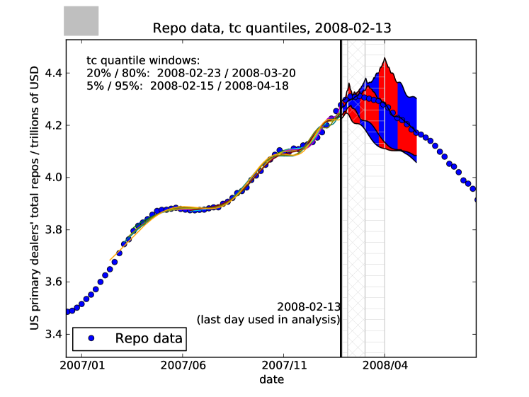
Figure 1: Results of the calibration of the JLS model calibrated to the time evolution of the total repos market size. The end time of the time series is fixed to $t_{2}=$2008-02-03, shown as the dark vertical line to the left of the quantile windows. For different starting time, the probability density of the crash time $t_{c}$ is shown in quantiles. The curves on the right of the dark vertical line are the extrapolated quantile repos volume, which are found consistent with the realized trajectory of the moving average of the repos market size.

Our use of 7 values of $t_{2}$’s in the 6 week window described above is to address the issue of the stability of the predicted crash time in relation to $t_{2}$. We fit the ensemble of $(t_{1},t_{2})$ intervals as described above and plot the pdf’s of the predicted crash time $t_{c}$ for each $t_{2}$. The result is shown in Fig. 2. From the plot, one can observe two regimes. The first four pdf’s corresponding to the earliest $t_{2}$’s peak practically at the same value, showing a very good stability. The last two pdf’s show a tendency to shift to the future, as some of the used data starts to be sensitive to the plateauing of the repos volume. Overall, the observed stability of the predicted distributions of $t_{c}$’s means the calibration of the JLS model is quite insensitive with when the prediction is made. This is proposed as an important validation step for the relevance of the JLS model. This suggests that the JLS model can be used for advance diagnostic of impending crashes. The present results add to those accumulating within the “financial bubble experiment”, which has the goal of constructing advanced forecasts of bubbles and crashes. In the financial bubble experiment, the results are revealed only after the predicted event has passed but the original date when we produced the forecasts has been publicly, digitally authenticated [18, 19].

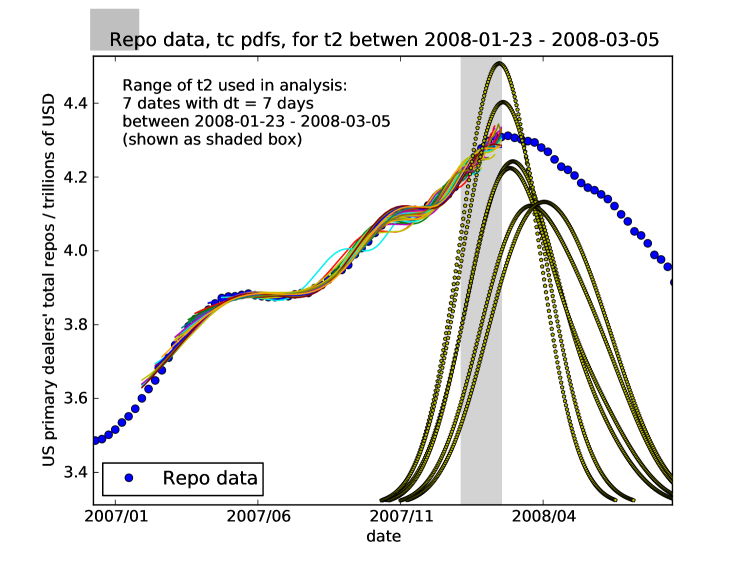
Figure 2: We vary the end of the window $t_{2}$ within the grey area and show the probability density of the crash time $t_{c}$ for each of these $t_{2}$, as the bell-shaped curves with open circle symbols.

4 Conclusion

In this paper, we discussed how leverage can influence the liquidity of the market and used the observation that a dramatic decrease of leverage coincides with the recent financial crisis. The market size of repos is a very good proxy for the overall leverage of the market. We used the JLS model of log-periodic power law dynamics on an ensemble of intervals from a time series of the total repos market size and found that the range of crash times $t_{c}$ as forecast by the fits is consistent with the observed peak and subsequent crash.

References

- Dudley [2010] W. C. Dudley, The friday podcast: New york fed chief, bubble fighter, NPR Planet Money (2010).
- Case and Shiller [2003] K. E. Case, R. J. Shiller, Is there a bubble in the housing market, Brookings Papers Econ. Activity (2) (2003) 299–362.
- Johansen et al. [1999] A. Johansen, D. Sornette, O. Ledoit, Predicting financial crashes using discrete scale invariance, Journal of Risk 1 (1999) 5–32.
- Johansen et al. [2000] A. Johansen, O. Ledoit, D. Sornette, Crashes as critical points, International Journal of Theoretical and Applied Finance 3 (2000) 219–255.
- wikipedia repo [page] wikipedia repo, : http://en.wikipedia.org/wiki/Repurchase_agreement (webpage).
- Adrian and Shin [2010] T. Adrian, H.-S. Shin, Liquidity and leverage, Journal of Financial Intermediation 19 (2010) 418–437.
- Sornette et al. [1996] D. Sornette, A. Johansen, J. P. Bouchaud, Stock market crashes, precursors and replicas, J. Phys. I France 6 (1996) 167–175.
- Sornette [2003] D. Sornette, Why stock markets crash (critical events in complex financial systems), Why Stock Markets Crash (Critical Events in Complex Financial Systems), Princeton University Press (2003).
- Sornette et al. [2009] D. Sornette, R. Woodard, W.-X. Zhou, The 2006-2008 oil bubble: evidence of speculation and prediction, Physica A 388 (2009) 1571–1576.
- Jiang et al. [2010] Z.-Q. Jiang, W.-X. Zhou, D. Sornette, R. Woodard, K. Bastiaensen, P. Cauwels, Bubble diagnosis and prediction of the 2005-2007 and 2008-2009 chinese stock market bubbles, Journal of Economic Behavior and Organization 74 (2010) 149–162.
- Zhou and Sornette [2008] W.-X. Zhou, D. Sornette, Analysis of the real estate market in las vegas: Bubble, seasonal patterns, and prediction of the csw indexes, Physica A 387 (2008) 243–260.
- Zhou and Sornette [2006] W.-X. Zhou, D. Sornette, A case study of speculative financial bubbles in the south african stock market 2003-2006, Physica A 361 (2006) 297–308.
- Yan et al. [2010] W. Yan, R. Woodard, D. Sornette, Diagnosis and prediction of market rebounds in financial markets, international journal of forecasting, New Journal of Physics submitted (2010). Http://arxiv.org/abs/1001.0265.
- Johansen and Sornette [1999] A. Johansen, D. Sornette, Critical crashes, Risk 12 (1999) 91–94.
- Cvijovic and Klinowski [1995] D. Cvijovic, J. Klinowski, Taboo search: an approach to the multiple minima problem, Science 267 (1995) 664–666.
- Levenberg [1944] K. Levenberg, A method for the solution of certain non-linear problems in least squares, Quarterly Journal of Applied Mathematics II 2 (1944) 164–168.
- Marquardt [1963] D. W. Marquardt, An algorithm for least-squares estimation of nonlinear parameters, Journal of the Society for Industrial and Applied Mathematics 11 (1963) 431–441.
- Sornette et al. [2010a] D. Sornette, R. Woodard, M. Fedorovsky, S. Reimann, H. Woodard, W.-X. Zhou, The financial bubble experiment: advanced diagnostics and forecasts of bubble terminations (the financial crisis observatory), http://arxiv.org/abs/0911.0454 (2010a).
- Sornette et al. [2010b] D. Sornette, R. Woodard, M. Fedorovsky, S. Reimann, H. Woodard, W.-X. Zhou, The financial bubble experiment: Advanced diagnostics and forecasts of bubble terminations volume ii–master document, http://arxiv.org/abs/1005.5675 (2010b).