Axial and pseudoscalar form-factors of the $\Delta^{+}(1232)$

Abstract:

We present first results on the axial and pseudoscalar $\Delta$ form factors. The analysis is carried out in the quenched approximation where statistical errors are small and the lattice set-up can be investigated relatively quickly. We also present an analysis with a hybrid action using staggered sea quarks and domain-wall valence fermions.

1 Introduction

A major focus of interest in hadronic physics is the quest to understand from first principles the structure of mesons and baryons. In particular form factors yield information about the size and shape of the hadrons.

Much theoretical and experimental work has gone into understanding the structure of nucleons and the $N\rightarrow\Delta$ transition. Lattice QCD calculations of the nucleon and $N\rightarrow\Delta$ form factors (FFs) have been carried out within the same lattice setup as the one used in this work [1, 2, 3]. Experimental information on the FFs of $\Delta(1232)$ is scarce due to its short lifetime ($\sim 10^{-23}$ s) [5, 6]. However, in a finite-volume simulation with heavy pions, the $\Delta$ is stable and accessible to lattice techniques. A pioneering lattice study [4] investigated the electromagnetic form-factors of the $\Delta$ in the quenched approximation. Recently, a state-of-the-art lattice calculation of the electromagnetic FFs of the $\Delta$ and the associated transverse charge densities in the infinite momentum frame has been carried out [7]. In this report we extend the effort to the axial and pseudoscalar form factors of the $\Delta(1232)$ and present preliminary results. To our knowledge this is the first time that these FFs have been computed.

Despite the difficulty of experimental confirmation of these results, they can yield an evaluation of the axial charge and the effective $\pi\Delta\Delta$ couplings, parameters which can be fed into chiral expansions to aid the chiral extrapolations of, for example, the nucleon axial charge. The axial Ward-Takahashi identity relates the axial FFs to the pseudoscalar FFs. As in the nucleon case, one can derive the generalized Goldberger-Treiman relations. In this work we derive these and check their validity.

2 Lattice calculation

This project closely follows the methods used for extracting $\Delta^{+}$ electromagnetic form factors as described comprehensively in Ref. [7]. We begin with the expression of the isovector axial vertex:

$$\langle\Delta(p_{f},s_{f})|A^{\mu}|\Delta(p_{i},s_{i})\rangle=\overline{u}_{\alpha}(p_{f},s_{f})\left[{\mathcal{O}}^{\mu{\rm A}}\right]^{\alpha\beta}u_{\beta}(p_{i},s_{i}),$$ (1)

with

$$A^{\mu}(x)=\overline{\psi}(x)\gamma^{\mu}\gamma_{5}\frac{\tau^{3}}{2}\psi(x).$$

The right-hand side is an expression containing the most general decomposition of the axial vertex in terms of four form-factors, which we label $g_{1}$, $g_{3}$, $h_{1}$ and $h_{3}$:

$${\mathcal{O}}^{\mu{\rm A}}=-g^{\alpha\beta}\left(g_{1}(q^{2})\gamma^{\mu}\gamma^{5}+g_{3}(q^{2})\frac{q^{\mu}}{2M_{\Delta}}\gamma^{5}\right)+\frac{\displaystyle q^{\alpha}q^{\beta}}{\displaystyle 4M_{\Delta}^{2}}\left(h_{1}(q^{2})\gamma^{\mu}\gamma^{5}+h_{3}(q^{2})\frac{q^{\mu}}{2M_{\Delta}}\gamma^{5}\right),$$ (2)

and $u_{\alpha}$ is the Rarita-Schwinger spinor and $q=p_{f}-p_{i}$.

Similarly we can write the pseudoscalar vertex in terms of two form-factors, $\tilde{g}$ and $\tilde{h}$:

$$\langle\Delta(p_{f},s_{f})|P|\Delta(p_{i},s_{i})\rangle=\overline{u}_{\alpha}(p_{f},s_{f})\left[{\mathcal{O}}^{{\rm PS}}\right]^{\alpha\beta}u_{\beta}(p_{i},s_{i})$$ (3)

with

$$P(x)=\overline{\psi}(x)\gamma_{5}\frac{\tau^{3}}{2}\psi(x)$$ (4)

and

$${\mathcal{O}}^{{\rm PS}}=-g^{\alpha\beta}\tilde{g}(q^{2})\gamma^{5}+\frac{\displaystyle q^{\alpha}q^{\beta}}{\displaystyle 4M_{\Delta}^{2}}\tilde{h}(q^{2})\gamma^{5}$$ (5)

We isolate the form-factors by constructing ratios of lattice two- and three-point functions. The standard lattice interpolating field with the $\Delta^{+}$ quantum numbers is given by

$${\bf\chi}^{\Delta^{+}}_{\sigma\alpha}(x)=\frac{1}{\sqrt{3}}\epsilon^{abc}\Bigl{[}2\left({\bf u}^{a\top}(x)C\gamma_{\sigma}{\bf d}^{b}(x)\right){\bf u}_{\alpha}^{c}(x)+\left({\bf u}^{a\top}(x)C\gamma_{\sigma}{\bf u}^{b}(x)\right){\bf d}_{\alpha}^{c}(x)\Bigr{]}\,.$$ (6)

The two-point and three-point functions of interest are:

$$G_{\sigma\mu\tau}^{X}(\Gamma^{\nu},\vec{q},t) = \sum_{\vec{x},\vec{x}_{f}}e^{+i\vec{x}\cdot\vec{q}}\Gamma^{\nu}_{\alpha^{\prime}\alpha}\langle\chi_{\sigma\alpha}(t_{f},\vec{x}_{f})X_{\mu}(t,\vec{x})\overline{\chi}_{\tau\alpha^{\prime}}(0,\vec{0})\rangle$$ (7)

$$G_{\sigma\tau}(\Gamma^{\nu},\vec{p},t) = \sum_{\vec{x}_{f}}e^{-i\vec{x}_{f}\cdot\vec{p}}\Gamma^{\nu}_{\alpha^{\prime}\alpha}\langle\chi_{\sigma\alpha}(t,\vec{x}_{f})\overline{\chi}_{\tau\alpha^{\prime}}(0,\vec{0})\rangle$$ (8)

where $X$ stands for the axial-vector and pseudo-scalar currents defined in Eqs. (2) and (4) respectively and

$$\Gamma^{4}=\frac{1}{4}({\bf 1}+\gamma^{4})\,,\qquad\qquad\Gamma^{k}=\frac{i}{4}({\bf 1}+\gamma^{4})\gamma_{5}\gamma_{k}\,,\qquad k=1,2,3\,.$$ (9)

We examine ratios of these to eliminate unknown $Z$-factors and leading time-dependence.:

$$R_{\sigma\mu\tau}^{X}(\Gamma,\vec{q},t)=\frac{G_{\sigma\mu\tau}^{X}(\Gamma,\vec{q},t)}{G_{kk}(\Gamma^{4},\vec{0},t_{f})}\ \sqrt{\frac{G_{kk}(\Gamma^{4},\vec{p}_{i},t_{f}-t)G_{kk}(\Gamma^{4},\vec{0},t)G_{kk}(\Gamma^{4},\vec{0},t_{f})}{G_{kk}(\Gamma^{4},\vec{0},t_{f}-t)G_{kk}(\Gamma^{4},\vec{p}_{i},t)G_{kk}(\Gamma^{4},\vec{p}_{i},t_{f})}}\,,$$

These ratios tend to a constant at large Euclidean time separations $t_{f}-t_{i}$ and $t$:

$$R_{\sigma(\mu)\tau}(\Gamma,\vec{q},t)^{X}\stackrel{{\scriptstyle{\tiny\begin{array}[]{c}t_{f}-t\rightarrow\infty\\ t_{f}-t_{i}\rightarrow\infty\end{array}}}}{{\longrightarrow}}C\Pi_{\sigma(\mu)\tau}^{X}=C{\rm tr}\left[\Gamma\Lambda_{\sigma\sigma^{\prime}}{\mathcal{O}}^{X}_{\sigma^{\prime}(\mu)\tau^{\prime}}\Lambda_{\tau^{\prime}\tau}\right],$$ (10)

with the kinematical constant given by

$$C\equiv\sqrt{\frac{3}{2}}\left[\frac{2E_{\Delta(p_{i})}}{M_{\Delta}}+\frac{2E^{2}_{\Delta(p_{i})}}{M^{2}_{\Delta}}+\frac{E^{3}_{\Delta(p_{i})}}{M^{3}_{\Delta}}+\frac{E^{4}_{\Delta(p_{i})}}{M^{4}_{\Delta}}\right]^{-\frac{1}{2}}.$$ (11)

3 Lattice simulation

Wilson fermions
V	# confs	$\kappa$	$m_{\pi}$	$m_{\pi}/m_{\rho}$	$m_{N}$	$m_{\Delta}$
			(GeV)		(GeV)	(GeV)
SIM-I : Quenched,  $\beta=6.0,~{}~{}a^{-1}=2.14(6)$ GeV
$32^{3}\times 64$	200	0.1554	0.563(4)	0.645(9)	1.267(11)	1.470(15)
$32^{3}\times 64$	200	0.1558	0.490(4)	0.587(12)	1.190(13)	1.425(16)
$32^{3}\times 64$	200	0.1562	0.411(4)	0.503(23)	1.109(13)	1.382(19)
SIM-II: Mixed action
Asqtad ($am_{\mbox{\tiny u,d/s}}=0.01/0.05$), DWF ($am_{\mbox{\tiny u,d}}=0.0138$), $a^{-1}=1.58(3)$ GeV
$28^{3}\times 64$	200		0.353(2)	0.368(8)	1.191(19)	1.533(27)

Table 1: Ensembles and parameters used in the calculation of form factors.

We utilize 200 quenched Wilson configurations on a lattice of size $32^{3}$ at $\beta=6.0$, which corresponds to inverse lattice spacing of $a^{-1}=2.14(6)$ GeV. We perform the analysis at three hopping parameter values $\kappa=0.1554$, $0.1558$ and $0.1562$, corresponding to pion masses $m_{\pi}=563,490,$ and $411$ MeV respectively. Additionally, we use a mixed action of domain wall valence fermions on a staggered sea simulated by the MILC collaboration with an Asqtad improved action [8], with a pion mass of $353$ MeV. A total of 200 configurations are analyzed at one value of the pion mass. The details of the simulations are summarized in Table 1.

We use the sequential source method [9] to calculate three-point functions. We use the same fixed source-sink separation as was used in Ref. [7] of $\sim 1$ fm, or 11 time-slices on the three quenched ensembles and eight time-slices on the mixed-action ensemble.

4 Extracting form-factors

For each ratio

$$\Pi_{\sigma(\mu)\tau}^{X}={\rm tr}\left[\Gamma\Lambda_{\sigma\sigma^{\prime}}{\mathcal{O}}^{X}_{\sigma^{\prime}(\mu)\tau^{\prime}}\Lambda_{\tau^{\prime}\tau}\right],$$

we work out the trace algebraically for specific combinations of $\sigma$, $\tau$, and $\Gamma^{j}$ or $\Gamma^{4}$:

$$\Pi^{X,I}_{\mu}(q)=\sum_{j=1}^{3}\sum_{\sigma,\tau=1}^{3}T_{\sigma\tau}{\rm tr}\left[\Gamma^{j}\Lambda_{\sigma\sigma^{\prime}}(p_{f}){\mathcal{O}}_{\sigma^{\prime}\mu\tau^{\prime}}\Lambda_{\tau^{\prime}\tau}(p_{i})\right]$$ (12)

or

$$\Pi^{X,II}_{\mu}(q)=\sum_{\sigma,\tau=1}^{3}\tilde{T}_{\sigma\tau}{\rm tr}\left[\Gamma^{4}\Lambda_{\sigma\sigma^{\prime}}(p_{f}){\mathcal{O}}_{\sigma^{\prime}\mu\tau^{\prime}}\Lambda_{\tau^{\prime}\tau}(p_{i})\right]$$ (13)

with

$$T_{\sigma\tau}=\left[\begin{array}[]{rrr}1&0&0\\ 0&1&0\\ 0&0&1\end{array}\right]\qquad{\rm and}\qquad\tilde{T}_{\sigma\tau}=\left[\begin{array}[]{rrr}0&1&-1\\ -1&0&1\\ 1&-1&0\end{array}\right].$$ (14)

We refer to these traces as Type I and Type II respectively. For the right-hand sides we now have linear combinations of the form-factors where the coefficients are functions of $E_{i}$ the initial energy, $M_{\Delta}$ and the spatial initial momentum $p_{i}$. (We Wick rotate and work in the rest-frame of the sink). In general, the form of the expression is different for $\mu=4$ and $\mu=1,2,3$. The left hand side is calculated on the lattice, so we may now solve a system of linear equations to isolate the form-factors. The FFs are extracted by the simultaneous over-constrained analysis of all the relevant ratios that contribute to the transition per given $Q^{2}$. The renormalization constant $Z_{A}$ is required for the axial FFs. They are given in Table IV in [3].

We summarize the results obtained for the axial form factors calculated on all four ensembles in Figure 1. By extrapolating the $g_{1}$ curve to $Q^{2}=0$ we get an estimate of the axial charge of the $\Delta^{+}$. In order to connect $g_{1}(0)$ to the axial charge $g_{\Delta\Delta}$, we use the relations given in [10]. We find that $g_{1}(0)=-\frac{1}{3}g_{\Delta\Delta}$. Using the tree-level $SU(4)$ relation $g_{\Delta\Delta}=-\frac{9}{5}g_{A}$ and the experimental value $g_{A}=1.2694(28)$ [11] we expect that

$$g_{1}(0)\approx\frac{1}{3}\frac{9}{5}(1.27)=0.76,$$ (15)

which is consistent with our results.

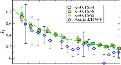
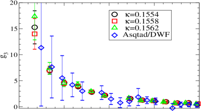
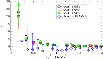
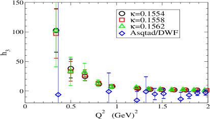
Figure 1: Results for the four axial form-factors, $g_{1}$, $g_{3}$, $h_{1}$ and $h_{3}$. The dashed curve shows consistency of $g_{1}$ for the $\kappa=0.1562$ ensemble with a dipole fit giving a pole mass of $1.67(5)$GeV.

5 Effective couplings

Referring to Eq. (3), we decompose the $\Delta$ matrix elements of the pseudoscalar current into two axial $\pi\Delta\Delta$ couplings, $G_{\pi\Delta\Delta}$ and $H_{\pi\Delta\Delta}$, with the relation:

$$2m_{q}\langle\Delta_{p_{f}}|P|\Delta_{p_{i}}\rangle\equiv\left(\frac{m_{\Delta}^{2}}{E_{\Delta}(\vec{p}_{f})E_{\Delta}(\vec{p}_{i})}\right)\frac{2f_{\pi}m_{\pi}^{2}}{(m_{\pi}^{2}-q^{2})}\left[g^{\alpha\beta}G_{\pi\Delta\Delta}(q^{2})+\frac{q^{\alpha}q^{\beta}}{4m_{\Delta}^{2}}H_{\pi\Delta\Delta}(q^{2})\right]\overline{u}_{\alpha}\gamma^{5}u_{\beta}$$ (16)

and we identify:

$$m_{q}\tilde{g}\equiv\frac{f_{\pi}m_{\pi}^{2}G_{\pi\Delta\Delta}(q^{2})}{(m_{\pi}^{2}-q^{2})}\qquad{\rm and}\qquad m_{q}\tilde{h}\equiv\frac{f_{\pi}m_{\pi}^{2}H_{\pi\Delta\Delta}(q^{2})}{(m_{\pi}^{2}-q^{2})}$$ (17)

Note that because the two different possible contractions of the Dirac indices of the $3/2$-spinors give us two pseudoscalar form-factors we get two effective axial couplings, unlike the case of the nucleon and the $N-\Delta$ transition. The quark mass $m_{q}$ is computed from the axial Ward-Takahashi identity and $f_{\pi}$ from the pion-to-vacuum amplitude. Both are computed from appropriate combinations of two-point functions as shown in the reference [3]. The renormalization factor $Z_{P}$ is not required as its occurrences in $m_{q}$ and $\tilde{g}$ or $\tilde{h}$ cancel.

The results for these form-factors are shown in Fig. 2. As can be seen, despite the large statistical errors, $G_{\pi\Delta\Delta}$ increases with decreasing $Q^{2}$ for the unquenched lattices.

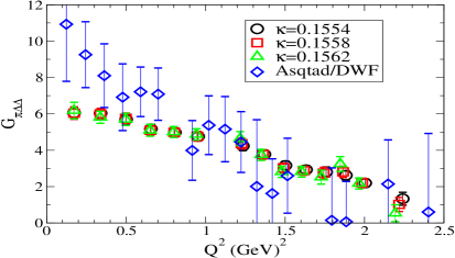
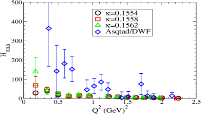
Figure 2: The effective couplings $G_{\pi\Delta\Delta}$ and $H_{\pi\Delta\Delta}$ for the quenched ensemble with $\kappa=0.1554$.

6 Goldberger-Treiman relations

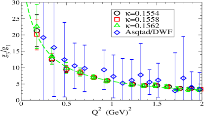
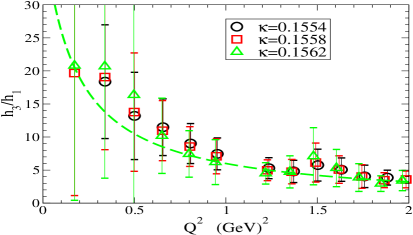
Figure 3: Ratios of axial form-factors, $g_{3}/g_{1}$ and $h_{3}/h_{1}$. Dashed curves show consistency with a pion pole fit for the $\kappa=0.1562$ ensemble. We omit the mixed ensemble from the $h_{3}/h_{1}$ plot as the signal is washed out by the larger error bars.

From the axial Ward-Takahashi identity, we have the relationship

$$\langle\Delta|\partial_{\mu}A^{\mu}|\Delta\rangle=2m_{q}\langle\Delta|P|\Delta\rangle.$$ (18)

Applying the momentum operator on (1) and (2), the left-hand side gives

$$\langle\Delta|\partial_{\mu}A^{\mu}|\Delta\rangle=2m_{\Delta}\left[(g_{1}-\tau g_{3})g^{\alpha\beta}+(h_{1}-\tau h_{3})\frac{q^{\alpha}q^{\beta}}{4m_{\Delta}^{2}}\right]\overline{u}_{\alpha}\gamma^{5}u_{\beta}$$ (19)

with $\tau=\frac{-q^{2}}{(2m_{\Delta})^{2}}$. Using Eqs. (16) we get

$$2m_{\Delta}\left(g_{1}-\tau g_{3}\right)=\frac{2f_{\pi}m_{\pi}^{2}G_{\pi\Delta\Delta}(q^{2})}{(m_{\pi}^{2}-q^{2})}\qquad{\rm and}\qquad 2m_{\Delta}\left(h_{1}-\tau h_{3}\right)=\frac{2f_{\pi}m_{\pi}^{2}H_{\pi\Delta\Delta}(q^{2})}{(m_{\pi}^{2}-q^{2})}.$$ (20)

If we demand that the $g_{3}$ and $h_{3}$ terms cancel the pole at $q^{2}=m_{\pi}^{2}$, we get the Goldberger-Treiman relations. In Figure 3 we show that the ratios $g_{3}/g_{1}$ and $h_{3}/h_{1}$ are consistent with pion-pole behavior. We note that, as with the effective axial couplings, there are two Goldberger-Treiman relations, namely:

$$f_{\pi}G_{\pi\Delta\Delta}(q^{2})=m_{\Delta}g_{1}(q^{2})\qquad{\rm and}\qquad f_{\pi}H_{\pi\Delta\Delta}(q^{2})=m_{\Delta}h_{1}(q^{2}).$$

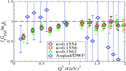
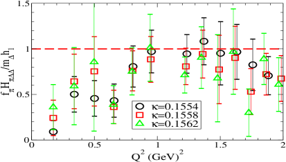
Figure 4: The two Goldberger-Treiman relations for the $\Delta$ baryon.

In Fig. 4 we plot the ratio of the left-hand to right-hand sides of the expressions given in (6). For low $Q^{2}$, these quenched ratios deviate from unity but are in agreement with unity for $Q^{2}\stackrel{{\scriptstyle>}}{{\sim}}0.8{\rm GeV}^{2}$. Similar behavior was observed for $G_{\pi NN}$ and $G_{\pi N\Delta}$ in [3]. In the unquenched ensemble the errors are too large to enable any conclusions.

7 Conclusions

In this work we have evaluated, for the first time, the $\Delta^{+}$ axial form factors, $g_{1}$, $g_{3}$, $h_{1}$, $h_{3}$ as well as the pseudoscalar form factors $\tilde{g}$, $\tilde{h}$. We have shown that these axial and pseudoscalar vertex compositions yield two effective $\pi\Delta\Delta$ couplings, $G_{\pi\Delta\Delta}$, and $H_{\pi\Delta\Delta}$, which in turn satisfy dual Goldberger-Treiman relations. Results obtained in the quenched theory are accurate enough to enable a check of these relations and show that there are deviations for small $Q^{2}$ values where chiral effects are expected to be large. Unquenched results using a mixed action have large statistical errors and require further analysis for allowing a definite conclusion to be reached.

References

- [1] C. Alexandrou et al., Phys. Rev. D 69, 114506 (2004). C. Alexandrou, et al., Phys. Rev. D 77, 085012 (2008). C. Alexandrou, et al., Phys. Rev. Lett. 94, 021601 (2005).
- [2] C. Alexandrou, G. Koutsou, J. W. Negele and A. Tsapalis, Phys. Rev. D 74, 034508 (2006).
- [3] C. Alexandrou et al., Phys.Rev. D 76,094511 (2007).
- [4] D. B. Leinweber, T. Draper and R. M. Woloshyn, Phys. Rev. D 46, 3067 (1992).
- [5] M. Kotulla et al., Phys. Rev. Lett. 89, 272001 (2002).
- [6] G. Lopez Castro and A. Mariano, Phys. Lett. B 517, 339 (2001).
- [7] C. Alexandrou et al., Nucl. Phys. A 825, 115 (2009).
- [8] C. W. Bernard et al., Phys. Rev. D 64, 054506 (2001).
- [9] T. Draper, PhD thesis, UCLA, 1984. D. Dolgov et al. , Phys. Rev. D 66, 034506 (2002).
- [10] F. J. Jiang and B. C. Tiburzi, Phys. Rev. D 78, 017504 (2008).
- [11] K. Nakamura et al. (Particle Data Group), J. Phys. G 37, 075021 (2010).