Optimal excitation of two dimensional Holmboe instabilities

Abstract

(Under consideration for publication in Physics of Fluids.)
(Submitted on 27 Oct 2010 (v1), last revised 14 Apr 2011 (this version, v2))

Highly stratified shear layers are rendered unstable even at high stratifications by Holmboe instabilities when the density stratification is concentrated in a small region of the shear layer. These instabilities may cause mixing in highly stratified environments. However these instabilities occur in limited bands in the parameter space. We perform Generalized Stability analysis of the two dimensional perturbation dynamics of an inviscid Boussinesq stratified shear layer and show that Holmboe instabilities at high Richardson numbers can be excited by their adjoints at amplitudes that are orders of magnitude larger than by introducing initially the unstable mode itself. We also determine the optimal growth that is obtained for parameters for which there is no instability. We find that there is potential for large transient growth regardless of whether the background flow is exponentially stable or not and that the characteristic structure of the Holmboe instability asymptotically emerges as a persistent quasi-mode for parameter values for which the flow is stable.

I Introduction

The mixing of shear layers and the development of turbulence is severely impeded when the layer is located in regions of large stable stratification. The stratification is usually quantified with the non-dimensional Richardson number defined as the ratio of the local Brunt-Väisälä frequency $N^{2}$ to the square of the local shear $U^{\prime}$, $\text{Ri}=N^{2}/U^{\prime 2}$. Large stratification corresponds to large Richardson numbers. The significance of the Richardson number for the stability of stratified flows has been underscored with a theorem due to Miles and Howard Miles (1961); Howard (1961) which proves that if everywhere in the flow $\text{Ri}>1/4$, the flow is necessarily stable to exponential instability. The essential instability that leads primarily to mixing in both stratified and unstratified shear layers is the Kelvin-Helmholtz (KH) instability Drazin and Reid (1981). The KH modes are eventually stabilized when the local Richardson number exceeds $1/4$, but if the stratification is concentrated in narrow regions within the shear layer the Richardson number may locally become smaller than $1/4$ and an instability can result although the overall stratification is very large. Under such conditions, a new branch of instability of stratified shear layers emerges as shown by Holmboe Holmboe (1962), consisting of a pair of propagating waves with respect to the center flow, one prograde and one retrograde. This new instability branch has been named the Holmboe (H) instability and it is physically very interesting because it persists at all stratifications and can lead to mixing in highly stratified shear layers.

Holmboe instabilities have been reproduced in laboratory experiments Thorpe (1971); Browand and Winant (1973); Pouliquen et al. (1994); Caulfield et al. (1995); Zhu and Lawrence (2001); Hogg and Ivey (2003); Tedford et al. (2009) and have been numerically simulated Smyth et al. (1988); Sutherland et al. (1994); Smyth (2006); Smyth and Peltier (2006); Smyth et al. (2007); Carpenter et al. (2007); Alexakis (2009); Tedford (2009). At finite amplitude these Holmboe modes equilibrate into propagating waves and they can induce mixing in highly stratified environments Smyth et al. (1988); Smyth and Winters (2003); Carpenter et al. (2007). Consequently, Holmboe instabilities present the intriguing possibility that they may be responsible for transition to turbulence and mixing in highly stratified flows. In that vein, Alexakis Alexakis (2005, 2007, 2009) has proposed that the surmised necessary mixing in order for a thermonuclear runway to occur and highly stratified white dwarfs form supernova explosions could be effected with Holmboe instabilities.

Holmboe Holmboe (1962) also introduced a new method for analyzing the perplexing instabilities that may arise with the introduction of stratification. He went beyond classical modal analysis and proposed that a fruitful program for predicting and obtaining a clear physical idea of the instability of stratified shear flows is to simplify the background flow to segments of piecewise constant vorticity, as in Rayleigh’s seminal work Rayleigh (1880), and then consider the dynamics of the edge waves that are supported at each vorticity and density discontinuity. Holmboe showed that the flow becomes unstable when the edge waves propagate with the same phase speed. This method of analysis has been extended and used to clarify the detailed mechanism of instability in stratified flows Baines and Mitsudera (1994); Caulfield (1994); Haigh and Lawrence (1999); Harnik et al. (2008); Rabinovich et al. (2011) and has been shown recently by Carpenter et al. Carpenter et al. (2010) to be capable of readily assessing the character of instability of non-idealized observed flows. Also this edge wave description has elucidated the dynamics of other instabilities that occur in geophysics Bretherton (1966); Sakai (1989); Heifetz and Methven (2005); Bakas and Ioannou (2009) and astrophysics  Goldreich et al. (1986); Narayan et al. (1987); Umurhan (2010).

However, the efficacy of Holmboe modes to mix highly stratified layers can be questioned because the instability occurs only in limited regions of parameter space and the modal growth rate of the instability becomes exponentially small with stratification. Specific estimates of the asymptotic behavior of the growth rates and of the unstable band of wavenumbers has been recently obtained by Alexakis Alexakis (2007). Also the introduction of viscosity can further reduce the growth rates of the Holmboe instabilities. It is the purpose of this work to go beyond the modal analysis and investigate the non-modal stability of stratified shear layers that are Holmboe unstable in order to assess the true potential of growth of stratified shear layers. We will achieve this using the standard methods of generalized stability theory Farrell and Ioannou (1996); Schmid and Henningson (2001).

Because shear layers are powerful transient amplifiers of perturbation energy, we expect that the Holmboe instabilities can be excited at enhanced amplitude by composite non-modal perturbations. Even in the case of an infinite constant shear flow which has a continuous spectrum with no inviscid analytic modes and all perturbations eventually decay algebraically with time, the non-modal solutions constructed by Kelvin Kelvin (1887) demonstrate that the asymptotic limit is non-uniform and perturbation energy can transiently exceed any chosen bound in the inviscid limit; the same is true for bounded Couette flow as shown by Orr Orr (1907). The Kelvin-Orr solutions can be extended to stratified flows Phillips (1966); Hartmann (1975) and these solutions can produce transient perturbation growth that can also exceed in the inviscid limit any bound Farrell and Ioannou (1993a). Specifically it can be shown that in constant shear flow and large Richardson numbers the perturbation energy amplification is the square root of that achieved in the absence of stratification. The same robust growth resulting from the continuous spectrum is expected to persist in all shear layers as the dynamics of the Orr waves are universal and do not depend on the details of the background shear flow Farrell and Ioannou (1993b).

Furthermore in shear layers of finite size the vorticity and density edge waves that are concentrated in regions of vorticity and density discontinuities can interact and produce transient perturbation growth Heifetz et al. (1999). Also the transiently growing Kelvin-Orr vorticity structures may deposit their energy to the edge waves Bakas and Ioannou (2009) or to propagating gravity waves Lott (1997); Bakas and Ioannou (2007); Lott et al. (2010). In general the continuous spectrum can excite at high amplitude the unstable or even stable analytic modes Farrell (1988a, 1989) and maintain under continuous excitation high levels of variance in stable flows Farrell and Ioannou (1993c); Farrell and Ioannou (1994).

In this work we will consider the generalized stability of a Boussinesq stratified shear layer. The Boussinesq approximation makes inaccurate predictions of the dispersion relation of the perturbations in the shear layers when the stratification is locally very large Umurhan and Heifetz (2007). However we have found that the resulting optimal growths are not sensitive to this approximation and in this paper in order to make contact with previous work we will only present results obtained using the Boussinesq approximation. Also following Hazel Hazel (1972) and the work of Smyth and Peltier Smyth and Peltier (1989, 1990) we will consider a continuous version of Holmboe’s velocity profile with the characteristic density stratification embedded in the shear layer. Hazel and Smyth and Peltier had analyzed the character of the bifurcations that occur in the instability of the continuous profile as the Richardson number at the center of the shear layer increases. Alexakis Alexakis (2005, 2007, 2009) extended the analysis to even higher stratifications and was able to predict theoretically and show numerically that there are higher branches of Holmboe instabilities in these continuous profiles. Because of the geophysical and astrophysical interest we will concentrate our analysis of non-modal perturbation growth of shear layers at very high Richardson numbers which possess sparse islands of exponential instability of low growth rate.

II Formulation

We will study the stability of an inviscid, unidirectional, stratified, step like channel flow to two dimensional incompressible perturbations. The mean flow is characterized by a velocity jump $\Delta U$ over a vertical scale $h_{0}$ and the associated statically stable mean density is characterized by a density jump $\Delta\rho$. The linearized nondimensional perturbation equations about the mean flow $U_{0}(z)$ and mean density $\rho_{0}(z)$ in the Boussinesq approximation are:

$$\left(\partial_{t}+U_{0}\partial_{x}\right)u =-U_{0}^{\prime}\,w-\partial_{x}p$$ (1a)

$$\left(\partial_{t}+U_{0}\partial_{x}\right)w =-J\varrho-\partial_{z}p$$ (1b)

$$\left(\partial_{t}+U_{0}\partial_{x}\right)\varrho =-\rho_{0}^{\prime}\,w$$ (1c)

$$\partial_{x}u+\partial_{z}w =0$$ (1d)

The density of the fluid has been decomposed as: $\rho\equiv\rho_{m}+\rho_{0}(z)+\varrho(x,z,t)$, where $\rho_{m}$ is the mean background density, $\rho_{0}(z)$ is the mean density variation and $\varrho(x,z,t)$ is the perturbation density; and furthermore, according to the Boussinesq approximation, we assume, $|\rho_{0}|\ll\rho_{m}$ and $|\varrho|\ll\rho_{m}$. We denote with $u$ and $w$ the perturbation velocities in the streamwise ($x$) and vertical ($z$) direction and $p$ is the perturbation reduced pressure. Differentiation with respect to $z$ is denoted with a dash. The perturbation equations have been made nondimensional, choosing $h_{0}$ as the length scale, $\Delta U$ as the velocity scale, and $\Delta\rho$ as the scale for the density. Time has been scaled with $h_{0}/\Delta U$, and pressure has been scaled with $\rho_{m}\left(\Delta U\right)^{2}$. The local Richardson number is

$$\text{Ri}=-J\frac{\rho_{0}^{\prime}}{U_{0}^{\prime 2}}$$ (2)

with

$$J=\frac{g\,\Delta\rho\,h_{0}}{\rho_{m}\,\Delta U^{2}}~{}.$$ (3)

$J$ provides a measure of the bulk Richardson number of the shear layer. We will assume that the flow is in a channel of length $L=2h_{0}$ and impose at the channel boundaries zero vertical velocity, $w$, and zero perturbation density, $\varrho$. The length of the channel has been selected so that boundaries do not affect in an important way the results that we report in this paper. We have checked by doubling the channel size that the eigenspectrum and the perturbation transient growth are converged. Similar insensitivity to the location of the channel walls has been previously reported by Alexakis Alexakis (2009).

The perturbation equations can be written compactly by introducing a streamfunction $\psi$ so that the velocities are $u=\partial_{z}\psi$ and $w=-\partial_{x}\psi$, and the vertical displacement, defined through the relation:

$$\left(\partial_{t}+U_{0}\partial_{x}\right)\eta=w~{},$$ (4)

can replace the perturbation density as:

$$\varrho=-\rho_{0}^{\prime}\,\eta~{}.$$ (5)

The perturbation state will be determined by the fields $\psi$ and $\eta$. Because of homogeneity in the streamwise direction, the perturbation state can be decomposed in Fourier components in $x$:

$$\hat{{\bf x}}(z,t)e^{ikx}=[\hat{\psi}(z,t),\hat{\eta}(z,t)]^{\text{T}}e^{ikx}$$ (6)

and the perturbation dynamics for the Fourier amplitudes for each wavenumber $k$ can be written compactly in the form:

$$\frac{\partial\,\hat{{\bf x}}}{\partial t}=\mathbb{A}\,\hat{{\bf x}}~{},$$ (7)

with the operator $\mathbb{A}$ given by:

$$\mathbb{A}=-ik\left[\begin{array}[]{cc}\Delta^{-1}\left(U_{0}\Delta-U_{0}^{\prime\prime}\right){}{}{}{}{}&J\Delta^{-1}\rho_{0}^{\prime}\\ 1&U_{0}\end{array}\right]~{}.$$ (8)

With $\Delta=\partial_{zz}^{2}-k^{2}$ we denote the two dimensional Laplacian for the $k$ streamwise wavenumber. $\Delta^{-1}$ is the inverse Laplacian, the inversion being rendered possible and unique by imposing the boundary conditions on the upper and lower boundaries. The perturbation equation (7) is equivalent to the time dependent Taylor-Goldstein equation:

$$\left(\partial_{t}+ikU_{0}\right)^{2}\Delta\hat{\psi}-ikU_{0}^{\prime\prime}\left(\partial_{t}+ikU_{0}\right)\hat{\psi}+k^{2}J\rho_{0}^{\prime}\hat{\psi}=0~{}.$$ (9)

III Kelvin-Helmholtz and Holmboe instabilities of a shear layer

Following Hazel Hazel (1972), we consider the following background mean velocity and density:

$$U_{0}(z)=\frac{1}{2}\tanh{\left(2z\right)}~{}~{},~{}~{}\rho_{0}(z)=-\frac{1}{2}\tanh{\left(2Rz\right)}~{}.$$ (10)

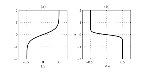
Figure 1: (a): Mean velocity profile as a function of height. (b): Mean density profile as a function of height for $R=3$.

The mean velocity and density profiles are shown in FIG. 1 for $R=3$. The parameter $R$ is the ratio of the width of the shear layer to the width of the region over which the density jump occurs. The local Richardson number is given by,

$$\text{Ri}(z)=RJ\frac{\mathop{\mathrm{sech}}^{2}{\left(2Rz\right)}}{\mathop{\mathrm{sech}}^{4}{\left(2z\right)}}~{}.$$ (11)

The Richardson number at the center is related to the bulk Richardson number through the relation:

$$\text{Ri}(0)=RJ~{}.$$ (12)

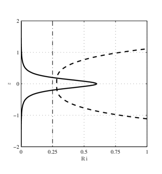
Figure 2: Richardson number as a function of height for the velocity and density profiles in FIG. 1 for $J=0.2$ and $R=3$ (solid). The Richardson number assumes values smaller than $1/4$ away from the center and the flow may be exponentially unstable. Also shown is the case of $J=0.2$, $R=\sqrt{2}$ (dashed). In this case the Richardson number is everywhere greater than $1/4$ and the velocity profile is by necessity exponentially stable. The threshold value $\text{Ri}=1/4$ (dash-dot) is also indicated.

When $R=1$ the local Richardson number assumes its minimum value at the center, $\text{Ri}(0)=RJ$, and the shear layer is unstable only if $\text{Ri}(0)<1/4$. The instability that results is a Kelvin-Helmholtz (KH) type instability with a short wave cutoff and zero phase velocity. For $R>2$ the Richardson number decays exponentially to zero. This exponential decay allows the local Richardson number to be in regions smaller than $1/4$ and the shear layer may become unstable although both the bulk stratification $J$ and $\text{Ri}(0)$ may be very large. The instabilities that occur under these conditions are the Holmboe instabilities (H). The variation of the Richardson number with height is shown in FIG. 2 for $R=3$, a case that supports Holmboe instabilities and will be treated in detail in this paper, and for $R=\sqrt{2}$ which can support only KH instability when the Richardson number at the center is smaller than $1/4$.

In order to determine the modal stability of the velocity and density profiles (10) we assume modal solutions of (7) of the form $\hat{{\bf x}}(z,t)=[\hat{\psi}_{c}(z),\hat{\eta}_{c}(z)]^{\text{T}}e^{-ikct}$, with $-ikc$ an eigenvalue of the evolution operator $\mathbb{A}$ in (8). The modal growth rate of the perturbation is $kc_{i}$ where $c_{i}=\Im(c)$ and the flow is exponentially unstable to perturbations of wavenumber $k$ if $c_{i}>0$. The real part, $c_{r}$, of the eigenvalue $c(k)$, gives the phase speed of the perturbation. Detailed analysis of the eigenspectrum of (10) and the bifurcation from KH instabilities to H instabilities has been already performed Hazel (1972); Smyth and Peltier (1989, 1990); Alexakis (2005, 2007, 2009). Here we review the basic stability characteristics for the case of $R=3$ that admits both KH and H instability modes.

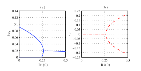
Figure 3: (Color online) Bifurcation properties of the unstable modes as a function of the Richardson number at the center of the shear zone $\text{Ri}(0)=RJ$ for the mean state (10) for $R=3$ and perturbations with $k=0.3$. (a) the growth rate $kc_{i}$ (solid); (b) the associated phase speed $c_{r}$ (dashed-dot). For $\text{Ri}(0)<0.242$ there is a single Kelvin-Helmholtz (KH) mode with zero phase speed. For $0.242<\text{Ri}(0)<0.258$ there are two KH modes with zero phase speed. The two KH modes coalesce to produce two unstable Holmboe (H) modes with equal and opposite phase speeds.

The transition from KH instability to H instability is shown in FIG. 3 where we plot the growth rate and phase speed as a function of the Richardson number at the center of the shear zone $\text{Ri}(0)$ for $k=0.3$. For $\text{Ri}(0)<0.242$, there is a single unstable Kelvin-Helmholtz instability with phase speed $c_{r}=0$. At $\text{Ri}(0)=0.242$ a second KH mode becomes unstable, also with $c_{r}=0$. The KH modes coalesce at $\text{Ri}(0)=0.258$ to form a propagating pair of unstable Holmboe modes with equal and opposite phase speeds and the same growth rate. In this case we see two branches of KH instabilities existing even when the center Richardson number exceeds $1/4$ (the Richardson number assumes values smaller than $1/4$ way from the center because the parameter is $R=3$, see FIG. 2); a similar case can be found in Smyth and Peltier Smyth and Peltier (1989).

Numerical results were obtained by discretizing the channel and all differential operators using second order centered differences and incorporating the appropriate boundary conditions. Equation (7) then becomes a matrix equation in which the state becomes a column vector. We used a staggered grid, that is, we evaluated $\hat{\psi}_{c}(z)$ at $N$ interior points in the vertical and $\hat{\eta}_{c}(z)$ at $N+1$ points located halfway between the collocation points of the streamfunction. The eigenspectrum is obtained by eigenanalysis of operator $\mathbb{A}$. Calculations, unless otherwise specified, were performed with $N=1001$ in the domain $-2\leq z\leq 2$. With this discretization the finite time evolution of the dynamics is well resolved when there is no instability up to a time of $t=O(1/(\alpha k\Delta z))$ where $\alpha$ is the typical shearFarrell and Ioannou (1993a). However, in order to numerically resolve the curves of zero modal growth of the Holmboe modes of instability we had to include numerical diffusion in both the momentum and density equations with coefficient of diffusion $\nu=(\Delta z/2)^{2}$ in the momentum equation and $\nu/9$ in the density equation for the case $R=3$ ($\Delta z$ is the grid spacing). Very accurate determination of the neutral curve in the inviscid limit can be obtained, using the shooting method as in Alexakis Alexakis (2007).

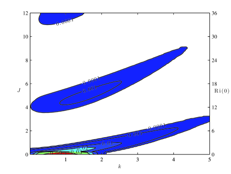
Figure 4: (Color online) Contours of modal growth rate $kc_{i}$ of the perturbation operator $\mathbb{A}$ as a function of wavenumber, $k$, and the bulk Richardson number, $J$, for $R=3$. Because of the inclusion of diffusion the instability bands do not extend to infinity as the do in the inviscid limit. The corresponding value of the Richardson number at the origin $\text{Ri}(0)=RJ$ is also recorded at the ordinate axis on the right. For this value of $R$ there are KH unstable modes with phase speed $c_{r}=0$ for small values of $J$ (barely discernible in this plot) and three unstable bands of pairs of H instabilities with prograde and retrograde phase speeds for higher $J$.

Growth rate contours as a function of stratification, $J$ or $\text{Ri}(0)$, and wavenumber, $k$ are shown in FIG. 4 for $R=3$. The region of KH instability is concentrated for small Richardson numbers and it is not discernible in this plot. However the bands of instability corresponding to the various Holmboe modes of instability can be clearly seen. Note that because of the inclusion of diffusion the instability bands do not extend to infinity as they do in the inviscid limit Holmboe (1962); Howard and Maslowe (1973); Baines and Mitsudera (1994); Alexakis (2005).

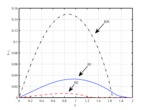
Figure 5: (Color online) Growth rates $kc_{i}$ as a function of wavenumber $k$ for: a KH instability for $\text{Ri}(0)=0.06$ (dash-dot), an H1 mode of instability for $\text{Ri}(0)=0.65$ (solid) and an H2 mode of instability for $\text{Ri}(0)=12$ (dashed). The growth rates of H2 mode have been multiplied by 10.

The first band in FIG. 4 is the first Holmboe mode of instability, H1, (for $J>0.0833$), the second is the second Holmboe instability mode, H2, (for $J>3.5$) and we can also partly see the growth rate of the third Holmboe instability mode, H3 (for $J>10$). Estimates of the growth rates of these higher modes and regions of instability can be found in Alexakis Alexakis (2007) who shows that the growth rate of the Holmboe instabilities is decreasing exponentially with stratification and as the Holmboe modes approach neutrality the critical layer of the instabilities, that is the height $z_{c}$ for which $U_{0}(z_{c})=c_{r}$, tends to the height that corresponds to the maximum/minimum velocity $\pm 0.5$ of the shear zone Alexakis (2007). We obtain a sense of the ordering of the growth rates of the KH and H instabilities in FIG. 5. In that figure we plot the modal growth rates $kc_{i}$ as a function of wavenumber $k$ for $R=3$ and center Richardson numbers $\text{Ri}(0)=0.06,\ 0.65,\ 12$ for which we have respectively KH mode instability, H1 and H2 instabilities.

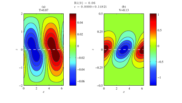
Figure 6: (Color online) Structure of the streamfunction (panel (a)) and density (panel (b)) perturbation fields of an unstable KH mode with growth rate $kc_{i}=0.1482$ and phase speed $c_{r}=0$. Critical layer at $z_{c}=0$ (dashed). For perturbations with $k=1$, and base flow with $R=3$ and $\text{Ri}(0)=0.06$.

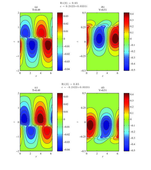
Figure 7: (Color online) Structure of the streamfunction and density perturbation fields of unstable H1 modes with growth rate $kc_{i}=0.0331$ and phase speeds $c_{r}=\pm 0.2423$. Panels (a) and (b): streamfunction and density contours for the prograde H1 mode. Panels (c) and (d): for the retrograde H1 mode. Critical layer at $z_{c}=\pm 0.264$ (dashed). For perturbations with $k=1$, and base flow with $R=3$ and $\text{Ri}(0)=0.65$.

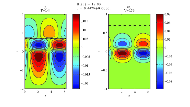
Figure 8: (Color online) Structure of the streamfunction (panel (a)) and density (panel (b)) perturbation fields of unstable prograde H2 mode with growth rate $kc_{i}=0.0006$ and phase speed $c_{r}=0.4425$. Critical layer at $z_{c}=0.698$ (dashed). For perturbations with $k=1$, and base flow with $R=3$ and $\text{Ri}(0)=12.00$.

Typical structure of the KH instability mode is shown in FIG. 6 for $k=1$, $R=3$ and $\text{Ri}(0)=0.06$. For these parameters the coalescence of the KH modes and the emergence of the first Holmboe mode of instability occurs at $\text{Ri}(0)=0.182$. The Holmboe modes come in prograde and retrograde pairs. The prograde and retrograde unstable Holmboe modes, H1, for $\text{Ri}(0)=0.65$ are shown in FIG. 7. Because they are symmetric with respect to $z=0$, we will subsequently plot only the prograde branch of the H mode. Higher Holmboe modes have larger vertical wavenumbers, the case of H2 is shown in FIG. 8. In the idealized piecewise constant problem studied by Holmboe (see Appendix A) the prograde Holmboe instability arises from resonant interaction between the edge waves at the density discontinuity at the center with the edge wave at the upper vorticity discontinuity, and with the edge wave at the lower vorticity discontinuity for the retrograde instabilityBaines and Mitsudera (1994). The same type of interaction gives rise to the Holmboe instability modes when the discontinuities of the background are smoothed as for the background given by Eq. (10). Because of the delta function nature of the vorticity and stratification gradient the edge waves in Holmboe’s idealized profile do not have internal structure and as a result there is a single pair of unstable Holmboe instabilities that can arise from the interaction. The smoothed profile allows the edge wave to obtain vertical structure within the regions of large vorticity and stratification gradient (cf. respectively to the left and right panels of FIG. 7 and FIG. 8) and the H2, H3, etc Holmboe instabilities emerge, with the higher modes associated with higher vertical wavenumber structure.

IV Optimal excitation of Kelvin-Helmholtz and Holmboe modes

The perturbation dynamics in a stratified shear flow are non-normal and, as we will show in this section, the unstable modes emerge through excitation of their adjoint. In order to determine the growth that results by introducing initially the adjoint of the unstable mode we derive the adjoint perturbation dynamics in the energy norm. For a perturbation of wavenumber $k$ the total average kinetic energy over a wavelength in the region $[z_{1},z_{2}]$ is:

$$T=\frac{1}{4}\int\limits_{z_{1}}^{z_{2}}\!\text{d}z\;\hat{\psi}^{*}\left(-\Delta\hat{\psi}\right)~{},$$ (13)

and the potential energy is:

$$V=\frac{1}{4}\int\limits_{z_{1}}^{z_{2}}\!\text{d}z\;J\left(-\rho_{0}^{\prime}\right)\hat{\eta}^{*}\hat{\eta}~{},$$ (14)

The total energy of a perturbation $\hat{{\bf x}}=[\hat{\psi},\hat{\eta}]^{\text{T}}$ is thus given by the inner product:

$$||\hat{{\bf x}}||^{2}=(\hat{{\bf x}},\hat{{\bf x}})=\frac{1}{4}\int_{z_{1}}^{z_{2}}\text{d}z\;\left[\hat{\psi}^{*}\,\left(-\Delta\hat{\psi}\right)+J\left(-\rho_{0}^{\prime}\right)\hat{\eta}^{*}\hat{\eta}\right]~{}.$$ (15)

The adjoint operator $\mathbb{A}^{\dagger}$ in this inner product is defined as the operator that satisfies:

$$\left(\vphantom{\dot{W}}\mathbb{A}^{\dagger}\hat{\mathbf{f}}_{\alpha},\hat{\mathbf{g}}\right)=\left(\vphantom{\dot{W}}\hat{\mathbf{f}}_{\alpha},\mathbb{A}\,\hat{\mathbf{g}}\right)~{},$$ (16)

for any two states $\hat{\mathbf{f}}_{\alpha}=[\hat{\psi}_{\alpha},\hat{\eta}_{\alpha}]^{\text{T}}$ and $\hat{\mathbf{g}}=[\hat{\psi},\hat{\eta}]^{\text{T}}$. For a discussion of the adjoint equation in fluid mechanics see Farrell Farrell (1988b), Hill Hill (1995), Farrell and Ioannou Farrell and Ioannou (1996), Chomaz et. al. Marquet et al. (2009) and Schmid and Henningson Schmid and Henningson (2001).

From (16) the adjoint operator of (8) in the energy inner product is easily shown to be:

$$\mathbb{A}^{\dagger}=ik\left[\begin{array}[]{cc}\Delta^{-1}\left(U_{0}\Delta+2U_{0}^{\prime}\,\text{D}\right){}{}{}{}{}&J\Delta^{-1}\rho_{0}^{\prime}\\ 1&U_{0}\end{array}\right]~{},$$ (17)

with $\text{D}=\text{d}/\text{d}z$ denoting differentiation with respect to $z$, and the adjoint evolution equation is

$$\frac{\partial\hat{{\bf x}}_{\alpha}}{\partial t}=\mathbb{A}^{\dagger}\,\hat{{\bf x}}_{\alpha}$$ (18)

with the adjoint boundary conditions $\hat{{\bf x}}_{\alpha}(z_{i},t)=0$ at the channel walls $z_{i}$. This equation produces the adjoint of the time-dependent Taylor-Goldstein equation  (9):

$$\left(\partial_{t}-ikU_{0}\right)^{2}\Delta\hat{\psi}_{\alpha}-2ikU_{0}^{\prime}\left(\partial_{t}-ikU_{0}\right)\text{D}\hat{\psi}_{\alpha}-k^{2}J\rho_{0}^{\prime}\hat{\psi}_{\alpha}=0~{}.$$ (19)

The eigenvalues of the adjoint operator $\mathbb{A}^{\dagger}$ are the complex conjugate of the eigenvalues of $\mathbb{A}$ and in this way we can establish a correspondence between the modes of the adjoint $\mathbb{A}^{\dagger}$ and the modes of $\mathbb{A}$. Further, the mode of the adjoint with eigenvalue $ikc^{*}$, $\hat{{\bf x}}_{\alpha\,c}$, and the mode of $\mathbb{A}$ with eigenvalue $-ikc^{\prime}$, $\hat{{\bf x}}_{c^{\prime}}$, satisfy the biorthogonality relation:

$$\left(\vphantom{\dot{W}}\hat{{\bf x}}_{\alpha\,c},\hat{{\bf x}}_{c^{\prime}}\right)=0\quad\text{for}\quad c\neq c^{\prime}~{}.$$ (20)

From (19) it can be verified that for any analytic mode of the Taylor-Goldstein equation  (9) with eigenvalue $-ikc$ (with $c_{i}>0$ or with $c_{r}$ outside the range of the background flow) the mode of $\mathbb{A}^{\dagger}$ with eigenvalue $ikc^{*}$ is:

$$\hat{{\bf x}}_{\alpha\,c}=\left[\begin{array}[]{c}\dfrac{\hat{\psi}_{c}^{*}}{U_{0}-c^{*}}\\ \dfrac{\hat{\eta}_{c}^{*}}{U_{0}-c^{*}}\end{array}\right]~{}.$$ (21)

From the biorthogonality relation (20) arises the physical importance of the modes of the adjoint: of all perturbations of unit energy the largest projection on a given mode is achieved by the adjoint of the mode. Indeed, a state written as a superposition of the modes of $\mathbb{A}$:

$$\hat{{\bf x}}=\sum_{c}a_{c}\,\hat{{\bf x}}_{c}~{},$$ (22)

will have coefficients $a_{c}$ given by:

$$a_{c}=\frac{\left(\hat{{\bf x}}_{\alpha\,c},\hat{{\bf x}}\right)}{(\hat{{\bf x}}_{\alpha\,c},\hat{{\bf x}}_{c})}~{}.$$ (23)

Because $|\left(\hat{{\bf x}}_{\alpha\,c},\hat{{\bf x}}\right)|\leq 1$, if the mode and the state $\hat{\bf x}$ are normalized, with equality when $\hat{{\bf x}}$ and $\hat{{\bf x}}_{\alpha\,c}$ are multiple to each other, the coefficients satisfy the inequality:

$$|a_{c}|\leq\frac{1}{|(\hat{{\bf x}}_{\alpha\,c},\hat{{\bf x}}_{c})|}~{},$$ (24)

and the maximum projection on a given mode is achieved by the adjoint mode, i.e. by choosing $\hat{{\bf x}}=\hat{{\bf x}}_{\alpha\,c}$. The adjoint perturbation excites the mode at an energy which is a factor

$$\frac{1}{|(\hat{{\bf x}}_{\alpha\,c},\hat{{\bf x}}_{c})|^{2}}~{},$$ (25)

greater than an initial condition consisting of the mode itself. For highly non-normal systems $|(\hat{{\bf x}}_{\alpha\,c},\hat{{\bf x}}_{c})|\ll 1$ and as a result this amplification may be very large, implying that the emergence of the mode in these systems is mainly due to the excitation of the adjoint. Although this is not a new result, it has not been noted in previous studies concerning Holmboe instabilities.

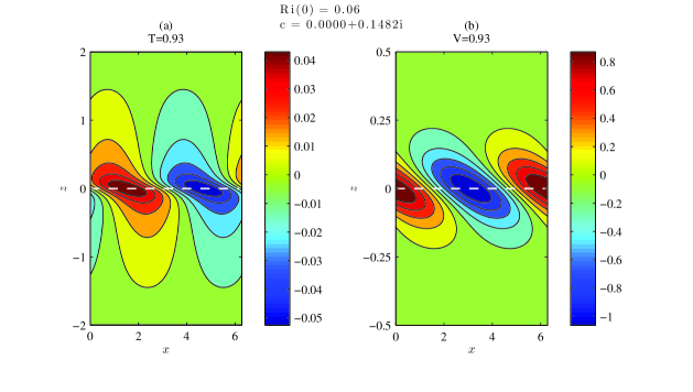
Figure 9: (Color online) Structure of the streamfunction (panel (a)) and density (panel (b)) perturbation fields of the adjoint of the unstable KH mode of FIG. 6. Parameters as in FIG. 6.

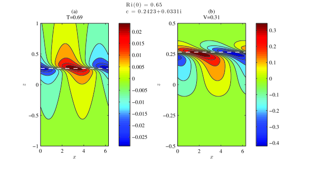
Figure 10: (Color online) Structure of the streamfunction and density perturbation fields of the adjoint of the unstable prograde H1 mode of FIG. 7. The adjoint is centered at the steering level, $z_{c}=0.264$, of the mode.

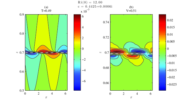
Figure 11: (Color online) Structure of the streamfunction and density perturbation fields of the adjoint of the unstable prograde H2 mode of FIG. 8. The adjoint is centered at the steering level, $z_{c}=0.698$, of the mode.

In FIG. 9 we plot the structure of the adjoint in the energy inner product of the unstable KH mode shown in FIG. 6 with $k=1$, $\text{Ri}(0)=0.06$ and $R=3$. An initial condition consisting of the adjoint of the most unstable mode excites the mode with energy 7.5 times greater than an initial condition consisting of the unstable mode itself. In FIGs. 10 and 11 we plot the adjoints of the two unstable Holmboe H1 and H2 modes, shown in FIGs. 7 and 8, both with the same $k=1$, $R=3$ and stratifications $\text{Ri}(0)=0.65$ and $\text{Ri}(0)=12$ respectively. The adjoints of the H1 and H2 modes are concentrated at the critical layer of the modes which is located way from the center of the shear layer and located in a region at the wings of the shear layer where the local Richardson number is less than $1/4$. An initial condition consisting of the adjoint of the H1 mode excites the most unstable mode with energy 69 greater than an initial condition consisting of the unstable mode itself. This energy amplification reaches 7921 for the excitation of the H2 mode by its adjoint.

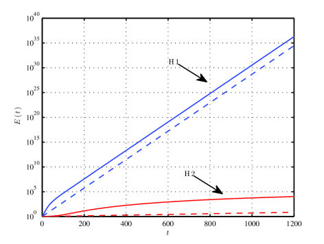
Figure 12: (Color online) Time evolution of the perturbation energy when the adjoint of the H1 mode shown in FIG. 10 and the H2 mode shown in FIG. 11 are introduced at $t=0$ (solid); also shown is the energy evolution if the H1 mode and H2 mode are introduced at $t=0$ (dashed). The adjoint excites the corresponding modes optimally. The adjoint of the H1 mode excites the mode at an amplitude a factor $69$ greater in energy than an initial condition consisting of the H1 mode itself. The H2 adjoint excites the mode at an amplitude a factor $7921$ greater in energy. Parameters are $k=1$, $R=3$ and for the H1 mode the stratification is $\text{Ri}(0)=0.65$, while for the H2 mode $\text{Ri}(0)=12$.

Initial conditions in the form of the adjoints of the most unstable mode evolve changing form and eventually assume the corresponding modal form. During their evolution, the adjoint perturbation extracts energy from the mean flow which is eventually deposited to the mode itself exciting it in this way at high amplitude. The time development of the energy of a unit energy initial condition in the form of the adjoints of the H1 and H2 mode is plotted in FIG. 12 demonstrating the increased excitation of the corresponding modes. This demonstrates that the unstable Holmboe modes at high Richardson numbers arise primarily due to excitation by their adjoint and the modal growth underestimates the growth of the instabilities.

V Optimal growth of perturbations and the emergence of the Holmboe quasi-mode

In the previous section we have demonstrated that for large Richardson numbers the adjoint of a mode can excite the modes at much higher amplitude. In this section we investigate the optimal growth of perturbations. The optimal growthFarrell (1988b); Farrell and Ioannou (1996); Schmid and Henningson (2001) of perturbations at time $t$ in the energy metric is obtained by calculating the norm of the propagator $e^{\mathbb{A}_{\mathbb{M}}t}$ where $\mathbb{A}_{\mathbb{M}}=\mathbb{M}^{1/2}\mathbb{A}\mathbb{M}^{-1/2}$ and $\mathbb{M}$ is the energy metric defined as

$$\mathbb{M}=\frac{\Delta z}{4}\left[\begin{array}[]{cc}-(\text{D}^{2}-k^{2})&0\\ 0&-J\rho_{0}^{\prime}\end{array}\right]~{},$$ (26)

so that total perturbation energy is given by $E=\hat{\bf x}^{\dagger}\mathbb{M}\hat{{\bf x}}$. The optimal growth is given by the largest singular value, $\sigma_{\max}$, of $e^{\mathbb{A}_{\mathbb{M}}t}$ and determines the largest perturbation growth that can be achieved at time $t$. The optimal perturbation, the initial perturbation that produces this growth, is $\hat{\bf x}_{\text{opt}}=\mathbb{M}^{-1/2}\mathbf{v}$, where $\mathbf{v}$ the right singular vector with singular value $\sigma_{\max}$.

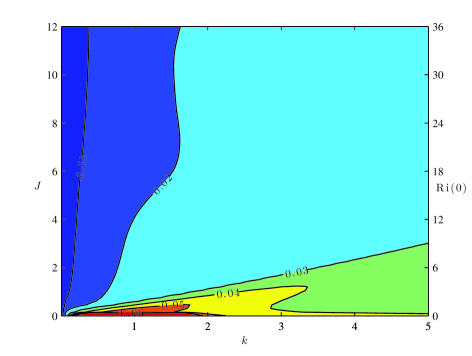
Figure 13: (Color online) Optimal growth for $t=100$. Contours of finite time Lyapunov exponent $\ln{\left(\sigma_{\max}(t)\right)}/t$ for $t=100$ as a function of wavenumber, $k$, and the bulk Richardson number, $J$, for $R=3$. The corresponding value of the Richardson number at the origin $\text{Ri}(0)=RJ$ is indicated at the ordinate axis on the right.

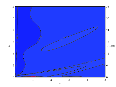
Figure 14: (Color online) Optimal growth for $t=600$. Contours of finite time Lyapunov exponent $\ln{\left(\sigma_{\max}(t)\right)}/t$ for $t=600$ as a function of wavenumber, $k$, and the bulk Richardson number, $J$, for $R=3$. The corresponding value of the Richardson number at the origin $\text{Ri}(0)=RJ$ is indicated at the ordinate axis on the right.

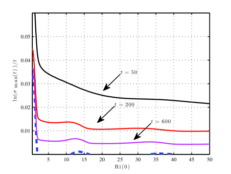
Figure 15: (Color online) Comparison of the finite time Lyapunov exponent, $\ln{\left(\sigma_{\max}(t)\right)}/t$ (solid), associated with the growth of optimal perturbations for optimizing times $t=50$, $t=200$ and $t=600$, with the modal growth rate $kc_{i}$ (dashed) for various Richardson numbers. The first three unstable Holmboe branches are shown. The H1 branch is for $\text{Ri}(0)<1.42$. The H2 branch is for $10.46\leq\text{Ri}(0)\leq 16.26$; and H3 is for $31.04\leq\text{Ri}(0)\leq 39.63$. The optimal growth rate is almost constant for large Richardson numbers and is continuous across the islands of instability. Parameters are: $k=1$ and $R=3$.

We calculate the optimal growth for two indicative optimizing times $t=100$ and $t=600$ and plot the finite time Lyapunov exponent $\ln{\left(\sigma_{\max}(t)\right)}/t$ associated with the optimal perturbations as a function of wavenumber $k$ and stratification $J$. As $t\rightarrow\infty$ the exponent tends to the modal growth rate $\ln{\left(\sigma_{\max}(t)\right)}/t\rightarrow kc_{i}$. We saw that the modal growth rate (cf. FIG. 4) is non zero only in narrow bands of parameter space. In contrast, the growth rate associated with the optimal perturbations covers all parameter space. For example, for optimizing time $t=100$ the finite Lyapunov exponent, shown in FIG. 13, is almost constant for large Richardson numbers and the equivalent growth rates for large Richardson numbers are at least an order of magnitude larger than the modal growth rates for all values of the parameters. Furthermore the growth rates do not reveal the underlying bands of exponential instability. The optimal growth is robust even for optimizing time $t=600$. Contours of the finite Lyapunov exponents for this optimizing time (FIG. 14) show that the optimal growth rates continue to be at least an order of magnitude larger than the modal growth rate for all parameter values. Moreover the optimal growth rates are almost constant as a function of Richardson number for large Richardson numbers. This can be seen in FIG. 15 where we compare the optimal growth rate for optimizing times $t=50,\ 200,\ 600$ with the modal growth rate as a function of the stratification at the center $\text{Ri}(0)$ for $k=1$. While the modal growth rate is only substantial for the H1 branch of instability the optimal growth rates produce sustainable growth at all stratifications and is reduced by a factor of less than 2 when the center Richardson number increases tenfold from 5 to 50.

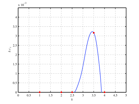
Figure 16: (Color online) Modal growth rate $kc_{i}$ as a function of wavenumber $k$ for center Richardson number $\text{Ri}(0)=5$. The instability for $2.6<k<3.9$ corresponds to the H1 branch. The dots indicate the growth rate at $k=1,\ 2,\ 2.5,\ 4$ and at $k=3.5$ when the maximum growth rate occurs.

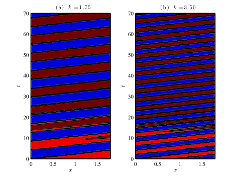
Figure 17: (Color online) Contours of the logarithm of the positive real part of the perturbation $\Re(\hat{\psi}(z,t)e^{ikx})$ at $z=0.7$ in the $(x,t)$ plane for an initial perturbation in the form of the adjoint in the energy norm of the most unstable Holmboe mode at $k=3.5$ for $R=3$ and $\text{Ri}(0)=5$. Panel (a): evolution under the dynamics with $k=1.75$ when the flow is stable. Panel (b): evolution under the dynamics with $k=3.5$ when the flow is unstable and this adjoint excites optimally the prograde Holmboe mode. The same propagation characteristics emerge at other wavenumbers for which the flow is stable. These Hovmöller diagrams indicate that when the flow is stable a quasi-mode emerges propagating with phase speed close to that of the Holmboe mode.

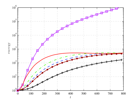
Figure 18: (Color online) Energy evolution of a unit energy initial condition with the structure of the adjoint in the energy norm of the unstable H1 mode at $k=3.5$, $R=3$ and $\text{Ri}(0)=5$ with the dynamical operator (a) for the unstable $k=3.5$ (solid-squares), (b) for $k=1.0$ (solid crosses), $k=1.75$ (solid-dots), $k=2.0$ (dashed), $k=2.5$ (dash-dot) and $k=4.0$ (solid) for which the flow is stable. When the flow is stable large amplitude propagating quasi-modes emerge as shown in FIG. 17.

The structure of the optimal perturbations for the larger optimizing times is very close to the structure of the adjoint of the modes, even for wavenumbers for which there is no Holmboe instability. This reveals that excitation of these flows at high Richardson numbers will lead to the emergence of propagating perturbations which are close in structure to Holmboe waves. To be specific, consider central stratification $\text{Ri}(0)=5$ and excitation of the shear layer with various wavenumbers $k$. In FIG. 16 we plot the growth rate as a function of $k$. There is a band of instability producing H1 waves with phase speeds close to $c_{r}\approx\pm 0.5$ and when the flow is excited at these wavenumbers pairs of propagating waves emerge. This can be seen in the Hovmöller diagram FIG. 17(b) in which contours of the logarithm of the positive real part of $\Re(\hat{\psi}(z,t)e^{ikx})$ for $k=3.5$ and fixed $z=0.7$ are plotted in the $(x,t)$ plane for an initial condition in the form of the adjoint of the unstable H1 mode. The characteristics of the prograde propagating Holmboe wave emerge from the start. In FIG. 17(a) we plot the corresponding Hovmöller diagram when the same adjoint is introduced as initial condition and evolved this time with the dynamics for $k=1.75$. Although at $k=1.75$ there is no instability, a propagating structure emerges with the characteristics of the unstable Holmboe wave. The same propagating structure also emerges at other wavenumbers $k$. Therefore the Holmboe wave is a robust dynamic entity that forms a quasi-mode at wavenumbers which do not support an unstable Holmboe wave. This quasi-mode is the manifestation of the near resonant edge wave structures that lead to the Holmboe instability at resonanceHolmboe (1962); Baines and Mitsudera (1994); Caulfield (1994); Haigh and Lawrence (1999); Harnik et al. (2008); Carpenter et al. (2010). Similar quasi-mode behavior is seen in the evolution of the edge waves in the Holmboe profile (cf. Appendix A) for wavenumbers $k$ for which there is no instability. When $k$ is close to the wavenumber for which there is instability the edge wave complex periodically amplifies while propagating at a phase speed close to the phase speed of the unstable Holmboe modes. What is surprising here is that these propagating quasi-modes can be excited at such high amplitude and that their growth is so persistent. This is shown in FIG. 18 where the adjoint of the Homboe instability for $k=3.5$ excites at high amplitude quasi-modes for the wavenumbers $k=1,\ 2,\ 2.5,\ 4$ for which the flow is stable. The same highly amplified quasi-mode would emerge if we initialize the flow with a large time optimal.

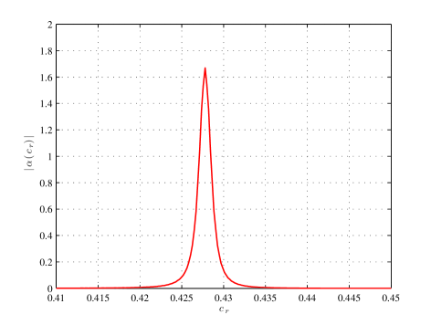
Figure 19: (Color online) Amplitude, $|\alpha(c_{r})|$, of the absolute value of the expansion coefficients of the quasi-mode at $k=1.75$ as a function of the phase speed of the modes of the perturbation operator at $k=1.75$. All the modes of the perturbation operator are stable. The quasi-mode is excited by a unit energy initial condition with the structure of the adjoint of the unstable mode for $k=3.5$. Notice the sharp peak at $c_{r}\approx 0.4278$ which indicates the formation of long-lived quasi-modes that propagate with this phase speed (see FIG. 17(a)). For $R=3$ and $\text{Ri}(0)=5$.

The structure of the quasi-mode can not be ascribed to the structure of any single mode of the operator. The quasi-mode is the superposition of a multitude of continuum spectrum modes. The quasi-mode can propagate as a coherent entity at a single phase speed because the distribution of the amplitude of the coefficients of the modal expansion is sharply peaked at the phase speed of the propagation of the quasi-mode (the amplitude of the coefficients is time invariant because all modes have zero growth). For example, the distribution of the amplitude of coefficients of the modal expansion of the quasi-mode for $k=1.75$ in FIG. 19, is concentrated at the phase speed $c_{r}\approx\pm 0.4278$ which is exactly the phase speed that emerges in FIG. 17(a).

The quasi-mode can be identified from the frequency response of the perturbation dynamics to harmonic forcing. Because the operators are either neutral or unstable in order to obtain steady harmonic response we introduce a linear damping in the dynamics, that does not affect the eigenstructures, and consider the frequency response of the stable operators $\tilde{\mathbb{A}}_{\mathbb{M}}=\mathbb{A}_{\mathbb{M}}-0.02\,\mathbb{1}$, where $\mathbb{1}$ is the identity. The steady state harmonic response, $\tilde{\psi}(z,\omega)$, where $\hat{\psi}(z,t)=\tilde{\psi}(z,\omega)e^{i\omega t}$, to harmonic forcing $\mathbb{F}e^{i\omega t}$ is then given by

$$\tilde{\psi}(z,\omega)=\mathbb{R}_{k}(\omega)\mathbb{F}~{},$$ (27)

where $\mathbb{R}_{k}(\omega)$ is the resolvent given by

$$\mathbb{R}_{k}(\omega)=(i\omega\mathbb{1}-\tilde{\mathbb{A}}_{\mathbb{M}})^{-1}~{}.$$ (28)

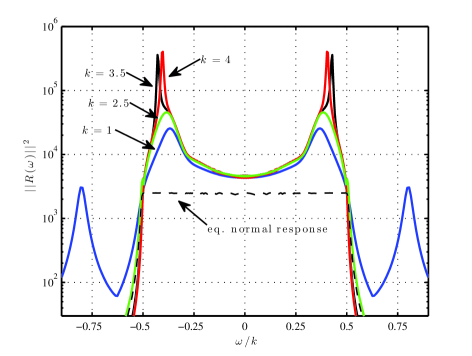
Figure 20: (Color online) The maximum energy response, $||\mathbb{R}(\omega)||^{2}$, to harmonic forcing as a function of $\omega/k$ for perturbations with $k=1$, $k=2.5$, $k=3.5$ and $k=4.0$. The dynamics have been rendered stable by addition of Rayleigh friction. The response is maximized at the phase speed of the quas-mode. Also shown is the resonant frequency response that would obtain if the operators were normal (dashed). The amplified response in energy is a measure of the non-normality of the operator. For stratification $\text{Ri}(0)=5$ and $R=3$.

The maximum possible response to harmonic forcing is then given by the square of the 2-norm of the resolvent, $||\mathbb{R}_{k}(\omega)||^{2}$, which is equal to the square of its largest singular value. This determines the maximum energy that can be achieved at frequency $\omega$ by unit energy harmonic excitation. The frequency response shown in FIG. 20 demonstrates the concentration of the response at the phase speeds of the emergent quasi-modes which is very close to the phase speed of the Holmboe waves at $k=3.5$. It demonstrates also the importance of the non-normal interactions in the excitation at high amplitude of the quasi-modes. In the same plot we plot the equivalent normal frequency response

$$\max_{j}\frac{1}{|i\omega-ikc_{j}|^{2}}~{},$$ (29)

where $ikc_{j}$ is the $j$-th eigenvalue of $\mathbb{A}_{\mathbb{M}}$ that would have resulted if the eigenvectors were orthogonal. The difference between the responses reflects the excess energy that is maintained by the system against friction because of the non-orthogonality of the eigenmodesFarrell and Ioannou (1994); Ioannou (1995).

VI Conclusions

Highly stratified shear layers are susceptible to Holmboe instabilities which can lead to mixing. We have demonstrated in this work that especially at large Richardson numbers the adjoint of the weakly unstable modes can excite, through potent transfer of energy from the mean flow, the unstable modes at high amplitude. Further we found, that even in regions of parameter space where the flow is neutral, optimal perturbations can grow strongly and excite at large amplitude long-lived propagating quasi-modes. We have demonstrated that the modal growth substantially underestimates the growth potential of perturbations in such highly stratified shear layers.

Appendix A Non-modal growth produced by the edge waves in the idealized Holmboe background state

We consider perturbations in Holmboe’sHolmboe (1962) idealized piecewise linear velocity profile $U_{0}(z)=z$ for $|z|\leq 1/2$ and $U_{0}(z)=z/(2|z|)$ for $|z|>1/2$ and mean density $\rho_{0}(z)=-z/|z|$ in an infinite domain. This profile has two vorticity discontinuities at $z=\pm 1/2$ and a density discontinuity at $z=0$; each vorticity discontinuity supports an edge wave and the density discontinuity supports a pair of edge waves one prograde and the other retrograde Holmboe (1962); Baines and Mitsudera (1994); Harnik et al. (2008); Rabinovich et al. (2011). Consider perturbations with streamfunction $\hat{\psi}(z,t)e^{ikx}$. A time dependent solution to the perturbation equations can be obtainedHolmboe (1962); Baines and Mitsudera (1994) by introducing solutions of the form,

$$\hat{\psi}_{1}(z,t) =A_{1}(t)e^{-k(z-1/2)},\quad{\rm for}~{}~{}z>1/2$$ (30a)

$$\hat{\psi}_{2}(z,t) =A_{2}(t)e^{-kz}+B_{2}(t)e^{kz},\quad{\rm for}~{}~{}0<z<1/2$$ (30b)

$$\hat{\psi}_{3}(z,t) =A_{3}(t)e^{-kz}+B_{3}(t)e^{kz},\quad{\rm for}~{}~{}-1/2<z<0$$ (30c)

$$\hat{\psi}_{4}(z,t) =B_{4}(t)e^{k(z+1/2)}~{},\quad{\rm for}~{}~{}0<z<1/2$$ (30d)

which reduce them, by imposing the usual continuity conditions at the discontinuity interfaces, to a set of ordinary differential equations for the evolution of the amplitudes $A$ and $B$. We choose as a state variable $\mathbf{u}(t)=\left[A_{1}(t),C_{2}(t),B_{4}(t),\eta_{0}(t)\right]^{\text{T}}$, where $\eta_{0}(t)\equiv\hat{\eta}(z=0,t)$ is the displacement at $z=0$ and $C_{2}(t)\equiv\left(A_{2}(t)+B_{2}(t)\right)e^{k/2}$. The perturbation equations are thus reduced to:

$$\frac{\text{d}\mathbf{u}}{\text{d}t}=\mathbb{A}\,\mathbf{u}~{}~{},$$ (31)

with $\mathbb{A}=\mathbb{K}^{-1}\mathbb{L}$ with the matrices $\mathbb{K}$ and $\mathbb{L}$ given by:

$$\mathbb{K} =\left[\begin{array}[]{cccc}-e^{k}&1&0&0\\ 2&-2\left(1+e^{-k}\right)&2&0\\ 0&1&-e^{k}&0\\ 0&0&0&1\end{array}\right]~{}~{},$$ (32e)

$$\mathbb{L} =i\left[\begin{array}[]{cccc}\left(1+e^{k}(k-1)\right)/2&-k/2&0&0\\ 0&0&0&J\left(e^{k/2}-e^{-k/2}\right)\\ 0&k/2&-\left(1+e^{k}(k-1)\right)/2&0\\ 0&-ke^{-k/2}&0&0\end{array}\right]~{}.$$ (32j)

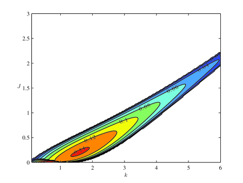
Figure 21: (Color online) Contours of modal growth rate $kc_{i}$ as a function of wavenumber, $k$, and stratification parameter, $J$, of perturbations in Holmboe’s idealized piecewise constant background state. At larger values of $k$ and $J$ there is a band of instability associated with the Holmboe instability.

These equations determine the time evolution of the perturbation structure as determined by the interaction of the four edge waves. It determines fully the modal stability properties of the background state and the non-normal dynamics that derive from the interaction of the edge waves. In this formulation we have neglected the continuum spectrum. A contour plot of the resulting growth rate is shown in FIG. 21 as a function of wavenumber, $k$, and stratification parameters, $J$. The KH branch of instability is at low $k$ and $J$ and the narrowing band of the Holmboe mode of instability at larger $k$ and $J$.

In order to study the non-normal dynamics associated with the edge waves we must introduce the corresponding to (15) energy metric. The potential energy, since $\rho_{0}^{\prime}=-\delta(z)$, is $P=\frac{1}{4}J\,\left|\eta_{0}\right|^{2}$. The kinetic energy can be written as:

$$\begin{split}T=&\frac{1}{4}\times\left(\left.-\hat{\psi_{1}}^{*}\,\text{D}\hat{\psi_{1}}\right|_{z=1/2}+\left.\hat{\psi_{2}}^{*}\,\text{D}\hat{\psi_{2}}\right|_{z=1/2}-\left.\hat{\psi_{2}}^{*}\,\text{D}\hat{\psi_{2}}\right|_{z=0}\right)\\ &+\frac{1}{4}\times\left(\left.\hat{\psi_{3}}^{*}\,\text{D}\hat{\psi_{3}}\right|_{z=0}-\left.\hat{\psi_{3}}^{*}\,\text{D}\hat{\psi_{3}}\right|_{z=-1/2}+\left.\hat{\psi_{4}}^{*}\,\text{D}\hat{\psi_{4}}\right|_{z=-1/2}\right)~{}.\end{split}$$ (33)

We thus derive that the perturbation energy of the state $\mathbf{u}(t)$ is given by

$$E=\mathbf{u}^{\dagger}\mathbb{M}\mathbf{u}$$ (34)

with the metric, $\mathbb{M}$, given by

$$\mathbb{M}=\frac{1}{4}\left[\begin{array}[]{cc}\mathbb{M}_{\textrm{T}}&0\\ 0&J\end{array}\right]$$ (35)

where $\mathbb{M}_{\textrm{T}}$ is:

$$\mathbb{M}_{\textrm{T}}=\frac{2k}{\left(e^{k}-1\right)}\left[\begin{array}[]{ccc}e^{k}&-1&0\\ -1&1+e^{-k}&-1\\ 0&-1&e^{k}\end{array}\right]$$ (36)

The non-modal growth associated by the dynamics of the edge waves is obtained by calculating the optimal energy growth that can be achieved at time $t$ which is given by:

$$E_{\textrm{opt}}(t)=||\exp(\mathbb{A}_{\textrm{M}}t)||^{2}$$ (37)

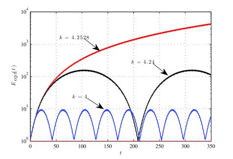
Figure 22: (Color online) Optimal energy growth that can be produced by the edge waves as a function of time for stratification parameter $J=1.5$ for $k=4.2528,~{}4.24,~{}4$. All $k\leq 4.2528$ are modally stable ($kc_{i}=0$) and $k=4.2528$ is located at the stability boundary. The non-modal growth produced by the edge waves is substantial as the stability boundary is approached.

where $\mathbb{A}_{\textrm{M}}=\mathbb{M}^{1/2}\mathbb{A}\mathbb{M}^{-1/2}$. It can be shown that the edge waves can lead to substantial growth for parameter values for which there is no instability but are close to the stability boundary. For example consider the large value of stratification $J=1.5$. The flow supports unstable waves only for $4.2528<k<5.142$ and the maximum growth rate is $0.064$. The optimal energy growth produced by the edge waves for $k=4.2528,~{}4.24,~{}4$ is shown in FIG. 22 to be substantial as the stability boundary is approached.

References

- (1)
- Miles (1961) J. W. Miles, J. Fluid Mech. 10, 496 (1961).
- Howard (1961) L. N. Howard, J. Fluid Mech. 10, 509 (1961).
- Drazin and Reid (1981) P. G. Drazin and W. H. Reid, Hydrodynamic Stability (Cambridge University Press, Cambridge, 1981).
- Holmboe (1962) J. Holmboe, Geophys. Publ. 24, 67 (1962).
- Thorpe (1971) S. A. Thorpe, J. Fluid Mech. 46, 299 (1971).
- Browand and Winant (1973) F. K. Browand and C. Winant, Boundary Layer Meteorol. 5, 67 (1973).
- Pouliquen et al. (1994) O. Pouliquen, J.-M. Chomaz, and P. Huere, J. Fluid Mech. 266, 277 (1994).
- Caulfield et al. (1995) C. P. Caulfield, W. R. Peltier, S. Yoshida, and M. Ohtani, Phys. Fluids 7, 3028 (1995).
- Zhu and Lawrence (2001) D. Z. Zhu and G. A. Lawrence, J. Fluid Mech. 429 (2001).
- Hogg and Ivey (2003) A. Hogg and G. Ivey, J. Fluid Mech. 477, 339 (2003).
- Tedford et al. (2009) E. W. Tedford, R. Pieters, and G. A. Lawrence, J. Fluid Mech. 636, 137 (2009).
- Smyth et al. (1988) W. D. Smyth, G. P. Klaassen, and W. R. Peltier, Geophys. Astrophys. Fluid Dyn. 43, 181 (1988).
- Sutherland et al. (1994) B. R. Sutherland, C. P. Caulfield, and W. R. Peltier, J. Atmos. Sci. 51, 3261 (1994).
- Smyth (2006) W. D. Smyth, Phys. Fluids 18, 064104 (2006).
- Smyth and Peltier (2006) W. D. Smyth and W. R. Peltier, J. Fluid Mech. 228, 387 (2006).
- Smyth et al. (2007) W. D. Smyth, J. R. Carpenter, and G. A. Lawrence, J. Atmos. Sci. 37, 1566 (2007).
- Carpenter et al. (2007) J. R. Carpenter, G. A. Lawrence, and W. D. Smyth, J. Fluid Mech. 582, 103 (2007).
- Alexakis (2009) A. Alexakis, Phys. Fluids 21, 054108 (2009).
- Tedford (2009) E. D. Tedford, Ph.D. thesis, The University of British Columbia (Vancouver) (2009).
- Smyth and Winters (2003) W. D. Smyth and K. B. Winters, J. Phys. Oceanogr. 33, 694 (2003).
- Alexakis (2005) A. Alexakis, Phys. Fluids 17, 084103 (2005).
- Alexakis (2007) A. Alexakis, Phys. Fluids 19, 054105 (2007).
- Rayleigh (1880) L. Rayleigh, Proc. London Math. Soc. 11, 57 (1880).
- Baines and Mitsudera (1994) P. Baines and H. Mitsudera, J. Fluid Mech. 276 (1994).
- Caulfield (1994) C. P. Caulfield, J. Fluid Mech. 258, 255 (1994).
- Haigh and Lawrence (1999) S. P. Haigh and G. A. Lawrence, Phys. Fluids 11, 1459 (1999).
- Harnik et al. (2008) N. Harnik, E. Heifetz, O. M. Umurhan, and F. Lott, J. Atmos. Sci. 65, 2615 (2008).
- Rabinovich et al. (2011) A. Rabinovich, O. M. Umurhan, N. Harnik, F. Lott, and E. Heifetz, J. Fluid Mech. 670, 301 (2011).
- Carpenter et al. (2010) J. R. Carpenter, N. J. Balmforth, and G. A. Lawrence, Phys. Fluids 22, 054104 (2010).
- Bretherton (1966) F. P. Bretherton, Q. J. R. Meteorol. Soc. 92, 335 (1966).
- Sakai (1989) S. Sakai, J. Fluid Mech. 202, 149 (1989).
- Heifetz and Methven (2005) E. Heifetz and J. Methven, Phys. Fluids 17, 064107 (2005).
- Bakas and Ioannou (2009) N. A. Bakas and P. J. Ioannou, Phys. Fluids 21, 024102 (2009).
- Goldreich et al. (1986) P. Goldreich, J. Goodman, and R. Narayan, Mon. Not. R. Astron. Soc. 221, 339 (1986).
- Narayan et al. (1987) R. Narayan, P. Goldreich, and J. Goodman, Mon. Not. R. Astron. Soc. 228, 1 (1987).
- Umurhan (2010) O. M. Umurhan, A&A 521 (2010).
- Farrell and Ioannou (1996) B. F. Farrell and P. J. Ioannou, J. Atmos. Sci. 53, 2025 (1996).
- Schmid and Henningson (2001) P. J. Schmid and D. S. Henningson, Stability and Transition in Shear Flows (Springer, New York, 2001).
- Kelvin (1887) L. Kelvin, Phil. Mag. (5) 24, 188 (1887).
- Orr (1907) W. M. Orr, Proc. Roy. Irish Acad. 27, 9 (1907).
- Phillips (1966) O. M. Phillips, The Dynamics of the Upper Ocean (Cambridge University Press, Cambridge, 1966), chap. 5, pp. 178–184.
- Hartmann (1975) R. J. Hartmann, J. Fluid Mech. 71, 89 (1975).
- Farrell and Ioannou (1993a) B. F. Farrell and P. J. Ioannou, J. Atmos. Sci. 50, 2201 (1993a).
- Farrell and Ioannou (1993b) B. F. Farrell and P. J. Ioannou, Physics of Fluids 5, 2298 (1993b).
- Heifetz et al. (1999) E. Heifetz, C. H. Bishop, and P. Alpert, Q. J. R. Meteorol. Soc. 125, 2835 (1999).
- Lott (1997) F. Lott, Q. J. R. Meteorol. Soc. 123, 1603 (1997).
- Bakas and Ioannou (2007) N. A. Bakas and P. J. Ioannou, J. Atmos. Sci. 64, 1509 (2007).
- Lott et al. (2010) F. Lott, R. Plougonven, and J. Vanneste, J. Atmos. Sci. 67, 157 (2010).
- Farrell (1988a) B. F. Farrell, J. Atmos. Sci. 45, 163 (1988a).
- Farrell (1989) B. F. Farrell, J. Atmos. Sci. 46, 1193 (1989).
- Farrell and Ioannou (1993c) B. F. Farrell and P. J. Ioannou, J. Atmos. Sci. 50, 4044 (1993c).
- Farrell and Ioannou (1994) B. F. Farrell and P. J. Ioannou, Phys. Rev. Lett. 72, 1118 (1994).
- Umurhan and Heifetz (2007) O. M. Umurhan and E. Heifetz, Phys. Fluids 19, 064102 (2007).
- Hazel (1972) P. Hazel, J. Fluid Mech. 51, 39 (1972).
- Smyth and Peltier (1989) W. D. Smyth and W. R. Peltier, J. Atmos. Sci. 46, 3698 (1989).
- Smyth and Peltier (1990) W. D. Smyth and W. R. Peltier, Geophys. Astrophys. Fluid Dyn. 52, 249 (1990).
- Howard and Maslowe (1973) L. N. Howard and S. A. Maslowe, Boundary Layer Meteorol. 4, 511 (1973).
- Farrell (1988b) B. F. Farrell, Physics of Fluids 31, 2093 (1988b).
- Hill (1995) D. C. Hill, J. Fluid Mech. 292, 183 (1995).
- Marquet et al. (2009) O. Marquet, M. Lombardi, J.-M. Chomaz, D. Sipp, and D. Jacquin, J. Fluid Mech. 622, 1 (2009).
- Ioannou (1995) P. J. Ioannou, J. Atmos. Sci. 52, 1155 (1995).