Measuring the escape velocity and mass profiles of galaxy clusters beyond their virial radius

Abstract

The caustic technique uses galaxy redshifts alone to measure the escape velocity and mass profiles of galaxy clusters to clustrocentric distances well beyond the virial radius, where dynamical equilibrium does not necessarily hold. We provide a detailed description of this technique and analyse its possible systematic errors. We apply the caustic technique to clusters with mass $M_{200}\geq 10^{14}h^{-1}M_{\odot}$ extracted from a cosmological hydrodynamic simulation of a $\Lambda$CDM universe. With a few tens of redshifts per squared comoving megaparsec within the cluster, the caustic technique, on average, recovers the profile of the escape velocity from the cluster with better than $10$ percent accuracy up to $r\sim 4r_{200}$. The caustic technique also recovers the mass profile with better than 10 percent accuracy in the range $(0.6-4)\,r_{200}$, but it overestimates the mass up to 70 percent at smaller radii. This overestimate is a consequence of neglecting the radial dependence of the filling function ${\cal F}_{\beta}(r)$. The 1-$\sigma$ uncertainty on individual escape velocity profiles increases from $\sim 20$ to $\sim 50$ percent when the radius increases from $r\sim 0.1r_{200}$ to $\sim 4r_{200}$. Individual mass profiles have 1-$\sigma$ uncertainty between 40 and 80 percent within the radial range $(0.6-4)\,r_{200}$. When the correct virial mass is known, the 1-$\sigma$ uncertainty reduces to a constant 50 percent on the same radial range. We show that the amplitude of these uncertainties is completely due to the assumption of spherical symmetry, which is difficult to drop. Other potential refinements of the technique are not crucial. We conclude that, when applied to individual clusters, the caustic technique generally provides accurate escape velocity and mass profiles, although, in some cases, the deviation from the real profile can be substantial. Alternatively, we can apply the technique to synthetic clusters obtained by stacking individual clusters: in this case, the 1-$\sigma$ uncertainty on the escape velocity profile is smaller than 20 percent out to $4r_{200}$. The caustic technique thus provides reliable average profiles which extend to regions difficult or impossible to probe with other techniques.

1 Introduction

Clusters of galaxies are valuable tools to measure the cosmological parameters and test structure formation models (e.g. Voit, 2005; Diaferio et al., 2008) and the galaxy-environment connection (e.g. Skibba et al., 2009; Huertas-Company et al., 2009; Martínez et al., 2008; Domínguez et al., 2001). The evolution of the cluster abundance is a sensitive probe of the cosmological parameters because clusters populate the exponential tail of the mass function of virialised galaxy systems. Accurate mass measurements are however required to avoid the propagation of systematic errors into the estimation of the cosmological parameters. There are two families of mass estimators: those which estimate the mass profiles and those that measure the mass enclosed within a specific projected radius.

Traditionally, the estimation of the cluster mass is based on the assumptions of spherical symmetry and dynamical equilibrium: either the cluster galaxies move accordingly to the virial theorem (Zwicky, 1937), or the hot intracluster plasma which emits in the X-ray band is in hydrostatic equilibrium within the gravitational potential well of the cluster (Sarazin, 1988). More sophisticated approaches apply the Jeans equation for a steady-state system, with the velocity anisotropy parameter $\beta$ as a further unknown (The & White 1986; Merritt 1987; see Biviano 2006 for a comprehensive review of various improvements of this method).

Dynamical equilibrium is also assumed when using the mass-X-ray temperature relation to estimate the cluster mass (e.g. Pierpaoli et al. 2003; see also Borgani 2006). Both the slope and the normalization of the observed mass–temperature relation is grossly reproduced by synthetic clusters obtained with $N$-body/hydrodynamical simulations (Borgani et al., 2004). However, the presence of non–thermal pressure support (e.g., related to turbulent gas motions) and the complex thermal structure of the intra-cluster medium can significantly bias cluster mass estimates based on the application of hydrostatic equilibrium to the X–ray estimated temperature (e.g. Rasia et al., 2006; Nagai et al., 2007; Piffaretti & Valdarnini, 2008). In principle, one can improve the mass estimate by exploiting the integrated Sunyaev-Zel’dovich effect, which depends on the first power of the gas density, rather than the square of the density as in the X-ray emission, and yields a correlation with mass which is tighter than the mass-X-ray temperature relation (e.g. Motl et al., 2005; Nagai, 2006). Only recently, such results have been confirmed by observations of real clusters (Rines et al., 2010; Andersson et al., 2010). However, their confirmation over a large statistical ensemble has to await the results from ongoing large Sunyaev-Zel’dovich surveys. Alternatively, one can bypass the problematic gas physics and use the correlation between mass and optical richness, which is relatively easy to obtain from observations in the optical/near-IR bands, but returns mass with a poorer accuracy (Andreon & Hurn, 2010).

The dynamical equilibrium assumption can be dropped in the gravitational lensing techniques, because the lensing effect depends only on the amount of mass along the line of sight and not on its dynamical state (e.g. Schneider, 2006). It is relevant to emphasize that all these methods do not measure the cluster mass on the same scale: optical observations measure the mass within $\sim r_{200}$, where $r_{200}$ is the radius within which the average mass density is 200 times the critical density of the universe; X-ray estimates rarely go beyond $\sim 0.5r_{200}$, where the X-ray surface brightness becomes smaller than the X-ray telescope sensitivity; lensing measures the central mass within $\sim 0.1r_{200}$ or the outer regions at radii larger than $\sim r_{200}$ depending on whether the strong or weak regime applies. Scaling relations do not provide any information on the mass profile and give the total mass within a radius depending on the scaling relation used, but still within $\sim r_{200}$.

Diaferio & Geller (1997) (DG97, hereafter) suggested a novel method, the caustic technique, to estimate the mass from the central region out to well beyond $r_{200}$ with galaxy celestial coordinates and redshifts alone and without assuming dynamical equilibrium (Diaferio, 2009). Prompted by the $N$-body simulations of van Haarlem & van de Weygaert (1993), DG97 noticed that in hierarchical models of structure formation, the velocity field in the cluster outskirts is not perfectly radial, as expected in the spherical infall model (Regös & Geller 1989; Hiotelis 2001) but has a substantial random component. They thus suggested to exploit this fact to extract the galaxy escape velocities as a function of radius from the distribution of galaxies in redshift space. In the caustic method, the velocity anisotropy parameter $\beta$ and the mass density profile in hierarchical clustering models combine in such a way that their knowledge is largely unnecessary in estimating the mass profile. This property explains the power of the method.

This method is particularly relevant because it is an alternative to lensing to measure mass in the cluster external regions and, unlike lensing, it can be applied to clusters at any redshift, provided there are enough galaxies to sample the redshift diagram properly. We will see below that a few tens of redshifts per squared comoving megaparsec within the cluster are sufficient to apply the technique reliably. This request might have appeared demanding a decade ago, but it is perfectly feasible for the large redshift surveys currently available.

Geller, Diaferio, & Kurtz (1999) were the first to apply the caustic method: they measured the mass profile of Coma out to $10h^{-1}$ Mpc from the cluster centre and were able to demonstrate that the Navarro, Frenk, & White (1997) (NFW) profile fits well the cluster density profile out to these very large radii, thus ruling out the isothermal sphere as a viable cluster model; a few years later, the failure of the isothermal model was confirmed by the first analysis based on gravitational lensing applied to Cl 0024 (Kneib et al., 2003). The goodness of the NFW fit out to $5-10h^{-1}$ Mpc was confirmed by applying the caustic technique to a sample of nine clusters densely sampled in their outer regions, the Cluster And Infall Region Nearby Survey (CAIRNS, Rines et al. 2003), and later to a complete sample of 72 X-ray selected clusters with galaxy redshifts extracted from the Fourth Data Release of the Sloan Digital Sky Survey (Cluster Infall Regions in the Sloan Digital Sky Survey: CIRS, Rines & Diaferio 2006) and from the Fifth Data Release (Rines & Diaferio, 2010). CIRS is currently the largest sample of clusters whose mass profiles have been measured out to $\sim 3r_{200}$; Rines & Diaferio (2006) were thus able to obtain a statistically significant estimate of the ratio between the masses within the infall and the virial regions: they found a value of $2.2\pm 0.2$, in agreement with current models of cluster formation. These analyses have been extended to a sample of groups of galaxies (Rines & Diaferio, 2010). Rines, Diaferio, & Natarajan (2007) also used the CIRS sample to estimate the virial mass function of nearby clusters and determined cosmological parameters consistent with WMAP values (Dunkley et al., 2009).

A good fit with the NFW profile out to $\sim 2r_{200}$ was also found by Biviano & Girardi (2003) who applied the caustic technique to an ensemble cluster obtained by stacking 43 clusters from the Two Degree Galaxy Redshift Survey (2dGFRS, Colless et al. 2001). Here, unlike the previous analyses, the caustic method was not applied to individual clusters because the number of galaxies per cluster was relatively small. Recently, Lemze et al. (2009) have applied both the caustic technique and the Jeans analysis to $\sim 500$ cluster members of A1689. The estimated virial mass from both methods agrees with previous lensing and X-ray analyses.

The caustic method does not rely on the dynamical state of the cluster and of its external regions: there are therefore estimates of the mass of unrelaxed systems, namely the Shapley supercluster (Reisenegger et al., 2000; Proust et al., 2006), the Fornax poor cluster, which shows two distinct dynamical components (Drinkwater, Gregg, & Colless, 2001), the A2199 complex (Rines et al., 2002), and two clusters, A168 and A1367, which are undergoing major mergers (Rines et al., 2003). More recently, Diaferio et al. (2005b) analysed Cl 0024, a cluster that is likely to have suffered a recent merging event (Czoske et al., 2002), and showed that the caustic mass and the lensing mass agree with each other, but disagree with the X-ray mass, which is the only estimate relying on dynamical equilibrium.

The method was shown to return reliable mass profiles when applied to synthetic clusters extracted from $N$-body simulations. However, these analyses of the performance of the method either were done when the operative procedure of the technique was not yet completely developed (DG97) or the results of a fully detailed analysis of the systematic errors was not provided (Diaferio, 1999) (D99, hereafter). The dense redshift surveys currently available, especially around clusters, provide ideal data sets where the caustic technique can now be applied. With this perspective, it is therefore timely to reconsider the possible systematic errors and biases of this technique, in view of a robust application to the new data sets.

The purpose of this paper is to provide both a transparent description of the technique, with some improvements to what is described in D99, and a thorough statistical analysis. The caustic technique represents a powerful method to infer cluster mass profiles and complements other methods based on X-ray, Sunyaev-Zeldovich and lensing observations which probe different scales of the clusters.

In Section 2 we describe the basic idea of the caustic technique. Section 3 describes the simulated cluster sample used, and Section 4 describes the implementation of the technique. In Sections 5.2 and 5.3 we estimate the accuracy of the escape velocity and mass profiles of galaxy clusters estimated with the caustic technique. In Section 6 we investigate the systematics due to the choice of the parameters. We summarize our main results and draw our conclusions in Section 7.

2 Basics

In this section, we briefly review the simple physical idea behind the caustic technique. More details are given in DG97 and D99.

In hierarchical clustering models of structure formation, clusters form by the aggregation of smaller systems falling onto the cluster from the surrounding region. The accretion does not take place purely radially (e.g. White et al., 2010), therefore galaxies or dark matter particles within the falling clumps have velocities with a substantial non-radial component. Specifically, the r.m.s. $\langle v^{2}\rangle$ of these velocities is due to the gravitational potential of the cluster and the groups where the galaxy resides, and to the tidal fields of the surrounding region. When viewed in the redshift diagram, viz. the plane of the line-of-sight (l.o.s.) velocity w.r.t. the cluster centre and the clustrocentric radius $r$, galaxies populate a region with a characteristic trumpet shape with decreasing amplitude ${\cal A}$ with increasing $r$. This amplitude is related to $\langle v^{2}\rangle$. The breakthrough of DG97 was to identify this amplitude with the escape velocity from the cluster region corrected for a function depending on the velocity anisotropy parameter $\beta$.

Assuming a spherically symmetric system, the escape velocity $v_{\rm esc}^{2}(r)=-2\phi(r)$, where $\phi(r)$ is the gravitational potential originated by the cluster, is a non-increasing function of $r$, because gravity is always attractive and ${\rm d}\phi/{\rm d}r>0$. At any given radius $r$, we expect that observing a galaxy with a velocity larger than the escape velocity is unlikely. Thus, we identify the escape velocity with the maximum velocity that can be observed. It follows that the amplitude ${\cal A}$ at the projected radius $r_{\perp}$ measures the average component along the l.o.s. of the escape velocity at the three-dimensional radius $r=r_{\perp}$. To determine this average component of the velocity, we consider the velocity anisotropy parameter $\beta(r)=1-(\langle v^{2}_{\theta}\rangle+\langle v^{2}_{\phi}\rangle)/2\langle v^{2}_{r}\rangle$, where $v_{\theta}$, $v_{\phi}$, and $v_{r}$ are the longitudinal, azimuthal and radial components of the velocity ${\mathbf{v}}$ of a galaxy, respectively, and the brackets indicate an average over the velocities of the galaxies in the volume $\mbox{d}^{3}{\bf r}$ centred on position ${\bf r}$. If the cluster rotation is negligible, $\langle v^{2}_{\theta}\rangle=\langle v^{2}_{\phi}\rangle=\langle v^{2}_{\rm los}\rangle$, where $v_{\rm los}$ is the l.o.s. component of the velocity, and $\langle v^{2}_{r}\rangle=\langle v^{2}\rangle-2\langle v^{2}_{\rm los}\rangle$. By substituting in the definition of $\beta$, we obtain $\langle v^{2}\rangle=\langle v^{2}_{\rm los}\rangle g(\beta)$ where

$$g(\beta)={3-2\beta(r)\over 1-\beta(r)}\;.$$ (1)

By applying this relation to the escape velocity at radius $r$, $\langle v_{\rm esc}^{2}(r)\rangle=-2\phi(r)$, and assuming that ${\cal A}^{2}(r)=\langle v^{2}_{\rm esc,los}\rangle$, we obtain the fundamental relation between the gravitational potential $\phi(r)$ and the observable caustic amplitude ${\cal A}(r)$

$$-2\phi(r)={\cal A}^{2}(r)g(\beta)\equiv\phi_{\beta}(r)g(\beta)\;.$$ (2)

Note that the gravitational potential profile is related to the caustic amplitude by the function $g(\beta)$. Therefore, after the caustic amplitude estimation, $\beta$ becomes the only unknown function for the gravitational potential estimation.

The further novel suggestion of DG97 is to use this relation to infer the cluster mass to very large radii. To do so, one first notices that the mass of an infinitesimal shell can be cast in the form $G\,\mbox{d}m=-2\phi(r){\cal F}(r)\,\mbox{d}r={\cal A}^{2}(r)g(\beta){\cal F}(r)\,\mbox{d}r$ where

$${\cal F}(r)=-2\pi G{\rho(r)r^{2}\over\phi(r)}\;.$$ (3)

Therefore the mass profile is

$$GM(<r)=\int_{0}^{r}{\cal A}^{2}(r){\cal F}_{\beta}(r)\,\mbox{d}r$$ (4)

where ${\cal F}_{\beta}(r)={\cal F}(r)g(\beta)$.

Equation (4) however only relates the mass profile to the density profile of a spherical system and a profile can not be inferred without knowing the other. DG97 solve this impasse by noticing that in hierarchical clustering scenarios, ${\cal F}(r)$ is not a strong function of $r$. This is easily seen in the case of the NFW model which is an excellent description of dark matter density profiles in the hierarchical clustering scenario:

$${\cal F}_{\rm NFW}(r)={r^{2}\over 2(r+r_{s})^{2}}{1\over\ln(1+r/r_{s})}\;,$$ (5)

where $r_{s}$ is a scale factor. One expects that ${\cal F}_{\beta}(r)$ is also a slowly changing function of $r$ if $g(\beta)$ is. DG97 and D99 show that this is the case, and here we confirm their result. The final, somewhat strong, assumption is then to consider ${\cal F}_{\beta}(r)={\cal F}_{\beta}={\rm const}$ altogether and adopt the recipe

$$GM(<r)={\cal F}_{\beta}\int_{0}^{r}{\cal A}^{2}(r)\,\mbox{d}r\;.$$ (6)

It is appropriate to emphasize that equations (2) and (4) are rigorously correct, whereas equation (6) is a heuristic recipe to estimate the mass profile. Based on equation (2) the caustic technique can also estimate a combination of the gravitational potential profile and velocity anisotropy parameter $\beta$. Below, we show the accuracy of these estimates.

3 The simulated cluster sample

Before analysing the systematic errors of the caustic technique, we need to check how well the physical assumptions of the method are satisfied. We do so by using $N$-body simulations, assuming that these simulations are a faithful representation of the real universe.

Here we use the cluster sample extracted from the cosmological $N$-body/hydrodynamical simulation described in Borgani et al. (2004). They simulate a cubic volume, 192 $h^{-1}$ Mpc on a side, of a flat $\Lambda$CDM universe, with matter density $\Omega_{0}=0.3$, Hubble parameter $H_{0}=100h$ km s^-1 Mpc^-1 with $h=0.7$, power spectrum normalization $\sigma_{8}=0.8$, and baryon density $\Omega_{\rm b}=0.02h^{-2}$. The density field is sampled with $480^{3}$ dark matter particles and an initially equal number of gas particles, with masses $m_{\rm DM}=4.6\times 10^{9}h^{-1}M_{\odot}$ and $m_{\rm gas}=6.9\times 10^{8}h^{-1}M_{\odot}$, respectively. The Plummer-equivalent gravitational softening is set to 7.5 $h^{-1}$ physical kpc at $z<2$, while being fixed in comoving units at higher redshift.

The simulation was run with GADGET-2 (Springel, Yoshida, & White, 2001), a massively parallel Tree+SPH code with fully adaptive time–stepping. Besides standard hydrodynamics, it also contains a treatment of radiative gas cooling, star formation in a multi-phase inter-stellar medium and feedback from supernovae in the form of galactic ejecta (e.g., Borgani et al., 2004; Diaferio et al., 2005a). Here we are only interested in the gravitational dynamics of the matter distribution.

The simulation volume yields a cluster sample large enough for statistical purposes. We identify clusters in the simulation box with a two-step procedure: a friends-of-friends algorithm applied to the dark matter particles alone provides a list of halos whose centres are used as input to the spherical overdensity algorithm which outputs the final list of clusters (Borgani et al., 2004). Centred on the most bound particle of each cluster, the sphere with virial overdensity 200, with respect to the critical density, defines the virial radius $r_{200}$. At redshift $z=0$ the simulation box contains 100 clusters with mass $M(<r_{200})\geq 10^{14}h^{-1}M_{\odot}$. This cluster set is our reference sample.

3.1 Cluster properties in 3D

Figure 1: Concentration parameters $c$ vs. the cluster mass $M_{200}^{\rm NFW}$ of our simulated cluster sample.

Figure 2: Profiles of the ratio between the mass profile of each cluster predicted by the NFW fit and its true mass profile: 90 (50) percent of the profiles are within the upper and lower dotted (solid) curves. The central solid curve is the median profile. For each cluster, the NFW fit is only performed to the mass distribution within $1h^{-1}$ Mpc.

Figure 3: Profiles of the ratio between the gravitational potential profile of each cluster predicted by the NFW fit and the numerical gravitational potential profile derived from the true mass distribution within $r_{\rm max}=10h^{-1}$ Mpc from the cluster centre: 90 (50) percent of the profiles are within the upper and lower dotted (solid) curves. The central solid curve is the median profile. The lower and upper dashed curves are the median profiles for $r_{\rm max}=8$ and $6h^{-1}$ Mpc, respectively.

We fit the three-dimensional (3D) real cumulative mass profile with the NFW model

$$M(<r)=M_{s}\left[\ln\left(1+{r\over r_{s}}\right)-{r/r_{s}\over 1+r/r_{s}}\right]$$ (7)

where $M_{s}=M(<r_{s})/(\ln 2-1/2)=4\pi\delta_{c}\rho_{\rm cr}r_{s}^{3}$, $\delta_{c}=(200/3)c^{3}/[\ln(1+c)-c/(1+c)]$, and $c=r_{200}^{\rm NFW}/r_{s}$. We fit the mass profile rather than the density profile to resemble the procedure adopted with real clusters (e.g. Diaferio et al., 2005b). Similarly, for the fit, we only consider the mass distribution within $r=1h^{-1}$ Mpc. Moreover, the parameters $M_{s}$ and $r_{s}$ are less correlated than $\delta_{c}$ and $r_{s}$ and adopting them in the fit provides more robust results (Mahdavi et al., 1999).

From the NFW fit we derive the parameters $r_{200}^{\rm NFW}$ and $c$. The relation between $c$ and $M_{200}^{\rm NFW}=(4\pi/3)(r_{200}^{\rm NFW})^{3}200\rho_{\rm cr}$ is shown in Figure 1. Our cluster sample provides the percentile ranges $r_{200}^{\rm NFW}=[0.77,0.86,1.17]h^{-1}{\rm Mpc}$ and $c=[2.06,4.62,6.50]$. The radius $r_{200}^{\rm NFW}$ is basically identical to the true $r_{200}$ derived from the actual mass distribution. Their ratio is $r_{200}^{\rm NFW}/r_{200}=[0.99,1.00,1.02]$. The NFW model is an excellent fit to the true mass profile (see Figure 2) within $r_{200}$. Therefore the ratio between the mass $M_{200}^{\rm NFW}$ and the actual $M_{200}$ is correspondingly close to 1: $M_{200}^{\rm NFW}/M_{200}=[0.96,1.00,1.05]$. The NFW fit is on average very good also at radii larger than $r_{200}$, although the scatter substantially increases. In the very centre, the NFW model underestimates the mass by 50 percent. This is due to the fact that the total mass includes dark matter, gas, and stars and in the simulation there is always a central galaxy which is unrealistically massive: the stellar particles, on average, contribute 50 (15) percent of the total mass within 0.02 (0.1) $r_{200}$. When the NFW fitting routine tries to accomodate the mass profile within $1h^{-1}$ Mpc, underestimating the mass profile in this very central region yields the minimum $\chi^{2}$.

The caustic amplitude is related to the gravitational potential $\phi(r)$ and we are thus interested in determining $\phi(r)$ in our simulation. For an isolated spherical system with density profile $\rho(r)$, the potential $\phi(r)$ obeying the Poisson equation can be cast in the form

$$\phi(r)=-4\pi G\left[{1\over r}\int_{0}^{r}\rho(x)x^{2}\,\mbox{d}x+\int_{r}^{\infty}\rho(x)x\,\mbox{d}x\right]\;.$$ (8)

In the real universe, the relevant quantity is the gravitational potential originating from the mass density fluctuations around the mean density $\langle\rho\rangle$. We can thus use equation (8) for non-isolated clusters by replacing $\rho(r)$ with $\rho(r)-\langle\rho\rangle\equiv\langle\rho\rangle\delta(r)$. The second integral is finite, because at sufficiently large $r$, $\delta(r)\sim 0$. In the simulation, we replace the upper limit of the second integral with $r_{\rm max}=10h^{-1}$ Mpc. Figure 3 compares $\phi_{\rm num}(r)$ computed from the actual mass distribution around each cluster in the simulation, with the gravitational potential

$$\phi_{\rm NFW}(r)=-{GM_{s}\over r}\ln\left(1+{r\over r_{s}}\right)$$ (9)

expected from an isolated cluster described by the NFW model. The NFW potential well is deeper than the numerical $\phi_{\rm num}(r)$, because it neglects the mass surrounding the cluster. This mass exerts a pull to the mass within the cluster that makes the actual $\phi_{\rm num}(r)$ to be 10–30 percent shallower. The upper limit $r_{\rm max}$ of the second integral of equation (8), adopted in the numerical estimate, plays a negligible effect when it is large enough: the median $\phi_{\rm num}(r)$ for $r_{\rm max}=8h^{-1}$ Mpc is indistinguishable from the profile computed with $r_{\rm max}=10h^{-1}$ Mpc.

Figure 4 shows the profiles of the velocity anisotropy parameter $\beta(r)$ and the other functions defined in Section 2 for our sample of 100 simulated galaxy clusters. This figure confirms the results of the $\Lambda$CDM model presented in Figure 3 of D99 (see also Figure 25 in Diaferio et al. 2001, which shows the velocity field of simulated galaxies rather than dark matter particles). Specifically, Figure 4 shows that, on average, $\beta(r)\la 0.7$ at $r\la 3r_{200}$ and consequently, on these scales, the median profile of $g(\beta)$ varies by less than 30 percent. Individual clusters may of course have wider variations.

We remind that $\beta(r)$ is derived from the velocities of all the particles in the simulations (dark matter, gas and stars). These velocities are set in the rest frame of each cluster and are augmented of the Hubble flow contribution $H_{0}{\bf r}$. This term provides an increasing contribution to the particle velocity which is not negligible at $r\ga(1-2)r_{200}$. Specifically, by assuming dynamical equilibrium and setting $v_{p}^{2}(r)\sim GM(<r)/r$, where $v_{p}(r)$ is the average peculiar velocity at $r$, we see that $v_{p}$ decreases with $r$; therefore, the total velocity ${\bf v}(r)={\bf v}_{p}(r)+H_{0}{\bf r}$ reaches a minimum value when $v_{p}(r)\sim H_{0}r$, viz. when $r\sim[GM(<r)/H_{0}^{2}]^{1/3}\sim 4.01h^{-1}$ Mpc, where we have set $M=1.49\times 10^{14}h^{-1}M_{\odot}$, the median $M_{200}$ of our cluster sample. Since the tangential component of the total velocity is unaffected by the Hubble flow, the minimum of $v_{p}(r)$, and consequently of $\langle v_{r}^{2}\rangle$, is a minimum of $\beta$. For our sample the median $r_{200}=0.86h^{-1}$ Mpc, and we have a minimum $\beta$ at $r/r_{200}=4.66$ which is in rough agreement with Figure 4.

Finally, Figure 4 shows that ${\cal F}(r)$ and ${\cal F}_{\beta}(r)$ are slowly varying functions of $r$, as expected. We discuss these profiles in Section 5.3.

Figure 4: Profiles of the functions $\beta(r)$, $g(\beta)$, ${\cal F}(r)$ and ${\cal F}_{\beta}(r)$ described in the text: 50, 68 and 90 percent of the profiles are within the upper and lower dotted, solid and dashed curves. The central solid curves are the median profiles.

3.2 The mock cluster catalogue

We compile mock redshift catalogues from our 100 simulated clusters as follows. We project each cluster along ten random lines of sight; for each line of sight, we also project the clusters along two additional lines of sight in order to have a set of three orthogonal projections for each random direction. We thus have a total of $100\times 10\times 3=3000$ mock redshift surveys. We locate the cluster centre at the celestial coordinate $(\alpha,\delta)=(6^{h},0^{\circ})$ and redshift $cz=32000$ km s^-1. We consider a field of view of $12h^{-1}$ Mpc on a side at the cluster distance. The simulation box is $192h^{-1}$ Mpc on a side, and the mock survey contains a large fraction of foreground and background large-scale structure. We only consider a random sample of 1000 dark matter particles in each mock catalogue. Only a fraction of these 1000 particles are within $3r_{200}$ of the cluster centre, specifically this number has percentile range $[96,185,408]$ in our 3000 mock catalogues. In Sect. 6.4 we investigate the effect of varying the number of particles in the mock survey.

4 The caustic Technique

The celestial coordinates and redshifts of the galaxies within the cluster field of view are the input data of the caustic technique. The technique proceeds along four major steps:

1. arrange the galaxies in a binary tree according to a hierarchical method;

2. select two thresholds to cut the tree twice, at an upper and a lower level: the largest group obtained from the upper-level threshold identifies the cluster candidate members; the lower-level threshold identifies the substructures of the cluster; the cluster candidate members determine the cluster centre, its velocity dispersion and size;

3. with the cluster centre of the candidate members, build the redshift diagram of all the galaxies in the field; with the velocity dispersion and size of the candidate members determine the threshold $\kappa$ which enters the caustic equation, locate the caustics, and identify the final cluster members;

4. the caustic amplitude determines the escape velocity and mass profiles.

We detail these steps in turn.

4.1 Binary tree

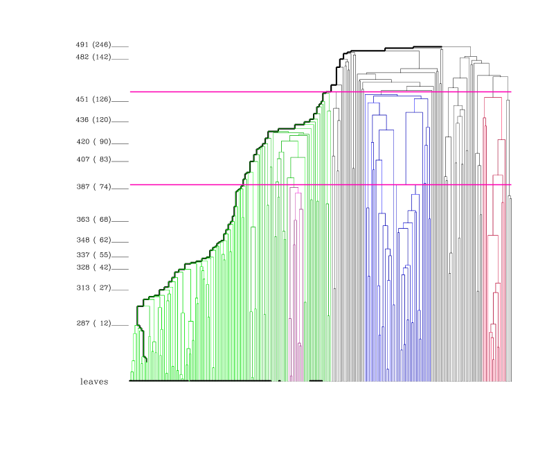
Figure 5: Dendrogram representation of the binary tree of a subsample of the particles in the field of a simulated cluster. The particles are the leaves of the tree at the bottom of the plot. The particles within $3r_{200}$ in real space are highlighted in black. The thick path highlights the main branch. The horizontal lines show the upper and lower thresholds used to cut the tree. Only as a guide, some nodes are labelled on the left-hand side, with their number of descendants in brackets.

Each galaxy is located by the vector ${\mn@boldsymbol{r}}_{i}=(\alpha_{i},\delta_{i},r_{i})$, where $\alpha_{i}$ and $\delta_{i}$ are the celestial coordinates, and $r_{i}$ is the comoving distance to the observer of a source at redshift $z_{i}$, i.e. the spatial part of the geodesic travelled by a light signal from the source to the observer. The comoving radial coordinate $r_{i}$ is determined by the relation $\int_{0}^{r_{i}}dx/\sqrt{1-\kappa x^{2}}=\int_{0}^{z_{i}}cdz/H(z)$, where $\kappa=(H_{0}/c)^{2}(\Omega_{0}+\Omega_{\Lambda}-1)$ is the space curvature and $H^{2}(z)=H_{0}^{2}[\Omega_{0}(1+z)^{3}+(1-\Omega_{0}-\Omega_{\Lambda})(1+z)^{2}+\Omega_{\Lambda}]$ is the Hubble constant at redshift $z$. In the Einstein-de Sitter universe ($\kappa=0$, $\Omega_{0}=1$)

$$r_{i}={2c\over H_{0}}\left[1-{1\over(1+z_{i})^{1/2}}\right]\;.$$ (10)

The comoving separation $r_{12}$ between two sources with comoving radial coordinates $r_{1}$ and $r_{2}$ and angular separation $\theta$ as observed from $O$ is

$$r_{12}^{2} = r_{1}^{2}+r_{2}^{2}-\kappa r_{1}^{2}r_{2}^{2}(1+\cos^{2}\theta)-2r_{1}r_{2}\cos\theta\times$$ (12)

$$\times\sqrt{1-\kappa r_{1}^{2}}\sqrt{1-\kappa r_{2}^{2}}\;.$$

This equation is a generalization of the cosine law on the two-dimensional surface of a sphere (e. g. Peebles 1993, equation 12.42).

For the construction of the binary tree, we are interested in defining an appropriate similarity based on the pairwise separation $r_{12}$. In general, the rank of the separation $r_{12}$ of a number of sources with different redshift $z_{i}$ is not preserved when we vary $\Omega_{0}$ and $\Omega_{\Lambda}$. However, a sufficient condition for having the ranks preserved is that the universe is never collapsing and $\kappa\leq 0$. This condition is satisfied when $\Omega_{0}\leq 1$ and $\Omega_{0}+\Omega_{\Lambda}\leq 1$.

Based on this argument, we can compute $r_{12}$ in the Einstein-de Sitter universe, and use the ordinary Euclidean geometry to derive the binary tree similarity. For each galaxy pair, we define the l.o.s. vector ${\mn@boldsymbol{l}}=({\mn@boldsymbol{r}}_{1}+{\mn@boldsymbol{r}}_{2})/2$ and the separation vector ${\mn@boldsymbol{r}}_{12}={\mn@boldsymbol{r}}_{1}-{\mn@boldsymbol{r}}_{2}$. We then determine the component of ${\mn@boldsymbol{r}}_{12}$ along the line of sight,

$$\pi={{\mn@boldsymbol{r}}_{12}\cdot{\mn@boldsymbol{l}}\over|{\mn@boldsymbol{l}}|}={r_{1}^{2}-r_{2}^{2}\over|{\mn@boldsymbol{r}}_{1}+{\mn@boldsymbol{r}}_{2}|}\;,$$ (13)

and the component perpendicular to the line of sight

$$r_{p}=(r_{12}^{2}-\pi^{2})^{1/2}.$$ (14)

We now consider the proper l.o.s. velocity difference $\Pi=\pi/(1+z_{l})$ and the proper projected spatial separation $R_{p}=r_{p}/(1+z_{l})$ of the galaxy pair at the intermediate redshift $z_{l}$ that satisfies the relation $r_{l}=(r_{1}+r_{2})/2$. We adopt the similarity

$$E_{ij}=-G{m_{i}m_{j}\over R_{p}}+{1\over 2}{m_{i}m_{j}\over m_{i}+m_{j}}\Pi^{2}\;.$$ (15)

This similarity reduces to the one adopted by D99 at small $z$. In equation (15), the galaxy mass is a free parameter. D99 assumes $m_{i}=m_{j}=10^{12}h^{-1}$ M_⊙, as we do here. Varying the galaxy mass changes the details of the binary tree, because one differently weights $\Pi$ and $R_{p}$. However, in the range $(10^{11},10^{13})h^{-1}$ M_⊙, the centre location and the galaxy membership remain substantially unchanged. One can of course include different galaxy masses proportional to the galaxy luminosities. This prescription turns out to be unnecessary, because it would not increase the accuracy of the determination of the mass and escape velocity profiles. In fact, we will see below (Section 6.3) that projection effects completely dominate the uncertainties of the caustic method.

For the sake of completeness, we note that, in a non-flat universe, with $\Omega_{0}<1$ and $\Omega_{0}+\Omega_{\Lambda}<1$, one can still perform the component separation with equations (13) and (14) on a flat space tangent to the observer’s location point $O$, provided one defines an appropriate bi-unique function between a geodesic distance $r_{i}$ and a vector ${\mn@boldsymbol{r}}_{i}$ on the flat space.

The binary tree is built as follows: (i) each galaxy can be thought as a group $g_{\alpha}$; (ii) to each group pair $g_{\alpha},g_{\beta}$ it is associated the binding energy $E_{\alpha\beta}={\rm min}\{E_{ij}\}$, where $E_{ij}$ is the binding energy between the galaxy $i\in g_{\alpha}$ and the galaxy $j\in g_{\beta}$; (iii) the two groups with the smallest binding energy $E_{\alpha\beta}$ are replaced with a single group $g_{\gamma}$ and the total number of groups is decreased by one; (iv) the procedure is repeated from step (ii) until we are left with only one group. Figure 5 shows the binary tree of a simulated cluster as an example.

4.2 Cutting the binary tree: The $\sigma$ plateau

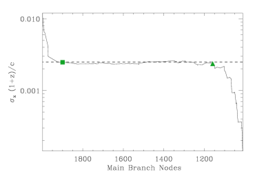
Figure 6: Velocity dispersion of the leaves of each node along the main branch of the binary tree shown in Figure 5. The filled square and triangle indicate the final thresholds (nodes $x_{1}$ and $x_{2}$) chosen by the algorithm. The dashed line shows the l.o.s. velocity dispersion of the particles within a 3D sphere of radius $3r_{200}$.

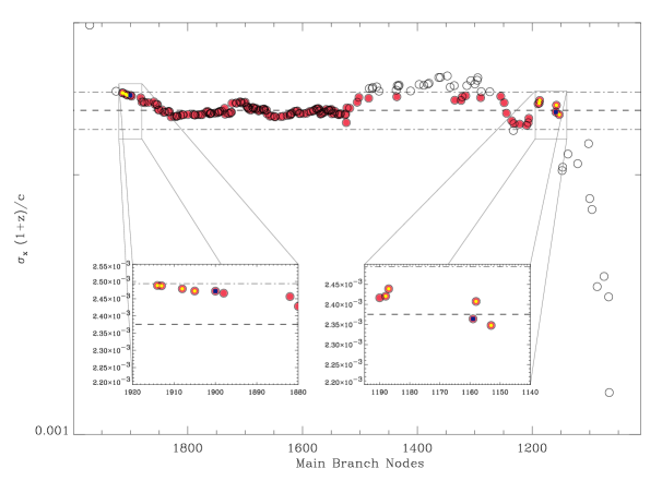
Figure 7: Line-of-sight velocity dispersion of the leaves of each node along the main branch of the binary tree shown in Figure 5. The filled red circles are the $N_{\delta}$ nodes. The dashed line indicates $\sigma_{\rm pl}$, whereas the dot-dashed lines show the range defined by equation (16): $\delta=0.05$ in this case. The ten circles with a yellow centre indicate the five nodes closest to the root and the five nodes closest to the leaves. These nodes also appear in the two insets. The two blue squares denote the two final nodes $x_{1}$ and $x_{2}$.

Gravity is a long-range force and defining a system of galaxies is somewhat arbitrary. The most widely used approach is to select a system according to a density threshold, either in redshift space, for real data, or in real space, for simulated data.

When applied to real data, the binary tree described in the previous section has the advantage of building a hierarchy of galaxy pairs with increasing, albeit projected, binding energy. The tree automatically arranges the galaxies in potentially distinct groups based on a single parameter, the galaxy mass. To get effectively distinct groups, however, we need to choose a threshold, i.e. the node from which the group members hang, where we cut the tree. This choice has been traditionally arbitrary (Materne 1978; Serna & Gerbal 1996).

D99 suggests a more objective criterion based on the following argument. We first identify the main branch of the binary tree, that is the branch that links the nodes from which, at each level of the tree, the largest number of leaves hang. The velocity dispersion $\sigma_{x}$ of the galaxies hanging from a given node $x$ shows a characteristic behaviour when walking towards the leaves along the main branch (Figure 6): initially it decreases rapidly, it then reaches a long plateau and again drops rapidly towards the end of the walk. The plateau is a clear indication of the presence of the nearly isothermal cluster: at the beginning of the walk, $\sigma_{x}$ is large because of the presence of background and foreground galaxies; at the end of the walk the tree splits into different substructures and $\sigma_{x}$ drops again.

The two nodes $x_{1}$ and $x_{2}$ that limit the $\sigma$ plateau are good candidates for the cluster/substructure identification. To locate $x_{1}$ and $x_{2}$, we proceed as follows. We consider the density distribution of the $\sigma_{x}$. The mode of this density distribution is $\sigma_{\rm pl}$. We then identify the $N_{\delta}$ nodes whose velocity dispersion $\sigma_{x}$ fulfills the inequality

$${|\sigma_{\rm pl}-\sigma_{x}|\over\sigma_{\rm pl}}\leqslant\delta\;.$$ (16)

Clearly, the number of nodes $N_{\delta}$ depends on the parameter $\delta$. We limit the parameter $\delta$ in the range $[0.03,0.1]$, but we also compute the number of nodes $N_{0.3}$ when $\delta=0.3$. We determine the number of nodes $N_{\delta}$ corresponding to increasing values of $\delta\in[0.03,0.1]$ by step of 0.01 until $N_{\delta}$ is larger than $0.8N_{0.3}$. This sets the final number of nodes $N_{\delta}$. If all the $N_{\delta}$ with $\delta\in[0.03,0.1]$ are smaller than $0.8N_{0.3}$, we choose $0.8N_{0.3}$ as the final number of nodes. The upper limit of the range of $\delta$, $\delta=0.1$, is chosen because it always provides a sufficiently large number of nodes (15 in our sample); the arbitrary threshold $0.8N_{0.3}$ is chosen because it enables to deal efficiently with particularly peaked density distributions of $\sigma_{x}$. Among the $N_{\delta}$ nodes, we locate the five nodes closest to the root and the five nodes closest to the leaves; among the former set, the final node $x_{1}$ has $\sigma_{x}$ with the smallest discrepancy from $\sigma_{\rm pl}$, and similarly for the final node $x_{2}$ among the five nodes closest to the leaves. This procedure, illustrated in Figure 7, guarantees a sufficiently large number of nodes along the $\sigma$ plateau and prevents us from locating the extrema of the $\sigma$ plateau on nodes whose $\sigma_{x}$ are too discrepant from $\sigma_{\rm pl}$.

4.3 Redshift-space diagram, caustics and final members

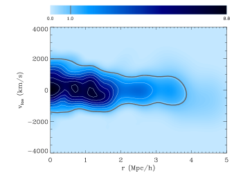
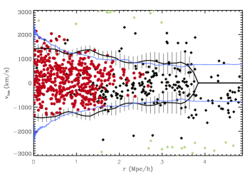
Figure 8: Left panel: the function $f_{q}(r,v)$ on the redshift diagram (colour map and contours) of the cluster shown in Figures 5-7. The thick line shows where $f_{q}(r,v)=\kappa$. Right panel: the redshift diagram of the same cluster with the upper and the lower caustics. The black and cyan lines are the estimated and true caustics respectively; the error bars are estimated with the procedure described in section 5.5. The symbols are the particles in the catalogue: the red dots are the particles within a sphere of $3r_{200}$ centred on the cluster centre, in real space; the green diamonds are the particles whose l.o.s. velocity exceeds 3.5 times the velocity dispersion $\langle v^{2}\rangle^{1/2}$ of the candidate members.

The candidate cluster members are the galaxies hanging from node $x_{1}$ and constitute the main group of the binary tree. These galaxies determine the centre and the size $R$ of the cluster. The redshift $z_{c}$ of the cluster is the median of the candidate redshifts. The celestial coordinates of the centre are the coordinates of the two-dimensional (2D) density peak of the candidates. To find the peak, we compute the 2D density distribution $f_{q}(\alpha,\delta)$ of the candidates on the sky with the kernel method described below (equation 19). In general, the smoothing parameter $h_{c}$ is automatically chosen by the adaptive kernel method. However, to save substantial computing time, here we set $h_{c}=0.15(D_{A}/320h^{-1}{\rm Mpc})$ rad, where $D_{A}(z_{c})$ is the angular diameter distance of the cluster. This choice yields accurate results. The cluster size $R$ is the mean projected separation of the candidate cluster members from the cluster centre.

We then build the redshift diagram, which is the plane $(r,v)$ of the projected distance $r$ and the l.o.s. velocity $v$ of the galaxies from the cluster centre. If $\psi$ is the angular separation between the cluster centre and a galaxy at redshift $z$, then

$$r={cD_{A}(z_{c})\over H_{0}}\sin\psi\;,$$ (17)

and

$$v=c{z-z_{c}\over 1+z_{c}}\;,$$ (18)

where we have assumed that the galaxy velocity within the cluster is much smaller than the speed of light $c$ and we have neglected the peculiar velocity of the cluster. Note that to avoid artificial depletion of the caustic amplitude at small $r$ due to the small number of galaxies in the central region, the galaxy distribution is mirrored to negative $r$. As an example, in Figure 8 we show the redshift diagram of the system shown in Figures 5-7.

It is now necessary to locate the caustics. The distribution of $N$ galaxies in the redshift diagram is described by the 2D distribution:

$$f_{q}({\bf x})={1\over N}\sum_{i=1}^{N}{1\over h_{i}^{2}}K\left({\bf x}-{\bf x}_{i}\over h_{i}\right)$$ (19)

where ${\bf x}=(r,v)$, the adaptive kernel is

$$K({\bf t})=\cases{4\pi^{-1}(1-t^{2})^{3}&$t<1$\cr 0&otherwise;\cr}$$ (20)

$h_{i}=h_{c}h_{\rm opt}\lambda_{i}$ is a local smoothing length, $\lambda_{i}=[\gamma/f_{1}({\mathbf{x}}_{i})]^{1/2}$, $f_{1}$ is equation (19) where $h_{c}=\lambda_{i}=1$ for any $i$, and $\log\gamma=\sum_{i}\log[f_{1}({\mathbf{x}}_{i})]/N$. D99 describes how the adaptive kernel method automatically determines $h_{c}$.

The optimal smoothing length

$$h_{\rm opt}={6.24\over N^{1/6}}\left(\sigma_{r}^{2}+\sigma_{v}^{2}\over 2\right)^{1/2}$$ (21)

depends on the marginal standard deviations $\sigma_{r}$ and $\sigma_{v}$ of the galaxy coordinates in the $(r,v)$ plane. These two $\sigma$’s must have the same units and we require the smoothing to mirror the uncertainty in the determination of the position and velocity of the galaxies. We therefore rescale the coordinates such that $q=\sigma_{v}/\sigma_{r}$ assumes a fixed value. We choose $q=25$. With this value, an uncertainty of 100 km s^-1 in the $v$ direction, for example, weights like an uncertainty of $0.02h^{-1}$ Mpc in the $r$ direction. The optimal smoothing length $h_{\rm opt}$ adopted by D99 is half the value we use here. However, that $h_{\rm opt}$ is derived in the context of the probability density estimate under the assumption that ${\bf x}=(r,v)$ is a normally distributed random variate with unit variance (Silverman, 1986, sects. 4.3 and 5.3). However, this assumption clearly does not apply to our context here, and we find that we obtain more accurate results with equation (21).

The caustics are now the loci of the pairs $(r,v)$ that satisfy the caustic equation

$$f_{q}(r,v)=\kappa\;,$$ (22)

where $\kappa$ is a parameter we determine below. In general, the density distribution $f_{q}(r,v)$ is not symmetric around the straight line $v=0$ in the $(r,v)$ plane, and equation (22) determines two curves $v_{\rm up}(r)$ and $v_{\rm down}(r)$, above and below this line. Because we assume spherical symmetry, we define the two caustics to be ${\cal V}_{\kappa}^{\pm}(r)=\pm{\rm min}\{|v_{\rm up}(r)|,|v_{\rm down}(r)|\}$. This choice limits the number of interlopers. The caustic amplitude is ${\cal A}_{\kappa}(r)=[{\cal V}_{\kappa}^{+}(r)-{\cal V}_{\kappa}^{-}(r)]/2$. Any realistic models of galaxy clusters has ${\rm d}\ln{\cal A}/{\rm d}\ln r\la 1/4$. A value of this derivative much larger than $1/4$ indicates that the algorithm has found an incorrect location of the caustics, which includes an excessive number of foreground and/or background galaxies. Therefore, whenever ${\rm d}\ln{\cal A}/{\rm d}\ln r>\zeta$ at a given $r$, the algorithm replaces ${\cal A}(r)$ with a new value that yields ${\rm d}\ln{\cal A}/{\rm d}\ln r=1/4$. We choose $\zeta=2$, rather than $\zeta=1/4$, to keep this constrain loose.

We choose the parameter $\kappa$, that determines the correct caustic location, as the root of the equation

$$S(\kappa)\equiv\langle v_{\rm esc}^{2}\rangle_{\kappa,R}-4\langle v^{2}\rangle=0\;,$$ (23)

where $\langle v_{\rm esc}^{2}\rangle_{\kappa,R}=\int_{0}^{R}{\cal A}_{\kappa}^{2}(r)\varphi(r){\rm d}r/\int_{0}^{R}\varphi(r){\rm d}r$ is the mean caustic amplitude within the main group size $R$, $\varphi(r)=\int f_{q}(r,v){\rm d}v$, and $\langle v^{2}\rangle^{1/2}$ is the velocity dispersion of the candidate cluster members with respect to the median redshift. When $S(\kappa)=0$, the escape velocity inferred from the caustic amplitude equals the escape velocity of a system in dynamical equilibrium with a Maxwellian velocity distribution within $R$. However, it is important to emphasize that the prescription for determining $\kappa$ works equally well for any cluster independently of its dynamical status within $R$. Therefore this prescription appears to be just a convenient recipe to locate the caustics properly and does not limit the caustic technique to systems in equilibrium within $R$.

The outcome of the process described in the preceding paragraphs is outlined in Figure 8, where ${\cal V}_{\kappa}^{\pm}(r)$ are shown together with the expected caustic amplitude $v_{\rm esc,los}(r)=\pm\sqrt{2\mid\phi(r)\mid/g(\beta)}\equiv\pm\sqrt{\phi_{\beta}(r)}$. Figure 8 shows a good agreement between the expected and estimated caustics; in Sect. 5.2, we will see that this is a general result.

4.4 Tunable parameters

The caustic technique requires two sets of parameters: a set for building the binary tree and identifying the cluster candidate members and a set for the location of the caustics in the redshift diagram. Most parameters are automatically determined by the method with the prescriptions described above. A few remaining parameters, listed in Table 1, are chosen in input. In most cases, keeping these parameters to the default value returns accurate results. In fact, in Section 6.2 we show how, in general, the improvement provided by a fine tuning of these parameters is modest.

parameter	symbol	default value
Binary tree construction and candidate members
galaxy mass	$m$	$10^{12}h^{-1}{\rm M}_{\odot}$
cluster threshold node	$x_{1}$	$-$
substructure threshold node	$x_{2}$	$-$
Caustic location
rescaling	$q$	25
smoothing length	$h_{c}$	$-$
threshold	$\kappa$	$-$
derivative limit of ${\cal A}$	$\zeta$	2
Mass profile
filling factor	${\cal F}_{\beta}$	$0.7$

Table 1: List of the tunable parameters.

5 The caustic technique at work

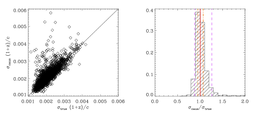
Figure 9: Comparison between the true velocity dispersion $\sigma_{\rm true}$ and the velocity dispersion of the cluster candidate members $\sigma_{\rm caus}$. The red solid line in the histogram in the right panel represents the median and the dash-dotted orange (dashed violet) lines represent the 50 (90) percent range.

We now apply the caustic method to the mock redshift catalogues described in Sect. 3.2. We describe how the technique recovers the centre and velocity dispersion of a cluster, and its escape velocity and mass profiles. Finally, we provide a simple recipe to estimate the uncertainties on these profiles.

5.1 Global properties of the cluster

In order to remove foreground and background large-scale structure from the redshift diagram, we remove all the particles with l.o.s. velocity larger than 3.5 times the velocity dispersion of the candidate members. Nevertheless, when the cluster is embedded in a particularly crowded area of the sky, it can also happen that the main branch of the tree identifies a cluster different from the target cluster. These cases can happen, for example, when the target cluster is less rich than nearby systems; they are easily solved by limiting the input particle catalogue to a small enough region centred on the target cluster. In our sample, the main branch of the binary tree identifies a cluster different from our target 326 times out of 3000, in other words only 11 percent of the times. For the sake of simplicity, we limit our sample to the 2674 clusters which are identified without further limitation of the cluster field of view.

The input centre $[\alpha,\delta,cz]=[90^{\circ},0^{\circ},32000\,{\rm km\,s}^{-1}]$, is recovered very well: the percentile ranges are $\alpha=[89.96,90.00,90.04]^{\circ}$, $\delta=[-0.040,0.000,0.036]^{\circ}$, and $cz=[31740,31998,32222]$ km s^-1.

Figure 9 shows the agreement between the estimated velocity dispersion $\sigma_{\rm caus}$ (the velocity dispersion of the galaxies hanging from the node $x_{1}$) and the true velocity dispersion $\sigma_{\rm true}$, defined as the l.o.s. velocity dispersion of the particles within a sphere of radius $3r_{200}$ in real space: in 50 (95) percent of the systems the estimated velocity dispersion is within 5 (30) percent of the real one.

5.2 The escape velocity profile

Figure 10: Profiles of the ratio between the caustic amplitude ${\cal A}(r)$ and the l.o.s. component of the true escape velocity $\langle v_{\rm esc,los}^{2}(r)\rangle=-2\phi(r)/g(\beta)\equiv\phi_{\beta}(r)$. The numerical gravitational potential profile $\phi(r)$ is derived from the true mass distribution within $r_{\rm max}=10h^{-1}$ Mpc from the cluster centre: 50, 68, and 90 percent of the profiles are within the upper and lower solid, dashed, and dotted curves, respectively. The solid squares show the median profile. The darkness of the shaded areas is proportional to the profile number density on the vertical axis.

The caustic amplitude is related to $\phi_{\beta}(r)$ (equation 2), the mean component along the line of sight of the escape velocity, which is a combination of the gravitational potential and the velocity anisotropy parameter. Figure 10 shows how well the caustic amplitude recovers $\phi_{\beta}(r)$. On average, the potential is slightly underestimated in the central region ($r\lesssim 0.2\,r_{200}$), but in the outer regions the agreement with the true escape velocity is remarkable. The slight systematic underestimate at the centre is due to the small number of particles at very small radii in the redshift diagram, that leads to an underestimate of the caustic amplitude. In the cluster outskirts, the location of the caustics is less accurate because the number of particles sampling the density distribution $f_{q}(r,v)$ is smaller. This fact increases the scatter of the profiles at large radii. We will see below that increasing the number of particles in the mock catalogues indeed reduces the scatter (Figure 20). We remind, however, that the statistical significance of the scatter decreases at increasing radii: in fact, the number of clusters contributing to the median profile decreases at large $r$, because we exclude those clusters that have a null caustic amplitude ${\cal A}(r)=0$ beyond any given radius $r$.

5.3 The mass profile

Figure 11: Profiles of the integral $\int_{0}^{r}{\cal F}_{\beta}(x){\rm d}x/r$ described in the text; 90, 68, and 50 percent of the profiles are within the upper and lower dashed, solid and dotted curves. The central solid curve is the median profile.

DG97 show that the caustic amplitude can be related to the cumulative mass profile of the cluster by the relation (4):

$$GM(<r)=\int_{0}^{r}{\cal F}_{\beta}(r){\cal A}^{2}(r)dr\;.$$

The bottom right panel of Figure 4 shows the function ${\cal F}_{\beta}(r)$ in our simulations. At radii in the range $\sim(0.5-4)r_{200}$, the average ${\cal F}_{\beta}(r)$ has a mild variation, between 0.5 and 0.8. This result led DG97 and D99 to assume ${\cal F}_{\beta}(r)={\rm const}$ tout court and assume that the mass profiles of real clusters can be estimated with the expression (6):

$$GM(<r)={\cal F}_{\beta}\int_{0}^{r}{\cal A}^{2}(r)dr\;.$$

We can choose the correct value of the factor ${\cal F}_{\beta}$ by considering the contribution of the filling function ${\cal F}_{\beta}(r)$ in the integral of equation (4). Figure 11 shows $\langle{\cal F}_{\beta}(r)\rangle=\int_{0}^{r}{\cal F}_{\beta}(x){\rm d}x/r$, where ${\cal F}_{\beta}(x)$ is the profile of each individual cluster. At radii larger than $\sim 0.5r_{200}$, $\langle{\cal F}_{\beta}(r)\rangle$ is basically constant and supports the validity of equation (6).

We see that the most appropriate value is ${\cal F}_{\beta}=0.7$. This choice disagrees with the value ${\cal F}_{\beta}=0.5$ adopted by DG97 and D99. In this early work, the algorithm for the determination of the $\sigma$ plateau was less accurate than our algorithm here and systematically provided slightly larger caustic amplitudes. This overestimate was compensated by a smaller ${\cal F}_{\beta}$, that, on turn, returned the correct mass profile, on average. Here, our improved algorithm appears to be more appropriate because it returns the correct $\phi_{\beta}(r)$ profile (Figure 10) and, in order to estimate the correct mass profile, requires a value of ${\cal F}_{\beta}$ in agreement with what can be expected by inspecting Figure 11.

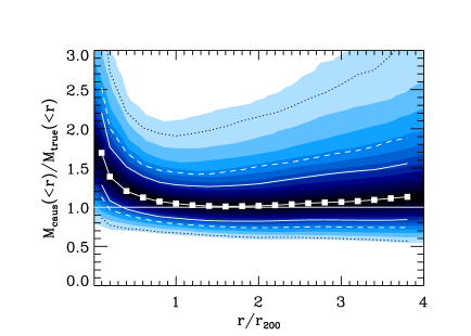
Figure 12: Profiles of the ratio between the caustic and the true mass profile, adopting equation (6) and ${\cal F}_{\beta}=0.7$. The lines and shaded areas are as in Figure 10.

Figure 12 shows that, on average, the mass profile is estimated at better than 10 percent at radii larger than $\sim 0.6r_{200}$. Clearly, at smaller radii, the assumption ${\cal F}_{\beta}(r)={\rm const}$ breaks down and the mass is severely overestimated.

As already suggested by DG97, if we assume that the cluster is in virial equilibrium in the central region, we can use the virial theorem to estimate the mass there and limit the use of the caustic method to the cluster outskirts alone, where the equilibrium assumption does not hold. Here we use the virial theorem and the median and average mass estimators from Heisler et al. (1985) to estimate the mass within $\alpha R$, where $R$ is the mean clustrocentric separation of the candidate cluster members from the binary tree (see Section 4.3) and $\alpha$ is a free parameter. In our sample, the percentile range is $R=[0.50,1.23,1.68]h^{-1}$ Mpc. We compute the ratio between the estimated mass and the true mass for different values of $\alpha$. We find that the best estimates are obtained when $\alpha=0.7$. In this case, the ratio between the estimated and true masses is, on average, $1.03$ for the virial theorem, 1.30 and 1.49 for the median and average mass estimators, respectively. Different values of $\alpha$ yield worse mass estimates. This result indicates that the radius $0.7R$ generally contains the cluster region in approximate virial equilibrium.

When we estimate the mass with the virial theorem within $0.7R$ and use equation (6) with $0.7R$ as the lower limit of the integral, we still obtain a very good estimate of the real mass (Figure 13).

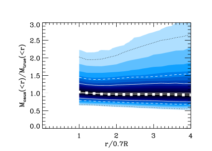
Figure 13: Profiles of the ratio between the caustic and the true mass profile, when combined with the virial masses. The lines and shaded areas are as in Figure 10.

5.4 The gravitational potential profile

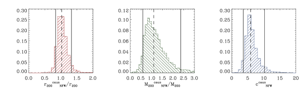
Figure 14: Distribution of the ratio between the parameters of the best NFW fit to the caustic mass profile and the true $M_{200}$ and $r_{200}$ (left and central panels) and distribution of the concentration parameter of the best NFW fit to the caustic mass profile (right panel). The dashed lines indicate the median while the solid lines show the 90 percent range.

Within $r=1h^{-1}$ Mpc, we fit the caustic mass profile of each individual cluster with an NFW profile. The scale factor $r_{200}$ derived from this fit agrees with the true $r_{200}$ derived in 3D; the percentile range of their ratio is $[0.84,1.03,1.33]$. Consequently, for $M_{200}$, which is proportional to $r_{200}^{3}$, we have $[0.59,1.10,2.36]$ (Figure 14).

However, the concentration parameter $c$ derived from the NFW fit to the caustic mass profile tends to overestimate by 36 percent, on average, the concentration parameter of the NFW fit to the 3D mass profile: in fact, the caustic $c$ has percentile range $[3.59,5.92,10.23]$, whereas we find $[2.06,4.62,6.50]$ in 3D; the ratio of these two parameters has percentile range $[0.73,1.36,3.26]$. This result is an obvious consequence of the mass overestimate at small radii (Figure 12).

Figure 15: Left panel: Profiles of the ratio between the NFW gravitational potential profile, with parameters derived from the NFW best fit to the caustic mass profile, and the numerical gravitational potential profile derived from the true mass distribution within $r_{\rm max}=10h^{-1}$ Mpc from the cluster centre. Right panel: Profiles of the ratio between the NFW best fit to the caustic mass profile, and the true mass profile. In both panels, 90 and 50 percent of the profiles are within the upper and lower dotted and solid curves, respectively. The central solid curves are the median profiles. For each cluster, the NFW fit to the mass profile is only performed to the mass distribution within $1h^{-1}$ Mpc.

The NFW fit parameters can be used to derive the gravitational potential profile of the cluster. The left panel of Figure 15 shows that the estimated gravitational potential profile returns the true profile within 10 percent, on average, and, in 50 percent of the cases, the estimated profile is within 25 percent from the real one out to $4r_{200}$. This result is impressive and derives from the mild radial variation of the functions ${\cal F}(r)$ and $g(\beta)$ in hierarchical clustering models.

The right panel of Figure 15 shows the ratio between the caustic mass profile derived from the NFW fit and the true mass profile. The agreement is again good, within 20 percent, although not as good as in Figure 12, because the caustic estimate is biased low due to the overestimate of $c$.

5.5 Uncertainty estimate

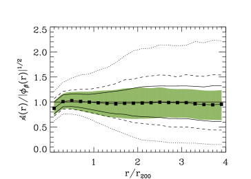
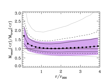
Figure 16: The shaded areas show the median uncertainties estimated from equations (24) and (25). For comparison, we also show the 90 (dotted lines), 68 (dashed lines), and 50 (solid lines) percent ranges of the profiles from Figure 10. The solid squares show the median profiles.

Figures 10 and 12 show the spread derived from the distribution of the profiles of the individual clusters. This spread is mostly due to projection effects, as we will see below (Sect. 6.3). We remind here the simple recipe suggested in D99 to estimate this spread when observing a real cluster of galaxies.

The uncertainty in the measured value of ${\cal A}(r)$ depends on the number of galaxies contributing to the determination of ${\cal A}(r)$; we thus define the relative error

$$\delta{\cal A}(r)/{\cal A}(r)=\kappa/\max\{f_{q}(r,v)\},$$ (24)

where the maximum value of $f_{q}(r,v)$ is along the $v$-axis at fixed $r$. The resulting error on the cumulative mass profile is

$$\delta M_{i}=\sum_{j=1,i}|2m_{j}\delta{\cal A}(r_{j})/{\cal A}(r_{j})|,$$ (25)

where $m_{j}$ is the mass of the shell $[r_{j-1},r_{j}]$ and $i$ is the index of the most external shell.

The shaded bands in Figure 16 are the median spreads derived from the above equations. The median uncertainty on the escape velocity profile increases up to $r\sim 1.5r_{200}$ and remains within $\sim 20-30$ percent at larger radii. The mass profile has a slightly larger uncertainties but remains below $\sim 30-40$ percent out to $r\sim 3r_{200}$. At radii smaller than $\sim 0.6r_{200}$ the assumption of a constant filling function ${\cal F}_{\beta}(r)$ breaks down, as we mentioned above, but this mass overestimate is systematic and can be easily taken into account.

Figure 16 shows that our recipes for the estimate of the uncertainties yield values in good agreement with the 50 percent range of the profiles. Therefore, when applied to real clusters, this algorithm provides uncertainties with 50 percent confidence levels.

6 Systematics

In this section we investigate the systematic errors affecting the estimate of the escape velocity and mass profiles: the systematic errors can originate from the centre location, the parameters of the algorithm, and the projection effects. We also show how the accuracy of the estimate depends on the number of objects in the redshift catalogue.

6.1 Centre identification

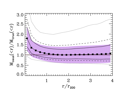
Figure 17: Profiles of the ratio between the caustic and the true mass profile when the centre is forced to be the true one. The lines and shaded areas are as in Figure 16.

In Sect. 5.1, we show how the cluster centre generally is well recovered. The deviations are smaller than $0.07^{\circ}$ on the sky and 250 km s^-1 along the line of sight in 90 percent of the clusters. These deviations produce negligible effects on the mass profile estimate. Figure 17 shows the ratio between the caustic mass profile and the true mass profile, when the centre of the cluster is imposed to be the true one. A comparison with Figure 12 shows that the average profile is still correct at radii larger than $0.6r_{200}$: forcing the method to use the correct centre only slightly improves the estimate and reduces the scatter at radii larger than $\sim 2.5r_{200}$. It is worth pointing out that forcing the code to use the correct centre alters the quantities involved in the construction of the redshift diagram, specifically we recompute the velocity dispersion and the cluster size $R$ of the candidate cluster members with respect to the new centre. We then derive the new redshift diagram and locate the caustics. Despite these variations, the mass profile estimate does not substantially change. This result confirms the robustness of the method.

6.2 Tuning the parameters

Figure 18: Profiles of the ratio between the caustic and the true escape velocity profiles when the parameters are finely tuned (left panel) and from the automatic procedure (right panel) in a subsample of 100 mock catalogues: 50, 68, and 90 percent of the profiles are within the upper and lower solid, dashed, and dotted curves, respectively. The solid squares show the median profiles.

The algorithm allows the user to choose some parameters, namely the thresholds of the binary tree, the optimal smoothing length $h_{c}$ for the galaxy density distribution in the redshift diagram, and the threshold $\kappa$. This freedom is necessary when the target cluster is in particularly crowded regions, or the galaxy sampling is too sparse. In these cases, the algorithm is either unable to locate the caustics or it returns unrealistic caustic amplitudes. If one is interested in the average profiles of a large cluster sample, tuning the caustic parameters for each individual cluster can be very time consuming. To quantify the impact of this possible fine tuning, for each of our 100 simulated clusters, we randomly draw one of the 30 projections and tune the input parameters by hand until the caustic location appears to be close enough to where we might expect them to be by eye. It turns out that most clusters need a rather minor fine tuning, as demonstrated by the final result shown in Figure 18. The left-hand panel shows the caustic amplitude when we apply a fine tuning to the parameters; the right-hand panel is for the same sample without fine tuning. Clearly, the median profile remains unchanged, but the scatter is slightly reduced.

6.3 Projection effects

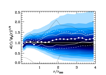
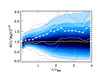
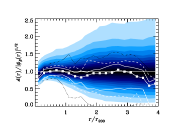
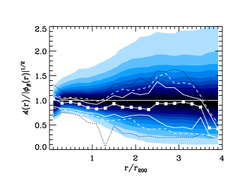
Figure 19: Profiles of the ratio between the caustic amplitude ${\cal A}(r)$ and the l.o.s. component of the true escape velocity $\langle v_{\rm esc,los}^{2}(r)\rangle=-2\phi(r)/g(\beta)\equiv\phi_{\beta}(r)$ for four randomly chosen clusters. The numerical gravitational potential profile $\phi(r)$ is derived from the true mass distribution within $r_{\rm max}=10h^{-1}$ Mpc from the cluster centre: 50, 68, and 90 percent of the profiles derived from 30 different l.o.s. are within the upper and lower solid, dashed, and dotted curves, respectively. The solid squares show the median profiles. The shaded areas are taken from Figure 10.

The analysis provided above clearly shows that the uncertainties on the cluster centre determination and the freedom on the algorithm parameters are not responsible for most of the spread of the escape velocity and mass profiles.

This spread originates from the assumption of spherical symmetry. In hierarchical clustering, this assumption does not hold in general, but observationally our information is limited to the galaxy distribution on the sky alone, although various techniques can in principle provide information on the 3D shape of the cluster (e.g. Zaroubi et al., 2001; Ameglio et al., 2009).

To show the impact of the projection effects on the caustic method, we take our 100 clusters and plot the escape velocity profiles derived from each of the 30 lines of sight. Figure 19 shows four randomly chosen clusters as examples. The caustic technique returns a median profile systematically large for the cluster in the top-right panel. In the other three cases, however, the median profile is within 30 percent of the correct one out to $\sim 3r_{200}$.

The relevant result of this test is the fact that the spread due to the different lines of sight is comparable to the spread of the entire sample (shaded area) taken from Figure 10. This result clearly indicates that the projection effects are the major responsible for the systematic uncertainties of the caustic technique and further refinements of the technique, which still assume spherical symmetry, appear to be unable to improve the mass estimate.

6.4 Dependence of the profiles on the number of particles

Figure 20: Ratio between the estimated and true escape velocity profiles for subsamples with a given number of particles within $3r_{200}$ as indicated in each panel; 50, 68, and 90 percent of the profiles are within the upper and lower solid, dashed, and dotted curves, respectively. The solid squares show the median profiles.

To return a reliable estimate of the escape velocity and mass profiles, the caustic technique requires a sufficient number of redshifts sampling the cluster velocity field.

To quantify this number, we stack our 3000 mock catalogues and apply the caustic technique to the stacked cluster with an increasing number of particles in the catalogue. With this procedure we average over the different lines of sight and the final stacked cluster is very close to be spherically symmetric. We randomly choose particles in the catalogue until we obtain a given number $N$ of particles within $3r_{200}$ from the cluster centre in real space. We consider catalogues with $N=[100,200,350,500,1000,2000]$. We compile 100 different catalogues for each value of $N$. The catalogues with the same $N$ clearly have different total numbers of particles in the catalogue. Table 2 lists the percentile ranges of the total number of particles in the catalogues, which, as usual, have a field of view $12\times 12$ $h^{-2}$ Mpc² at the cluster redshift. Table 2 also lists the total number of particles in a field of view of $30^{\prime}\times 30^{\prime}$ ($2.46\times 2.46$ $h^{-2}$ Mpc²) and $|\Delta v_{\rm los}|\leq 2000$ km s^-1 centred on the cluster.

Figure 20 shows the escape velocity profiles for the six different sets of catalogues. The spread decreases with the increasing number of particles, as expected. However, the profile tends to be overestimated at large radii and with richer catalogues. This result originates from the fact that, as it was already noticed by D99, Schmalzing & Diaferio (2000), and Casagrande & Diaferio (2006), mock redshift surveys extracted from $N$-body simulations show large-scale structures which are less sharp than in the real universe. Therefore, when we increase the number of particles in our mock catalogues, we start sampling the surrounding structure of the cluster in real space, the expected trumpet shape of the particle density distribution in the redshift diagram becomes fuzzier, and the caustic algorithm has increasing difficulty at locating the caustics properly. This problem is not present in real surveys (e.g. Rines & Diaferio, 2006). At these scales, the dark matter particles, that we use here, and the galaxies might not share the same distribution in the redshift diagram and an appropriate galaxy formation algorithm in mock surveys might provide sharper large-scale structures. At any rate, Figure 20 shows that as few as $\sim 200$ galaxies within $3r_{200}$, i.e. a few tens of redshifts per squared comoving megaparsec within the cluster, are sufficient to have a reasonably accurate estimate of the escape velocity profile out to $\sim 4r_{200}$.

Number of particles
within $3r_{200}$	in the catalogue			FOV
$N$	10%	median	90%	10%	median	90%
100	406	470	556	89	98	106
200	841	948	1023	184	194	209
350	1504	1628	1772	326	339	355
500	2162	2327	2477	465	487	506
1000	4497	4693	4887	947	975	1003
2000	9013	9359	9625	1904	1946	1979

Table 2: Number of particles in the catalogues compiled from the stacked cluster. The FOV columns list the numbers of particles within the field of view $30^{\prime}\times 30^{\prime}$ ($2.46\times 2.46$ $h^{-2}$ Mpc²) and $|\Delta v_{\rm los}|\leq 2000$ km s^-1 centred on the cluster.

7 Discussion and conclusion

We use a large sample of galaxy clusters extracted from a cosmological $N$-body simulation to show that, by using galaxy redshifts alone, the caustic technique measures (1) the escape velocity profiles of individual galaxy clusters with 1-$\sigma$ uncertainty between $\sim 20$ and $\sim 50$ percent when the clustrocentric distances increase from $\sim 0.1r_{200}$ to $4r_{200}$, and (2) the cluster mass profiles with $\sim 50$ percent 1-$\sigma$ uncertainty at clustrocentric distances in the range $\sim(0.6-4)r_{200}$. The technique returns reliable estimates when a few tens of redshifts per squared comoving megaparsec within the cluster are available. For sparser samples, the technique can be applied to synthetic clusters obtained by stacking individual clusters. The technique relies on the kinematic properties of galaxy clusters in hierarchical clustering scenarios of structure formation and assumes spherical symmetry. This assumption alone is responsible for most of the estimated uncertainty.

The caustic amplitude measures the profile of the escape velocity along the line of sight, which is a combination of the gravitational potential profile and the velocity anisotropy parameter profile $\beta(r)$. There are extensive attempts to estimate $\beta(r)$ and mass profiles by modelling the density of galaxies in the redshift diagrams with sensible distribution functions (Wojtak et al., 2009; Wojtak & Lokas, 2010). These methods assume dynamical equilibrium and the caustic measure can thus provide a robust consistency check of these estimates of $\beta(r)$ within $r_{200}$.

Cupani et al. (2008) have proposed a new approach, based on the spherical collapse model, to estimate the mass profile of galaxy clusters beyond their virial radius. The spherical collapse model poorly describes the formation of individual clusters in hierarchical clustering scenarios. Nevertheless, Cupani et al. (2008)’s method seems to provide cluster masses with $50$ percent uncertainty on average, once the mean density of the universe $\Omega_{0}$ is set and an appropriate subsample of galaxies is chosen based on their phase-space coordinates (Cupani et al., 2010).

In addition to the caustic method and the Cupani et al. (2008)’s technique, the only method available to estimate the mass of clusters beyond their virial radius is gravitational lensing. However, the lensing signal is strong enough only when the cluster is within the redshift range $z\sim 0.1-1$, whereas, in principle, the caustic technique can be applied to clusters at any redshift and it is only limited by the observing time required to measure a large enough number of galaxy spectra. The caustic technique relies on the assumption that randomly chosen galaxies are fair tracers of the velocity field, whereas gravitational lensing provides a direct measure of the projected mass distribution. All methods based on optical data relies on the absence of velocity bias between galaxies and dark matter, and both $N$-body simulations (e.g. Diaferio et al., 2001; Gill et al., 2004; Diemand et al., 2004; Gill et al., 2005) and observations (e.g. Rines et al., 2008) indicate that this assumption is indeed reasonable. Selected galaxy samples do however have velocity biases: in fact, elliptical galaxies, disk galaxies, and galaxies showing signs of interactions can have substantially different velocity distributions both in observations (e.g. Biviano & Katgert, 2004; Moss, 2006) and in simulated clusters (e.g. Diaferio, 1999).

The caustic technique estimates the escape velocity from a cluster. Therefore, it can also be used to identify the galaxy members of the cluster. This argument is not limited to clusters, and the caustic technique was indeed applied to removing stellar interlopers in dwarf galaxies (Serra et al., 2010) and the Milky Way stellar halo (Brown et al., 2010). The technique arranges the galaxies in the cluster field in a binary tree and a by-product of this analysis is the substructure identification. Here, we have focussed on the estimate of the escape velocity and mass profiles of galaxy clusters. We will investigate the use of the caustic technique to identify members and substructure of self-gravitating systems in future work.

With the advent of the future generation of large spectroscopic surveys, both from ground (e.g., BigBOSS) and from space (e.g., EUCLID), the application of the caustic technique can represent an extremely valuable tool to estimate mass profiles and galaxy membership over a large ensemble of galaxy clusters out to large radii from the cluster centre, thus providing important information on the cosmological assembly of dark matter halos and on the galaxy-environment connection.

References

- Ameglio et al. (2009) Ameglio S., Borgani S., Pierpaoli E., Dolag K., Ettori S., Morandi A., 2009, MNRAS, 394, 479
- Andersson et al. (2010) Andersson K., et al., 2010, ArXiv e-prints: 1006.3068
- Andreon & Hurn (2010) Andreon S., Hurn M. A., 2010, MNRAS, 404, 1922
- Biviano (2006) Biviano A., 2006, ArXiv e-prints: 0607040
- Biviano & Girardi (2003) Biviano A., Girardi M., 2003, ApJ, 585, 205
- Biviano & Katgert (2004) Biviano A., Katgert P., 2004, A&A, 424, 779
- Borgani (2006) Borgani S., 2006, ArXiv e-prints: 0605575
- Borgani et al. (2004) Borgani S., et al., 2004, MNRAS, 348, 1078
- Brown et al. (2010) Brown W. R., Geller M. J., Kenyon S. J., Diaferio A., 2010, AJ, 139, 59
- Casagrande & Diaferio (2006) Casagrande L., Diaferio A., 2006, MNRAS, 373, 179
- Colless et al. (2001) Colless M., et al., 2001, MNRAS, 328, 1039
- Cupani et al. (2008) Cupani G., Mezzetti M., Mardirossian F., 2008, MNRAS, 390, 645
- Cupani et al. (2010) —, 2010, MNRAS, 403, 838
- Czoske et al. (2002) Czoske O., Moore B., Kneib J.-P., Soucail G., 2002, A&A, 386, 31
- Diaferio (1999) Diaferio A., 1999, MNRAS, 309, 610
- Diaferio (2009) —, 2009, ArXiv e-prints: 0901.0868
- Diaferio et al. (2005a) Diaferio A., et al., 2005a, MNRAS, 356, 1477
- Diaferio & Geller (1997) Diaferio A., Geller M. J., 1997, ApJ, 481, 633
- Diaferio et al. (2005b) Diaferio A., Geller M. J., Rines K. J., 2005b, ApJ, 628, L97
- Diaferio et al. (2001) Diaferio A., Kauffmann G., Balogh M. L., White S. D. M., Schade D., Ellingson E., 2001, MNRAS, 323, 999
- Diaferio et al. (2008) Diaferio A., Schindler S., Dolag K., 2008, Space Science Reviews, 134, 7
- Diemand et al. (2004) Diemand J., Moore B., Stadel J., 2004, MNRAS, 352, 535
- Domínguez et al. (2001) Domínguez M., Muriel H., Lambas D. G., 2001, AJ, 121, 1266
- Drinkwater et al. (2001) Drinkwater M. J., Gregg M. D., Colless M., 2001, ApJ, 548, L139
- Dunkley et al. (2009) Dunkley J., et al., 2009, ApJ Supplements, 180, 306
- Geller et al. (1999) Geller M. J., Diaferio A., Kurtz M. J., 1999, ApJ, 517, L23
- Gill et al. (2005) Gill S. P. D., Knebe A., Gibson B. K., 2005, MNRAS, 356, 1327
- Gill et al. (2004) Gill S. P. D., Knebe A., Gibson B. K., Dopita M. A., 2004, MNRAS, 351, 410
- Heisler et al. (1985) Heisler J., Tremaine S., Bahcall J. N., 1985, ApJ, 298, 8
- Hiotelis (2001) Hiotelis N., 2001, A&A, 375, 338
- Huertas-Company et al. (2009) Huertas-Company M., Foex G., Soucail G., Pelló R., 2009, A&A, 505, 83
- Kneib et al. (2003) Kneib J.-P., et al., 2003, ApJ, 598, 804
- Lemze et al. (2009) Lemze D., Broadhurst T., Rephaeli Y., Barkana R., Umetsu K., 2009, ApJ, 701, 1336
- Mahdavi et al. (1999) Mahdavi A., Geller M. J., Böhringer H., Kurtz M. J., Ramella M., 1999, ApJ, 518, 69
- Martínez et al. (2008) Martínez H. J., Coenda V., Muriel H., 2008, MNRAS, 391, 585
- Materne (1978) Materne J., 1978, A&A, 63, 401
- Merritt (1987) Merritt D., 1987, ApJ, 313, 121
- Moss (2006) Moss C., 2006, MNRAS, 373, 167
- Motl et al. (2005) Motl P. M., Hallman E. J., Burns J. O., Norman M. L., 2005, ApJ, 623, L63
- Nagai (2006) Nagai D., 2006, ApJ, 650, 538
- Nagai et al. (2007) Nagai D., Vikhlinin A., Kravtsov A. V., 2007, ApJ, 655, 98
- Navarro et al. (1997) Navarro J. F., Frenk C. S., White S. D. M., 1997, ApJ, 490, 493
- Peebles (1993) Peebles P. J. E., 1993, Principles of physical cosmology. Princeton Series in Physics, Princeton, NJ: Princeton University Press
- Pierpaoli et al. (2003) Pierpaoli E., Borgani S., Scott D., White M., 2003, MNRAS, 342, 163
- Piffaretti & Valdarnini (2008) Piffaretti R., Valdarnini R., 2008, A&A, 491, 71
- Proust et al. (2006) Proust D., et al., 2006, A&A, 447, 133
- Rasia et al. (2006) Rasia E., et al., 2006, MNRAS, 369, 2013
- Regös & Geller (1989) Regös E., Geller M. J., 1989, AJ, 98, 755
- Reisenegger et al. (2000) Reisenegger A., Quintana H., Carrasco E. R., Maze J., 2000, AJ, 120, 523
- Rines & Diaferio (2006) Rines K., Diaferio A., 2006, AJ, 132, 1275
- Rines & Diaferio (2010) —, 2010, AJ, 139, 580
- Rines et al. (2007) Rines K., Diaferio A., Natarajan P., 2007, ApJ, 657, 183
- Rines et al. (2008) —, 2008, ApJ, 679, L1
- Rines et al. (2010) Rines K., Geller M. J., Diaferio A., 2010, ApJ, 715, L180
- Rines et al. (2002) Rines K., Geller M. J., Diaferio A., Mahdavi A., Mohr J. J., Wegner G., 2002, AJ, 124, 1266
- Rines et al. (2003) Rines K., Geller M. J., Kurtz M. J., Diaferio A., 2003, AJ, 126, 2152
- Sarazin (1988) Sarazin C. L., 1988, X-ray emission from clusters of galaxies. Cambridge Astrophysics Series, Cambridge: Cambridge University Press, 1988
- Schmalzing & Diaferio (2000) Schmalzing J., Diaferio A., 2000, MNRAS, 312, 638
- Schneider (2006) Schneider P., 2006, in Saas-Fee Advanced Course 33: Gravitational Lensing: Strong, Weak and Micro, Meylan G., Jetzer P., North P., Schneider P., Kochanek C. S., Wambsganss J., eds., pp. 1–89
- Serna & Gerbal (1996) Serna A., Gerbal D., 1996, A&A, 309, 65
- Serra et al. (2010) Serra A. L., Angus G. W., Diaferio A., 2010, ArXiv e-prints: 0907.3691
- Silverman (1986) Silverman B. W., 1986, Density estimation for statistics and data analysis. Monographs on Statistics and Applied Probability, London: Chapman and Hall, 1986
- Skibba et al. (2009) Skibba R. A., et al., 2009, MNRAS, 399, 966
- Springel et al. (2001) Springel V., Yoshida N., White S. D. M., 2001, New Astronomy, 6, 79
- The & White (1986) The L. S., White S. D. M., 1986, AJ, 92, 1248
- van Haarlem & van de Weygaert (1993) van Haarlem M., van de Weygaert R., 1993, ApJ, 418, 544
- Voit (2005) Voit G. M., 2005, Reviews of Modern Physics, 77, 207
- White et al. (2010) White M., Cohn J. D., Smit R., 2010, MNRAS, 408, 1818
- Wojtak & Lokas (2010) Wojtak R., Lokas E. L., 2010, ArXiv e-prints: 1004.3771
- Wojtak et al. (2009) Wojtak R., Łokas E. L., Mamon G. A., Gottlöber S., 2009, MNRAS, 399, 812
- Zaroubi et al. (2001) Zaroubi S., Squires G., de Gasperis G., Evrard A. E., Hoffman Y., Silk J., 2001, ApJ, 561, 600
- Zwicky (1937) Zwicky F., 1937, ApJ, 86, 217