Goal-oriented A Posteriori Error Estimation for Finite Volume Methods

Abstract

A general framework for goal-oriented a posteriori error estimation for finite volume methods is presented. The framework does not rely on recasting finite volume methods as special cases of finite element methods, but instead directly determines error estimators from the discretized finite volume equations. Thus, the framework can be applied to arbitrary finite volume methods. It also provides the proper functional settings to address well-posedness issues for the primal and adjoint problems. Numerical results are presented to illustrate the validity and effectiveness of the a posteriori error estimates and their applicability to adaptive mesh refinement.

1 Introduction

Finite volume methods have become increasingly popular due to their intrinsic conservative properties and their capability in dealing with complex domains; see, e.g. [11, 15]. Hence, a posteriori error estimates for finite volume methods are important as they aid in error control and improve the overall accuracy of numerical simulations. A posteriori error estimates also play a key role in the implementation of adaptive mesh refinement methods. In fact, the main motivation of the current work is to find simple and robust a posteriori error estimators to guide adaptive mesh refinements for finite volume methods in regional climate modeling [7, 16].

The literature on a posteriori error analysis for finite volume methods is slim compared to that for finite element methods. A large part of the available works aim to derive a posteriori error bounds for approximate solutions in certain global energy norms; see, e.g. [1, 2, 3, 5, 12, 13, 18, 19].

We are particularly interested in another type of a posteriori error estimates that are goal oriented, i.e., estimates of errors in certain quantities of interest. A goal-oriented error estimate is potentially very useful in assisting in error control. However, the literature on goal-oriented a posteriori error estimates for finite volume methods is even scarcer, probably due to the fact that finite volume methods do not naturally fit into variational frameworks. Insightful efforts have been made to address this challenge by exploiting the equivalence between certain finite volume methods and numerical schemes in variational forms such as the finite element methods or discontinuous Galerkin methods. For example, in [4], a goal-oriented a posteriori error estimate is presented for a special type of finite volume method that is equivalent to a Petrov-Galerkin variant of the discontinuous Galerkin method. In [9], an a posteriori error analysis is presented for cell-centered finite volume methods for the convection-diffusion problem by utilizing the equivalence between the finite volume methods and the lowest-order Raviart-Thomas mixed finite element method with a special quadrature. However, the applicability of this approach is limited for two reasons. First, on many grids on which finite volume schemes are constructed, there are no quadrature rules known, and thus implementing finite element or discontinuous Galerkin schemes on these grids is impractical. An example of such grids is hexagonal Voronoi grid ([DFGun99]). The other reason is that finite volume methods for real-world problems are often sophisticated in themselves, and it is often not clear, to say the least, how to establish a connection to schemes in variational forms. In this regard we again refer to [15].

In this work, we aim to derive a general functional analytic framework for a posteriori error estimation for arbitrary finite volume methods. The idea is to derive a posteriori error estimators at the partial differential equation level in an appropriate functional setting. This approach does not require the differential equations or the numerical schemes to be recast in variational form nor do they rely on connecting an finite volume method with a finite element method. The approximate solutions produced by finite volume methods are simply taken as inputs to the a posteriori error estimator. Because the a posteriori error estimation is independent of the exact form of the finite volume method, it can be applied to arbitrary finite volume methods.

In Galerkin finite element or discontinuous Galerkin methods, the difference $u-u_{h}$ between the exact solution $u$ and the approximate solution $u_{h}$ is orthogonal to the test function space $V_{h}$. For this reason, a posteriori error estimation for these methods requires that the adjoint solution $\phi$ be sought in a space $V_{h^{\prime}}$ larger than $V_{h}$. This restriction does not apply in our approach due to the very fact that finite volume schemes do not naturally fit into variational forms, though for the sake of accuracy, it may be advantageous to seek the adjoint solution with a higher order scheme. This point will be made clear in the next section.

It has been pointed out that the well-posedness issue for the adjoint equation remains challenging and open in many cases; see, e.g., [4]. A byproduct of our approach is that, because the adjoint problem is naturally posed in an appropriate functional setting, its well posedness can be dealt with by the abundant analytical tools of standard partial differential equation theories; again, see [4].

The rest of the paper is organized as follows. At the beginning of the next section, we present our approach for a posteriori error estimation for finite volume methods in a general functional analytical framework. It is followed by a numerical example demonstrating the error estimates. In Section 3, we present an application of the a posteriori error estimation to adaptive mesh refinement. We conclude with some remarks in Section 4.

2 A posteriori error estimates for finite volume methods

2.1 Abstract framework

Let $H$ denote a Hilbert space endowed with the norm $||\cdot||$ and inner product $(\cdot,\cdot)$. Let $L$ denote an unbounded operator in $H$ with domain $D(L)$ dense in $H$. The primal problem we deal with is succinctly formulated in this functional setting as:
for each $f\in H$, find $\boldsymbol{u}\in D(L)$ such that

$$L\boldsymbol{u}=f.$$ (1)

We consider time-dependent problems so that the operator $L$ usually takes the form

$$L=\dfrac{\partial}{\partial t}+A,$$

where $A$ represents a linear differential spatial operator that is usually also unbounded in a respective function space. In this work, we assume that the primal problem (1) is well-posed, i.e., it possesses a unique solution.

The quantity of interest is given as a possibly nonlinear functional $Q(\boldsymbol{u})$ of $\boldsymbol{u}$. Let $\boldsymbol{u}^{\#}$ denote an approximate solution of the primal problem (1). Then, the error in the quantity of interest can be written as

$$Q(\boldsymbol{u})-Q(\boldsymbol{u}^{\#})=(\boldsymbol{u}-\boldsymbol{u}^{\#},\phi)$$ (2)

for some kernel function $\phi\in H$. We note that the kernel function $\phi$ may depend on $\boldsymbol{u}$; indeed this is the case when $Q$ is a nonlinear function of $u$; see Section 3.

The foregoing assumption that the domain $D(L)$ is dense in $H$ is crucial as it allows us to rigorously define the adjoint operator $L^{*}$ of $L$ and its domain $D(L^{*})$. Indeed, according to [17], a function $\widetilde{\boldsymbol{u}}\in H$ belongs to $D(L^{*})$ if and only if the mapping $D(L):\boldsymbol{u}\longrightarrow(L\boldsymbol{u},\,\widetilde{\boldsymbol{u}})$ is a linear bounded functional on $D(L)$ for the norm of $H$. Because $D(L)$ is dense in $H$, the Hahn-Banach theorem guarantees that the bounded linear functional can be extended to the whole of $H$. Then, by the Riesz representation theorem, there exists a unique element, denoted as $L^{*}\widetilde{\boldsymbol{u}}$, of $H$ such that

$$(L\boldsymbol{u},\,\widetilde{\boldsymbol{u}})=(\boldsymbol{u},\,L^{*}\widetilde{\boldsymbol{u}})\qquad\forall\,\boldsymbol{u}\in D(L).$$ (3)

Thus, $L^{*}$ is a linear, possibly unbounded, operator from $D(L^{*})$ to $H$. The adjoint problem can be formally stated as:
for a given function $\phi\in H$, find $\widetilde{\boldsymbol{u}}\in D(L^{*})$ such that

$$L^{*}\widetilde{\boldsymbol{u}}=\phi.$$ (4)

We will demonstrate, through examples, how to compute adjoint operators. Generally speaking, for time-dependent problems, the operator $L^{*}$ usually has the form of

$$L^{*}=-\dfrac{\partial}{\partial t}-B.$$

Primal time-dependent problems are usually initial-boundary value problems. Consequently, most adjoint problems are final-boundary value problem because the values of the unknown function are imposed at the final time $t=T$. Applying the change of variable $\tau=T-t$ transforms the final-value problem into an initial-value problem. In this way, many analytic techniques can be employed to establish the well-posedness of the adjoint problem. We will demonstrate this point with specific examples.

Now that all the necessary functional settings have been introduced, we shall derive an a posteriori error estimate for the forward problem (1), regardless of the finite volume methods actually used to solve the primal and adjoint problems. By (2)–(4), we infer that

$$Q(\boldsymbol{u})-Q(\boldsymbol{u}^{\#})= (\boldsymbol{u}-\boldsymbol{u}^{\#},\,\phi)$$

$$= (\boldsymbol{u}-\boldsymbol{u}^{\#},\,L^{*}\widetilde{\boldsymbol{u}})$$

$$= (L(\boldsymbol{u}-\boldsymbol{u}^{\#}),\,\widetilde{\boldsymbol{u}})$$

$$= (f-L\boldsymbol{u}^{\#},\,\widetilde{\boldsymbol{u}}).$$

Therefore, we have

$$Q(\boldsymbol{u})-Q(\boldsymbol{u}^{\#})=(f-L\boldsymbol{u}^{\#},\,\widetilde{\boldsymbol{u}}).$$ (5)

Note that the true solution $\boldsymbol{u}$ is not required for computing the error and that, if the adjoint solution $\widetilde{\boldsymbol{u}}$ is exact, then the error estimate is actually exact as well. These are the key advantages of the a posteriori estimate (5). The cost incurred is, of course, the need to solve the adjoint problem (4).

So far we have not discussed the exact form of the finite volume methods. The approximate solutions produced by these schemes are taken as input to (5). Hence, the formula, in principle, applies to arbitrary finite volume methods. We should also note that the approximate solution to the primal problem is usually given in a discrete form and thus the term $L\boldsymbol{u}^{\#}$ in (5) is not well defined at this point. We will explore a walk-around to this issue when we deal with specific examples in Section 2.2 and 3.

2.2 Numerical demonstration: one-dimensional scalar equation

The primary goal of this section is, by the means of a simple example, to demonstrate the implementation of the abstract framework laid out in the previous section. We will also demonstrate the validity of the a posteriori error estimates by comparing the estimated errors with the true errors. Finally, we will explore the impact of the numerical errors in the adjoint solution on a posteriori error estimates, and what measures can be taken to ensure accuracy.

We consider the one-dimensional linear transport equation

$$u_{t}+au_{x}=f, 0<x<1,t>0,$$ (6)

$$u(0,t)=g(t), t>0,$$ (7)

$$u(x,0)=u_{0}(x), 0<x<1.$$ (8)

We assume that the coefficient $a$ is positive and constant, in which case the initial and boundary value problem (6)–(8) is well-posed, provided that the problem is cast in an appropriate functional setting. The well-posedness of this problem will not be discussed here because it is a classical example in partial differential equation theory; see, among many texts, [10]. Nevertheless, we shall specify the proper functional settings for the problem so that its adjoint problem can be defined and an a posteriori error estimate for its solution can be derived.

We let $H=L^{2}\left((0,1)\times(0,T)\right)$ and let $L$ be the linear operator associated with (6)– (8). We define the domain $D(L)$ as

$$\mathcal{D}(L)=\left\{u\in H\,\,|\,\,u_{t}+au_{x}\in H,\,u(0,t)=0,\,u(x,0)=0\right\}.$$

It can shown that $D(L)$ is dense in $H$. For each $u\in\mathcal{D}(L)$, the operator $L$ is defined as

$$Lu=u_{t}+au_{x}.$$

We now define the adjoint operator $L^{*}$ of $L$ and its domain $\mathcal{D}(L^{*})$. We recall that the domain $\mathcal{D}(L^{*})$ is defined as a space of functions $\widetilde{u}$ for which $(Lu,\widetilde{u})$ is a continuous functional for $u\in\mathcal{D}(L)$ with respect to the norm of $H$, that is,

$$\widetilde{u}\in\mathcal{D}(L^{*})\iff u\rightarrow(Lu,\widetilde{u})\textrm{ is continuous in the $H$ norm.}$$

Based on this definition, we determine that $\mathcal{D}(L^{*})$ is given by

$$\mathcal{D}(L^{*})=\left\{\widetilde{u}\in H\,\,|\,\,\widetilde{u}_{t}+a\widetilde{u}_{x}\in H,\,\widetilde{u}(1,t)=0,\,\widetilde{u}(x,T)=0\right\}$$

and, for each $\widetilde{u}\in\mathcal{D}(L^{*})$, we have

$$L^{*}\widetilde{u}=-\widetilde{u}_{t}-a\widetilde{u}_{x}.$$

For $u\in\mathcal{D}(L)$ and $\widetilde{u}\in\mathcal{D}(L^{*})$, the following important relationship holds:

$$(Lu,\,\widetilde{u})=(u,\,L^{*}\widetilde{u}).$$ (9)

Within this functional setting, the adjoint problem can be stated as follows:
for any $\phi\in H$, find $\widetilde{u}\in D(L^{*})$ such that

$$L^{*}\widetilde{u}=\phi.$$ (10)

We now consider the well-posedness issue for the adjoint problem (10). The equations of this problem, in differential form, read

$$-\widetilde{u}_{t}-a\widetilde{u}_{x} =\phi\qquad\textrm{ for }0<x<1,\,\,0<t<T,$$ (11)

$$\widetilde{u}(x,T) =0\qquad\textrm{ for }0<x<1,$$ (12)

$$\widetilde{u}(1,t) =0\qquad\textrm{ for }0<t<T.$$ (13)

The conditions (12) and (13) are due to the requirement that $v$ should be sought in the adjoint domain $\mathcal{D}(L^{*})$. The system (11)–(13) needs to be solved backward in time because a final condition is given at $t=T$. To overcome this awkwardness, we make the change of variable $t=T-\tau.$ Then, the system (11)–(13) becomes

$$\widetilde{u}_{\tau}-a\widetilde{u}_{x}=\phi,$$ (14)

$$\widetilde{u}(x,0)=0,$$ (15)

$$\widetilde{u}(1,\tau)=0,$$ (16)

which can be solved forwards in time. The well-posedness of this system can be studied in the same way as that for the primal system (6)–(8), e.g., by semigroup theory. In the language of that theory, the operator $L^{*}$ is the infinitesimal generator a semigroup of contractions $S(\tau)$. The well-posedness result for the system above is stated in the following theorem.

Theorem 2.1.

If $\phi\in L^{1}(0,T;L^{2}(0,1))$, then there exists an unique solution $\widetilde{u}\in C([0,T];L^{2}(0,1))$ of (14)–(16) of the form

$$\widetilde{u}(\tau)=\int_{0}^{\tau}S(\tau-s)\phi(s)\,\mathrm{d}s.$$

We do not prove the theorem here and instead refer to [14].

The simple example considered in this section demonstrates a key advantage of our approach: we derive and use an adjoint system whose well-posedness can be studied in the same manner as that for the primal system, for which a multitude of analytical tools are available.

We now concern ourselves with linear quantities of interest that can be expressed as

$$Q(u)=\int_{\Omega}u\phi,$$ (17)

where $\phi$ is a kernel function independent of the unknown $u$. Identifying $\phi$ in (17) with $\phi$ in (14), the a posteriori error estimate of $Q(u)-Q(u^{\#})$ is then given by (5). However, there is an implementation issue associated with (5). In practice, we only have the approximate solution $u^{\#}$ in its discrete form, e.g., as approximations of the function values at discrete grid points. For (5) to make sense, we could either define a discrete analogue ${L}^{\#}$ of ${L}$ or define and apply a mapping that maps $u^{\#}$ from its discrete representation to a continuous representation so that the differential operator ${L}$ can be applied. In this work, we take a third approach. We find a way to transpose $L$ back onto $\widetilde{u}$ and then use (10) to replace $L^{*}\widetilde{u}$ by $\phi$. This approach avoids approximating $Lu^{\#}$ with discrete values which usually introduces another source of error. However, we note that, in general, $u^{\#}$ does not belong to $\mathcal{D}(L)$ so that we cannot invoke (9) for $(Lu^{\#},v)$. Thus, we proceed by integration by parts:

$$(Lu^{\#},v) =\int_{I}(u^{\#}_{t}+au^{\#}_{x})v$$

$$=-\int_{t=0}u^{\#}v-a\int_{x=0}u^{\#}v+(u^{\#},\phi).$$

Therefore,

$$Q(u)-Q(u^{\#})=(f,v)-(u^{\#},\phi)+\int_{t=0}u_{0}v+a\int_{x=0}gv.$$ (18)

2.2.1 Numerical results

The forward problem (6)–(8) is solved with the first-order explicit upwind method. The exact form of the scheme is not essential to this work, but we shall briefly state the method for the sake of reference. (Other finite volume methods used in the sequel, however, will not be explicitly described.) We choose $0=x_{0}<x_{1}<\cdots<x_{M}=1$ and let $K_{i}=[x_{i-1},\,x_{i}]$ denote the $i^{\textrm{th}}$ control volume/cell. Obviously, $\{K_{i}\}_{i=1}^{M}$ forms a partition of the interval $[0,1]$. We also set $\Delta t=T/N$ and let $t_{n}=n\Delta t$ denote the discrete time steps. We let $U^{n}_{i}$ denote the average of the unknown $u$ over the cell $K_{i}$ at time $t=t^{n}$. Then, the first-order explicit upwind method for (6) can be written as

$$\dfrac{U^{n+1}_{i}-U^{n}_{i}}{\Delta t}+a\dfrac{U^{n}_{i}-U^{n}_{i-1}}{\delta_{i}}=F^{n}_{i}\quad\textrm{ for }1\leq i\leq M.$$

In the above, $\delta_{i}=|K_{i}|$ and $U_{0}$ is the average of the unknown $u$ on an artificial cell $K_{0}=[x_{-1},\,x_{0}]$ with $x_{-1}=-x_{1}$. The boundary condition (7) can be imposed as

$$\dfrac{1}{2}\left(U^{n+1}_{0}+U^{n+1}_{1}\right)=\dfrac{1}{2}g(t^{n}).$$

To demonstrate the validity of the a posteriori error estimate (18) for the problem (6)–(8), we consider an example with a sine wave solution:

$$u_{t}+u_{x}=0,\qquad 0<x<1,\,0<t<0.5,$$ (19)

$$u(x,0)=\sin(2\pi x),$$ (20)

$$u(0,t)=-\sin(2a\pi t).$$ (21)

This problem has an analytic solution

$$u(x,t)=\sin(2\pi(x-at)),$$ (22)

which allows us to study the performance of the a posteriori error estimate (18) by comparing the estimated errors to the true errors.

For the kernel function $\phi$ in (17), we first consider the simple case

$$\phi=1.$$ (23)

This choice of kernel function emphasizes the accuracy of the solution everywhere in the spatial-temporal region $[0,\,1]\times[0,\,T]$. With this choice of kernel function, we compute the solution on an array of uniform grids, from a coarse one with $M=20*2^{0}$ cells to a fine one with $M=20*2^{4}$ cells. Because the solution of (19)–(21) is just the sine wave given by (22), we can compute the true error in the quantity of interest $Q(u)=\int_{\Omega}u\,\mathrm{d}x\,\mathrm{d}t$. We also compute the solution of the adjoint equation, using the same first-order upwind method, on another array of uniform grids, from a coarse one with $M_{adj}=20*2^{0}$ to a fine one with $M_{adj}=20*2^{3}$. With each of these approximate adjoint solutions, we compute an a posteriori estimate of the error in the quantity of interest using (18). Then we plot the errors in the quantity of interest against the number of grid cells $M$ in Fig. 1.

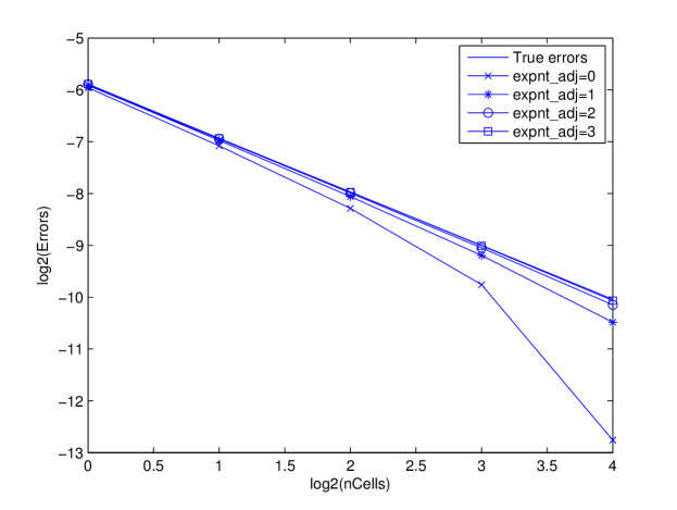
Figure 1: For the simple kernel function $\phi=1$, the errors in the quantity of interest for different grids for the primal and adjoint approximations. The same first-order method is used for discretizing the primal and adjoint equations.

For this simple case, solving the adjoint equation with the same first-order upwind method on a grid that is at most as fine as the grid for the primal equation proves adequate. In fact, with $M_{adj}=20*2^{3}$ (one level coarser than the finest grid for solving the primal equation), the a posteriori error estimates are indistinguishable from the true errors.

However, with a more challenging kernel function, solving the adjoint equation with a numerical method of the same order on a grid with similar resolution may not be adequate. In such cases, increasing the grid resolution for the adjoint equation can solve this difficulty. A more effective solution strategy is to use a higher-order method for the adjoint equation. We demonstrate these observations with the choice

$$\phi=\dfrac{1}{\pi\epsilon^{2}}\exp(-\dfrac{(x-L/2)^{2}+(t-T/2)^{2}}{\epsilon^{2}}).$$ (24)

This kernel function emphasizes the accuracy of the solution in a small region of radius $\epsilon$ surrounding the point $(x=L/2,t=T/2)$ in the space-time computational domain.

We first solve the adjoint equation with the same first-order upwind method as used for the primal problem on an array of uniform grids with increasing resolutions. The results are presented in Fig. 2.

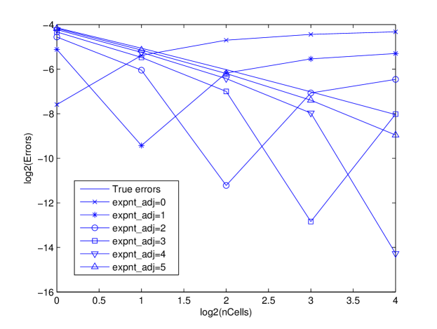
Figure 2: For the kernel function (24), the errors in the quantity of interest for different grids for the primal and adjoint approximations. The same first-order method is used for discretizing the primal and adjoint equations.

What we see is that on coarse grids (in this case $M_{adj}=20*2^{q}$ with $q=0,\,1,\,2,\,3$), the adjoint solutions are not accurate enough to produce sensible estimates of the errors in the quantity of interest. We also see that with increasing resolutions for the adjoint approximation, the a posteriori estimates of the errors are converging to the true errors. In fact, at $M_{adj}=20*2^{5}$, the errors estimates can be regarded as decent approximations of the true errors.

Next, we change our strategy, and solve the adjoint equation using the leap-frog method which is second-order accurate both in time and space. The results are shown in Fig. 3.

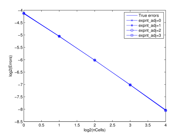
Figure 3: For the kernel function (24), the errors in the quantity of interest for different grids for the primal and adjoint approximations. A higher-order method is used for discretizing the adjoint equations compared to that used for the primal equations.

The leap-frog method provides a very efficient solution. In fact, even on the coarsest grid with just $M_{adj}=20$, the adjoint solution is accurate enough to produce error estimates that are indistinguishable from the true errors.

In the Galerkin–type variational approach towards a posteriori error estimation for finite volume schemes ([4, 9]), it is required that the solution of the adjoint problem be sought in a function space larger than the solution space for the primal problem, due to the orthogonality between the residual and the test function space. This requirement does not apply to our approach, because neither of the finite volume schemes for the primal or adjoint problems is based on variational formulations. In fact, for the cases (23) and (24) considered in this section, both the primal and adjoint problems are solved in piecewise constant function spaces, so to speak. The more complex case (24) poses some challenges because the errors in the adjoint solution starts to deteriorate the a posteriori estimates of the errors in the quantity of interest corresponding to this kernel function. Solving the adjoint problem in a broader function space, e.g. by implementing a Godunov-type higher-order finite volume scheme ([4, Lev02]), is certainly a possible strategy. This strategy is not explored in this work. Instead, we demonstrate through numerical results that the challenges can also be met, to various extents, solely by refining the mesh or implementing a plain high order scheme (e.g. from a first-order upwind scheme to a second-order leap-frog scheme). The function spaces for the solutions of the adjoint problems remain piecewise constant.

3 Application to adaptive mesh refinement for the 1D shallow water equations

In this section, we demonstrate the application of the a priori error estimate, derived in Section 2.1, to adaptive mesh refinement for finite volume methods. We take the system of one dimensional linearized shallow water equations as an example. We also discuss the challenge and the handling of a nonlinear quantity of interest.

3.1 Types of adaptive mesh refinement strategies

We can identify the following types of adaptive mesh refinement strategies:

Type 1.

Time unvarying adaptive mesh refinement.
The mesh for the spatial dimensions is adaptively refined, but remains fixed for the whole simulation period. The time steps are non-adaptive, though they could be nonuniform. A generic depiction of the resulting grid is given in Fig. 4.

Type 2.

Non-incremental time varying adaptive mesh refinement.
The spatial mesh is adaptively refined for each temporal sub-interval of the simulation. The time step is non-adaptive, though it could be nonuniform. The mesh refinement is done after each full simulation, i.e., not incrementally in time. A generic depiction of the resulting grid is given in Fig. 5

Type 3.

Incremental time varying adaptive mesh refinement.
The spatial mesh is adaptively refined at each sub-interval of the simulation period, as the simulation proceeds. The time step is non-adaptive, though it could be nonuniform.

Type 4.

Incremental time varying adaptive mesh with adaptive time steps.

In this article, we discuss the Type 1 and 2 strategies and leave the more sophisticated Type 3 and 4 strategies to future work.

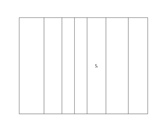
Figure 4: Sketch of a Type 1 adaptively refined mesh.

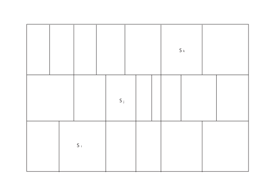
Figure 5: Sketch of a Type 2 adaptively refined mesh.

The elegant formula (5) cannot be applied directly for adaptive mesh refinements because it does not provide information about local errors. In order to obtain such information, we need to break down the whole space-time domain into slabs, and find a means for calculating the error contribution from each slab. We note that each slab can contain one or more of the time steps used to for discretization of the partial differential equations. Let $\{t_{j}\}_{j=0}^{N}$ be a partition of the whole simulation period $[0,\,T]$, and for each $j$, let $\{K_{ij}\}_{i=1}^{M_{j}}$ be a partition of the spatial domain $(0,\,1)$ during the time period $[t_{j-1},t_{j}]$. Then each slab $S_{ij}$ is given by

$$S_{ij}=K_{ij}\times t_{j}.$$

We note that this partition of the space-time domain can accommodate the Type 1 adaptive mesh refinement strategy with $N=1$; see Fig. 4. With $N>1$, it can accommodate the adaptive mesh refinement strategies of Type 2 as well as of Type 3 and 4; see Fig. 5.

By (5),

$$Q(u)-Q(\boldsymbol{u}^{\#}) =(f-L\boldsymbol{u}^{\#},\widetilde{\boldsymbol{u}})$$

$$=\int_{I}(f-L\boldsymbol{u}^{\#})\widetilde{\boldsymbol{u}}\,\mathrm{d}x\,\mathrm{d}t$$

$$=\sum\int_{S_{ij}}(f-L\boldsymbol{u}^{\#})\widetilde{\boldsymbol{u}}\,\mathrm{d}x\,\mathrm{d}t$$

$$=\sum_{i,j}E_{ij},$$

where

$$E_{ij}=\int_{S_{ij}}(f-L\boldsymbol{u}^{\#})\widetilde{\boldsymbol{u}}\,\mathrm{d}x\,\mathrm{d}t$$

denoting the error contribution from each slab $S_{ij}$.

Below is a simple adaptive mesh refinement algorithm based on the error contribution from each slab:

⬇

Step 0. Specify the total error tolerance TOL.

Step 1. Calculate E_ij for each i and j.

Step 2. Calculate Total_error = sum of E_ij

Step 3. If Total_error >= TOL, then

For 1 <= j <= N, 1 <= i <= M_j

If |E_ij| >= TOL/M then

Refine the grid over the cell K_ij

End

End

Goto Step 1.

Else if Total_error < TOL, then

Exit

End

We note that this adaptive mesh refinement algorithm usually leads to over refinement because it does not account for the error cancellations among grid cells. Nevertheless, it is adequate for our purpose to demonstrate the application of the a posteriori error estimate (5) to adaptive mesh refinement for finite volume methods. For more discussions on adaptive mesh refinement algorithms, see, e.g. [8].

3.2 1D shallow water equations

We now apply the a posteriori error estimate (5) to adaptive mesh refinement for the one-dimensional, linearized shallow water system

$$\left\{\begin{aligned} &\dfrac{\partial h}{\partial t}+h_{x}+u_{x}=0,\\ &\dfrac{\partial u}{\partial t}+2h_{x}+u_{x}=0.\end{aligned}\right.$$ (25)

We remark that, among many things, the shallow water system can be used to model tsunami waves. In (25), the system has been non-dimensionalized, coefficients involving physical quantities have be replaced by somewhat artificial constants, and the mathematically non-essential Coriolis forcing terms have been omitted, all for the sake of simplicity. Despite these heavy simplifications, the system (25) still retains some interesting physical features, e.g. gravity waves (the underlying mechanism of tsunamis [P87, Maj03]), and therefore is adequate for the purpose of this section.

The coefficient matrix of the system (25), given by

$$\left(\begin{aligned} &1&1\\ &2&1\end{aligned}\right),$$

has two eigenvalues

$$\lambda_{+}=1+\sqrt{2}>0\qquad\mbox{and}\qquad\lambda_{-}=1-\sqrt{2}<0.$$

The system is sometimes referred to as the subcritical mode of the primitive equations due to the the opposite signs of the eigenvalues. For a discussion on a related problem, see [6]. The eigenvectors of the coefficient matrix form a transformation matrix $P$ such that

$$P^{-1}\left(\begin{aligned} &1&&1\\ &2&&1\end{aligned}\right)P=\left(\begin{aligned} &\lambda_{+}&&0\\ &0&&\lambda_{-}\end{aligned}\right).$$

We let

$$\left(\begin{aligned} &\xi\\ &\eta\end{aligned}\right)=P^{-1}\left(\begin{aligned} &h\\ &u\end{aligned}\right).$$ (26)

Then, (25) is transformed to

$$\dfrac{\partial}{\partial t}\left(\begin{aligned} \xi\\ \eta\end{aligned}\right)+\left(\begin{aligned} &\lambda_{+}&0\\ &0&\lambda_{-}\end{aligned}\right)\dfrac{\partial}{\partial x}\left(\begin{aligned} \xi\\ \eta\end{aligned}\right)=0.$$ (27)

We prescribe the upwind boundary conditions for $\xi$ and $\eta$ given by

$$\left\{\begin{aligned} &\xi=0\qquad\mbox{at $x=0$},\\ &\eta=0\qquad\mbox{at $x=1$}.\end{aligned}\right.$$ (28)

In summary, the primal problem consists of (25) (or (27)) and the boundary conditions (28). We let $\Omega=(0,1)\times(0,T)$ and $\boldsymbol{u}$ denote the vector of unknowns $(h,\,u)$ and let

$$L\boldsymbol{u}=\left(\begin{aligned} &h_{t}+h_{x}+u_{x}\\ &u_{t}+2h_{x}+u_{x}\end{aligned}\right).$$

The domain of the operator $L$ is then defined as

$$D(L)=\left\{\boldsymbol{u}\in L^{2}(\Omega),\,\,\,L\boldsymbol{u}\in L^{2}(\Omega),\,\,\,\textrm{and $\boldsymbol{u}$ satisfies \eqref{e3.5}}\right\},$$

where $\boldsymbol{u}$ is related to $\xi$ and $\eta$ through (26). Therefore, $L$ is an unbounded operator in $L^{2}(\Omega)$ with domain $D(L)$.

We shall next define the domain $D(L^{*})$ of the adjoint operator. A function $\widetilde{u}$ belongs to $D(L^{*})$ if and only if $\boldsymbol{u}\Longrightarrow(L\boldsymbol{u},\,\widetilde{\boldsymbol{u}})$ is a linear continuous functional on $D(L)$ for the norm of $L^{2}(\Omega)$. Let $\boldsymbol{u}\in D(L)$ and let $\widetilde{\boldsymbol{u}}\in C^{\infty}(\Omega)$. Then,

$$(L\boldsymbol{u},\,\widetilde{\boldsymbol{u}}) =\int_{\Omega}(h_{t}+u_{0}h_{x}+h_{0}u_{x})\widetilde{h}+(u_{t}+g_{0}h_{x}+u_{0}u_{x})\widetilde{u}$$

$$\int_{0}^{1}h\widetilde{h}\Big{|}^{t}_{0}-\int_{0}^{T}h\widetilde{h}_{t}+u\widetilde{u}\Big{|}_{0}^{T}-\int_{0}^{T}u\widetilde{u}_{t}+\int_{\Omega}A\boldsymbol{u}_{x}\cdot\widetilde{\boldsymbol{u}}$$

$$=\int_{0}^{1}(h\widetilde{h}+u\widetilde{u})\Big{|}_{t=T}-\int_{\Omega}h\widetilde{h}_{t}+\int_{\Omega}AP\left(\begin{aligned} \xi_{x}\\ \eta_{x}\end{aligned}\right)\cdot\widetilde{\boldsymbol{u}}$$

$$=\int_{0}^{1}(h\widetilde{h}+u\widetilde{u})\Big{|}_{t=T}-\int_{\Omega}h\widetilde{h}_{t}+\int_{\Omega}PP^{-1}AP\left(\begin{aligned} \xi_{x}\\ \eta_{x}\end{aligned}\right)\cdot\widetilde{\boldsymbol{u}}$$

$$=\int_{0}^{1}(h\widetilde{h}+u\widetilde{u})\Big{|}_{t=T}-\int_{\Omega}h\widetilde{h}_{t}+\int_{\Omega}\left(\begin{aligned} &\lambda_{+}&0\\ &0&\lambda_{-}\end{aligned}\right)\left(\begin{aligned} \xi_{x}\\ \eta_{x}\end{aligned}\right)\cdot P^{T}\widetilde{\boldsymbol{u}}$$

$$=\int_{0}^{1}(h\widetilde{h}+u\widetilde{u})\Big{|}_{t=T}-\int_{\Omega}h\widetilde{h}_{t}+\int_{\Omega}\left(\begin{aligned} &\lambda_{+}&0\\ &0&\lambda_{-}\end{aligned}\right)\left(\begin{aligned} \xi_{x}\\ \eta_{x}\end{aligned}\right)\cdot\left(\begin{aligned} \widetilde{\xi}\\ \widetilde{\eta}\end{aligned}\right),$$

where

$$\left(\begin{aligned} \widetilde{\xi}\\ \widetilde{\eta}\end{aligned}\right)=P^{T}\widetilde{\boldsymbol{u}}.$$ (29)

Integrating by parts on the space interval we obtain

$$(L\boldsymbol{u},\,\widetilde{\boldsymbol{u}})= \int_{0}^{1}(h\widetilde{h}+u\widetilde{u})\Big{|}_{t=T}-\int_{\Omega}h\widetilde{h}_{t}+\int_{0}^{T}\left(\lambda_{+}\xi\widetilde{\xi}|_{x=1}-\lambda_{-}\eta\widetilde{\eta}|_{x=0}\right)-{}$$

$$\int_{\Omega}\lambda_{+}\xi\widetilde{\xi}_{x}+\lambda_{-}\eta\widetilde{\eta}_{x}$$

$$= \int_{0}^{1}(h\widetilde{h}+u\widetilde{u})\Big{|}_{t=T}\,\mathrm{d}x+\int_{0}^{T}\left(\lambda_{+}\xi\widetilde{\xi}|_{x=1}-\lambda_{-}\eta\widetilde{\eta}|_{x=0}\right)\,\mathrm{d}t-{}$$

$$\int_{\Omega}h\widetilde{h}_{t}+u\widetilde{u}_{t}+\lambda_{+}\xi\widetilde{\xi}_{x}+\lambda_{-}\eta\widetilde{\eta}_{x}$$

$$= \int_{0}^{1}(h\widetilde{h}+u\widetilde{u})\Big{|}_{t=T}\,\mathrm{d}x+\int_{0}^{T}\left(\lambda_{+}\xi\widetilde{\xi}|_{x=1}-\lambda_{-}\eta\widetilde{\eta}|_{x=0}\right)\,\mathrm{d}t-{}$$

$$\int_{\Omega}h\widetilde{h}_{t}+u\widetilde{u}_{t}+\left(\begin{aligned} \xi\\ \eta\end{aligned}\right)\left(\begin{aligned} &\lambda_{+}&0\\ &0&\lambda_{-}\end{aligned}\right)\left(\begin{aligned} \widetilde{\xi}_{x}\\ \widetilde{\eta}_{x}\end{aligned}\right)$$

$$= \int_{0}^{1}(h\widetilde{h}+u\widetilde{u})\Big{|}_{t=T}\,\mathrm{d}x+\int_{0}^{T}\left(\lambda_{+}\xi\widetilde{\xi}|_{x=1}-\lambda_{-}\eta\widetilde{\eta}|_{x=0}\right)\,\mathrm{d}t-{}$$

$$\int_{\Omega}h\widetilde{h}_{t}+u\widetilde{u}_{t}+\boldsymbol{u}\cdot A^{T}\dfrac{\partial}{\partial x}\widetilde{\boldsymbol{u}}$$

$$= \int_{0}^{1}(h\widetilde{h}+u\widetilde{u})\Big{|}_{t=T}\,\mathrm{d}x+\int_{0}^{T}\left(\lambda_{+}\xi\widetilde{\xi}|_{x=1}-\lambda_{-}\eta\widetilde{\eta}|_{x=0}\right)\,\mathrm{d}t-{}$$

$$\int_{\Omega}\boldsymbol{u}\cdot\left(\dfrac{\partial\widetilde{\boldsymbol{u}}}{\partial t}+A^{T}\dfrac{\partial}{\partial x}\widetilde{\boldsymbol{u}}\right).$$

For $\boldsymbol{u}\longrightarrow(L\boldsymbol{u},\,\widetilde{\boldsymbol{u}})$ to be continuous for the $L^{2}$ norm, it is necessary that

$$\left\{\begin{aligned} &\widetilde{\boldsymbol{u}}=0\qquad\textrm{ at }t=T,\\ &\widetilde{\xi}=0\qquad\textrm{ at }x=1,\\ &\widetilde{\eta}=0\qquad\textrm{ at }x=0,\\ &\dfrac{\partial\widetilde{\boldsymbol{u}}}{\partial t}+A^{T}\dfrac{\partial}{\partial x}\widetilde{\boldsymbol{u}}\in L^{2}(\Omega).\end{aligned}\right.$$ (30)

In the above, $(\widetilde{\xi},\,\widetilde{\eta})$ is the transformation of $\widetilde{\boldsymbol{u}}$ defined in (29). Therefore, we define the domain for the adjoint operator as

$$D(L^{*})=\left\{\widetilde{\boldsymbol{u}}\in L^{2}(\Omega)\,\,\,|\,\,\,\widetilde{\boldsymbol{u}}\textrm{ satisfies }\eqref{e3.7}\right\}.$$ (31)

For each $\widetilde{\boldsymbol{u}}\in D(L^{*})$,

$$L^{*}\widetilde{\boldsymbol{u}}=-\dfrac{\partial\widetilde{\boldsymbol{u}}}{\partial t}-A^{T}\dfrac{\partial}{\partial x}\widetilde{\boldsymbol{u}}.$$

The adjoint problem can be stated as follows:
for every $\boldsymbol{\phi}\in L^{2}(\Omega)$, find $\widetilde{\boldsymbol{u}}\in D(L^{*})$ such that

$$L^{*}\widetilde{\boldsymbol{u}}=\boldsymbol{\phi}.$$

The well-posedness of the adjoint problem can be established by the semigroup theory.

We consider the nonlinear quantity of interest:

$$Q(h,\,u)=\dfrac{1}{2}\int_{\Omega}hu^{2}$$ (32)

which is the time integral of the kinetic energy. Let $h^{\#}$ and $u^{\#}$ be the numerical approximations to $h$ and $u$, respectively. Then, the error in the quantity of interest can be computed as

$$Q(h,\,u)-Q(h^{\#},\,u^{\#}) =\int_{\Omega}\dfrac{1}{2}hu^{2}-\int_{\Omega}\dfrac{1}{2}h^{\#}{u^{\#}}^{2}$$

$$=\int_{\Omega}(h-h^{\#})\dfrac{1}{2}u^{2}+\int_{\Omega}(u-u^{\#})\dfrac{1}{2}h^{\#}(u+u^{\#}).$$

Therefore, the kernel function is given by

$$\phi=\left(\dfrac{1}{2}u^{2},\,\dfrac{1}{2}h^{\#}(u+u^{\#})\right).$$ (33)

We note that the kernel function $\phi$ involves the unknown function $u$, an issue inevitable for nonlinear quantities of interest. In practice, the true values of the unknown functions are not available, and therefore have to be approximated. To the best of our knowledge, there is yet no rigorous theory guding the choice of the approximations. An obvious option, which is also what is usually taken in the literature, is to replace the unknowns by their numerical approximations. Because the goal here is to evaluate the applicability of our a posteriori error estimation approach to adaptive mesh refinement, we content ourselves with this option, and leave the more fundamental questions to future endeavor. Thus in what follows, we replace $u$ by $u^{\#}$ in (33).

For the system (25), we specify as the initial conditions

$$h(x,0)=h_{0}(x)=\left\{\begin{aligned} &1\qquad|x-\frac{1}{2}|<\epsilon,\\ &0\qquad\textrm{ elsewhere},\end{aligned}\right.$$

and

$$u(x,0)=0.$$

The set of initial conditions represents a flow at rest with a bulk of fluid artificially raised above the surface, reminiscent of the sudden flow elevation caused by an earthquake under the sea. When the flow is allowed to evolve freely, the bulk of fluid will split into two smaller wave packets of equal size and travel in opposite directions with different speeds. See Fig. 6 for a snapshot of the solutions $h$ and $u$. The problem is numerically challenging due to the discontinuous data and solutions and to the wave packets moving in different directions at different speeds.

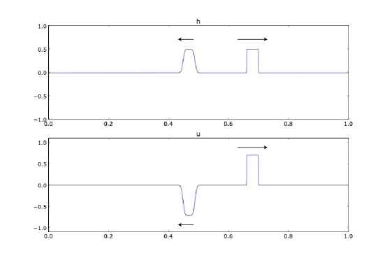
Figure 6: Snapshot of the solution of (25). The arrows point to the wave travel directions; longer arrows indicate greater speeds, but not proportionally.

We experiment with Type 1 and Type 2 mesh refinement strategies and compare the results with that of the uniform mesh refinement strategy. All strategies are applied with the same tolerance goal

$$TOL=4.0\times 10^{-4}$$

for the error. The uniform mesh refinement strategy requires 2,560 cells to reach the tolerance goal. The Type 1 strategy, i.e., time-unvarying adaptive mesh refinement, requires 1,200 cells to reach the same tolerance goal. The final grid is plotted in Fig. 7. We see that the grid is intensely refined over the travel ranges of both of the wave packets. The savings in number of cells come from the “quiet” regions where there are no wave activities. The refined region is shifted towards the right end because the rightward wave is traveling at a greater speed and thus has a longer travel range. We then apply the Type 2 strategy with three temporal sub-intervals over the whole simulation period $[0,T]$. The resulting grid that meets the tolerance is given in Fig. 8 and has 949 cells for the first sub-interval, 1143 for the second, and 179 for the last, with an average of 757 cells for the whole simulation period. The saving in the number of cells stems from the fact that when the wave packets are far apart, the surrounding regions for them can be refined separately and thus the unnecessary refinement in the middle is avoided.

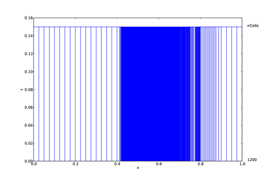
Figure 7: The final grid generated by the Type 1 adaptive mesh refinement strategy.

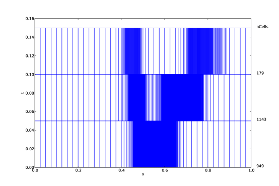
Figure 8: The final grid generated by the Type 2 adaptive mesh refinement strategy

4 Concluding remarks

In this article, we present a framework for goal-oriented a posteriori error estimation for finite volume methods. The formulation of the a posteriori error estimate is independent of the exact form of the methods and therefore can be applied to arbitrary finite volume methods. In this framework, it is not required that the adjoint equations be solved in a function space larger than that for the forward equation, due to the fact that finite volume methods, generally speaking, are not built on Galerkin orthogonality.

To demonstrate the validity of the a posteriori error estimate, we conduct numerical experiments with the one-dimensional linear transport equation. The primal equation is solved using the first-order, upwind finite volume method. The overall conclusion from these experiments is that the more accurate the adjoint solution is, the more accurate the a posteriori error estimate is. Roughly speaking, there are two scenarios one has to deal with in practice. If the quantity of interest is defined by a simple kernel function, then solving the adjoint equation with a numerical method of the same order or accuracy and with a mesh with resolution similar as that for the primal equation may prove adequate. If the quantity of interest is more complex, then the adjoint equation may have to be solved on a finer mesh or to be solved by a high-order accurate method. We have found that the latter approach is often more efficient.

An application of the a posteriori error estimate to adaptive mesh refinement is also presented. The one-dimensional linearized shallow-water equations are taken as an example. The test case involves two wave packets traveling in opposite directions with different speeds. This case is numerically very challenging. The a posteriori error estimate is found to be effective at guiding various adaptive mesh refinement strategies that lead to grids that are dynamically refined according to wave activities.

We can identify several directions or future work. The impact of the lack of accuracy in the adjoint solution on the accuracy of the a posteriori error estimate is only experimentally explored in this work. More rigorous analysis is warranted for this issue. A related issue is the impact of the substitution of the primal solution $\boldsymbol{u}$ by its approximation $\boldsymbol{u}^{\#}$ in the kernel function $\phi$. We did not touch upon this issue here, but it is very important and inevitable in cases involving nonlinear quantities of interest.

Another direction future research is to apply the framework of a posteriori error estimation, laid out in this article, to regional climate modeling, which is the primary motivation for the current work. An emerging approach towards climate modeling is to use one global grid over the whole sphere, with local refinements over regions of interest, and with smooth transitions between coarse and fine regions ([16]). In our opinion, the current mesh refinement strategy used in this approach is quite rudimentary in that it only refines over regions that are directly of interest. Goal-oriented error estimation is clearly needed to guide a more sensible mesh refinement strategy, and thus to control the computational errors with regard to the quantities of interest.

References

- [1] Y. Achdou, C. Bernardi, and F. Coquel, A priori and a posteriori analysis of finite volume discretizations of Darcy’s equations, Numer. Math. 96 (2003), no. 1, 17–42. MR 2018789 (2005d:65179)
- [2] M. Afif, A. Bergam, Z. Mghazli, and R. Verfürth, A posteriori estimators for the finite volume discretization of an elliptic problem, Numer. Algorithms 34 (2003), no. 2-4, 127–136, International Conference on Numerical Algorithms, Vol. II (Marrakesh, 2001). MR 2043890
- [3] Abdellatif Agouzal and Fabienne Oudin, A posteriori error estimator for finite volume methods, Appl. Math. Comput. 110 (2000), no. 2-3, 239–250. MR 1745373 (2001a:65134)
- [4] Timothy J. Barth and Mats G. Larson, A posteriori error estimates for higher order Godunov finite volume methods on unstructured meshes, Finite volumes for complex applications, III (Porquerolles, 2002), Hermes Sci. Publ., Paris, 2002, pp. 27–49. MR 2007403 (2004j:65132)
- [5] C. Carstensen, R. Lazarov, and S. Tomov, Explicit and averaging a posteriori error estimates for adaptive finite volume methods, SIAM J. Numer. Anal. 42 (2005), no. 6, 2496–2521 (electronic). MR 2139403 (2006b:65165)
- [6] Q. Chen, J. Laminie, A. Rousseau, R. Temam, and J. Tribbia, A 2.5D model for the equations of the ocean and the atmosphere, Anal. Appl. (Singap.) 5 (2007), no. 3, 199–229. MR MR2340646 (2008h:35281)
- [7] Qingshan Chen, Max Gunzburger, and Todd Ringler, A scale-invariant formulation of the anticipated potential vorticity method, Montly Weather Review, submitted.
- [8] Kenneth Eriksson, Don Estep, Peter Hansbo, and Claes Johnson, Introduction to adaptive methods for differential equations, Acta numerica, 1995, Acta Numer., Cambridge Univ. Press, Cambridge, 1995, pp. 105–158.
- [9] Don Estep, Michael Pernice, Du Pham, Simon Tavener, and Haiying Wang, A posteriori error analysis of a cell-centered finite volume method for semilinear elliptic problems, J. Comput. Appl. Math. 233 (2009), no. 2, 459–472. MR 2568539 (2010j:65214)
- [10] Lawrence C. Evans, Partial differential equations, second ed., Graduate Studies in Mathematics, vol. 19, American Mathematical Society, Providence, RI, 2010. MR 2597943
- [11] Jonathan E. Guyer, Daniel Wheeler, and James A. Warren, FiPy: Partial differential equations with Python, Computing in Science and Engineering 11 (2009), no. 3, 6–15.
- [12] Serge Nicaise, A posteriori error estimations of some cell-centered finite volume methods, SIAM J. Numer. Anal. 43 (2005), no. 4, 1481–1503 (electronic). MR 2182137 (2006j:65316)
- [13] , A posteriori error estimations of some cell centered finite volume methods for diffusion-convection-reaction problems, SIAM J. Numer. Anal. 44 (2006), no. 3, 949–978 (electronic). MR 2231851 (2007e:65124)
- [14] A. Pazy, Semigroups of linear operators and applications to partial differential equations, Applied Mathematical Sciences, vol. 44, Springer-Verlag, New York, 1983. MR 710486 (85g:47061)
- [15] T. D. Ringler, J. Thuburn, J. B. Klemp, and W. C. Skamarock, A unified approach to energy conservation and potential vorticity dynamics for arbitrarily-structured c-grids, J. Comput. Phys. 229 (2010), no. 9, 3065–3090.
- [16] Todd D. Ringler, Doug Jacobsen, Max Gunzburger, Lili Ju, Michael Duda, and William Skamarock, Exploring a multi-resolution modeling approach within the shallow-water equations, in preparation.
- [17] W. Rudin, Functional analysis, second ed., International Series in Pure and Applied Mathematics, McGraw-Hill Inc., New York, 1991. MR MR1157815 (92k:46001)
- [18] Martin Vohralík, Residual flux-based a posteriori error estimates for finite volume and related locally conservative methods, Numer. Math. 111 (2008), no. 1, 121–158. MR 2448206 (2009h:76142)
- [19] , Two types of guaranteed (and robust) a posteriori estimates for finite volume methods, Finite volumes for complex applications V, ISTE, London, 2008, pp. 649–656. MR 2451464