Optimization of artificial flockings by means of anisotropy measurements

Abstract

An effective procedure to determine the optimal parameters appearing in artificial flockings is proposed in terms of optimization problems. We numerically examine genetic algorithms (GAs) to determine the optimal set of parameters such as the weights for three essential interactions in BOIDS by Reynolds (1987) under ‘zero-collision’ and ‘no-breaking-up’ constraints. As a fitness function (the energy function) to be maximized by the GA, we choose the so-called the $\gamma$-value of anisotropy which can be observed empirically in typical flocks of starling. We confirm that the GA successfully finds the solution having a large $\gamma$-value leading-up to a strong anisotropy. The numerical experience shows that the procedure might enable us to make more realistic and efficient artificial flocking of starling even in our personal computers. We also evaluate two distinct types of interactions in agents, namely, metric and topological definitions of interactions. We confirmed that the topological definition can explain the empirical evidence much better than the metric definition does.

1 Introduction

Collective behaviour of interacting agents such as flying birds, moving insects or swimming fishes shows highly non-trivial properties. We sometimes find a kind of ‘beauty’ in the quite counter-intuitive and fascinating phenomena [1, 2, 3]. If one wishes to deal with these ingredients by mathematically rigorous approach, we sometimes regard each of them as a simple ‘particle’ without size and any specific shape. As a typical example of such ‘massive’ interacting particle systems, a critical phenomenon of order-disorder phase transitions with ‘spontaneous symmetry breaking’ in spatial structures of the so-called ferromagnetic Ising system has attracted much attention of physicists. Up to now, a huge number of numerical and analytical studies in order to figure it out have been done by theoretical physicists and mathematicians [4].

On the other hand, for the mathematical modelling of many-particle systems having interacting intelligent agents (animals), we also use some probabilistic models. For instance, in the research field of physics, Vicsek et.al. [5] proposed a flocking dynamics having a simple rule, namely, a given particle (agent) driven with a constant absolute velocity at each time step assumes the average direction of motion of the particles (agents) in its neighbourhood of radius $r$ with some random perturbation added.

In engineering, a simplest and effective algorithm called BOIDS [6, 7] has been widely used not only in the field of computer graphics but also in various other research fields including ethology, control theory and so on. The BOIDS simulates the collective behaviour of animal flocks by taking into account only a few simple rules for each interacting intelligent agent.

Recently, quite a lot of useful flocking algorithms inspired by the BOIDS were proposed by a combination of a velocity cooperation with a local potential-driven field (for instance, see [8, 9]). Among these studies, Olfati-Saber [10] provided a remarkable framework for designing of scalable flocking algorithms. His framework has three essential factors in the algorithm. The first one is the same three essential rules as those in the BOIDS we mentioned just above. The second factor is the ability of avoidance of unexpected obstacles appearing on the path of flock’s movement. The third and the most remarkable one is the ability for causing the flock to track the path of a single virtual leader by introducing a navigational feedback forth to each agent, namely, all agents in the flock are moving according to the information about the virtual leader. However, up to now, nobody knows whether such a virtual leader actually exists in real flocks or not.

Hence, it is very hard task for us to evaluate these modelings and also very difficult to judge whether it behaves like realistic or not due to a lack of enough empirical findings to be compared [11, 12, 13].

As we know from the above issue (doubt) as an example, one of the serious problems in studies of any artificial flocking (algorithm) is apparently a lack of empirical data to check the validity. Actually, there are few studies to compare the results of the flocking simulations with the empirical data. Therefore, the following essential queries still have been left unsolved;

• What is a criterion to determine to what extent the flocks seem to be realistic?

• Is there any quantity (statistics) to measure the quality of the artificial flocks?

• Is it possible for us to construct the mathematically defined ‘optimal’ BOIDS in computers? If possible, how does one design the optimal BOIDS in terms of some maximization (or minimization) principle of appropriate fitness functions?

From the view point of ‘engineering’, the above first two queries are somewhat not essential because their main goal is to build-up a useful algorithm based on the collective behaviour of agents. However, from the natural science view points, the difference between empirical evidence and the result of the simulation is the most important issue and the consistency is a guide to judge the validity of the computer modelling and simulation. On the other hand, the third query is very important for engineering to solve important problems in the real world by using the knowledge of such outstanding abilities of these intelligent flockings.

Recently, Ballerini et. al. [14] succeeded in obtaining the data for such collective animal behaviour, namely, empirical data of starling flocks containing up to a few thousands members. They also pointed out that the angular density of the nearest neighbours in the flocks is not uniform but apparently biased (it is weaken) along the direction of the flock’s motion.

With their empirical data by hand, in the previous paper [16], we examined the possibility of the BOIDS simulations to reproduce this anisotropy and we also investigated numerically the condition on which the anisotropy emerges.

However, in our previous studies, we checked only the existence of the anisotropy and did not check extensively the strength of the anisotropy which is measured by the $\gamma$-value. To make the matter worse, due to some technical limitations of computer simulations, we could not evaluate the $n$-th order nearest neighbouring dependence of the $\gamma$-value precisely. Namely, due to the following three bottlenecks, we could not check the validity of the BOIDS simulations by means of the anisotropy measurements:

• Bottleneck 1 : It is very hard to check whether the result comes from the nature of mathematical modelling or from the choice of parameters appearing in the model.

• Bottleneck 2 : It is very difficult for us to generate aggregations with a high $\gamma$-value which have been observed in a lot of empirical findings.

• Bottleneck 3 : It is very difficult to evaluate the $\gamma$-value precisely for the $n$-th order nearest neighbour due to the so-called border bias.

In this paper, in order to overcome the above Bottleneck 1 and Bottleneck 2, we propose and examine a genetic algorithm (GA) to maximize the $\gamma$-value which is implicitly regarded as a fitness function of the weights of essential three interactions, namely, Cohesion, Alignment and Separation, appearing in the BOIDS algorithm. By finding the optimal weights for the BOIDS, we expect that the $\gamma$-value for the ‘optimal’ BOIDS is enhanced by the appropriate choice of the weights. For the Bottleneck 3, we propose a border-bias free procedure to evaluate the $\gamma$-value in the computer simulations.

This paper is organized as follows. In the next section 2, we explain the concept of anisotropy measurement. The anisotropy distribution map and the measurement through the $\gamma$-value are also explained. In the next section 3, we explain the essential three interactions in the BOIDS. In section 4 and 5, we provide the set-up of scale-lengths and time-scale in our computer simulations. In section 6, we show the result without optimization as a preliminary. In the next section 7, we mention that the selecting the interactions in the BOIDS is formulated as an optimization problem to maximize the $\gamma$-value as the cost function. In section 8, we explain the genetic algorithm to maximize the cost function and why we use the algorithm. The results are shown in the next section 9. In these modelling, we assume that each agent interacts with the other mates within a fixed range of the visual field. In this sense, the model should be referred to as metric model. On the other hand, one can consider the topological model in which each agent interacts with a fixed number of the mates. In section 10, we apply our procedure to design the optimal BOIDS for the topological model and compare the result with that of the metric model. We find that the topological model can reproduce the empirical finding much better than the metric model does. In section 11, we discuss the results and the last section is summary.

2 Anisotropy in real and artificial flockings

In this section, we explain the concept of anisotropy in flockings originally proposed by Ballerini et. al. [14] to evaluate the empirical data of starling flockings. For the emergence of the anisotropy, we evaluate the strength of the anisotropy by the measurement, that is, the $\gamma$-value.

2.1 Emergence of anisotropy

Ballerini et. al. [14] measured each bird’s position in the flocks of starling (Sturnus vulgaris) for $8$ seconds in three dimension. To get such three dimensional data, they used ‘Stereo Matching’ which reconstructs three dimensional object from a set of stereo photographs. From these data, they calculated the angle between the direction of nearest neighbours and the direction of the flock’s motion for all birds in the flock. They measured the angles ($\phi$, $\alpha$), where $\phi$ means the latitude ($\in[-90^{\circ},90^{\circ}]$) of nearest neighbour for each bird measured from the direction of the flock’s motion, whereas the vertical axis $\alpha$ denotes longitude ($\in[-180^{\circ},180^{\circ}]$) which specifies the position of the nearest neighbour for each bird around the flock’s motion, of the nearest neighbour for all birds in the flock, and plot these angles in the two-dimensional map using the so-called Mollweide projection. To put it briefly, this map means the density of angular distribution of the nearest neighbour. Inspired by their empirical findings, we simulate the distribution map by BOIDS simulation [16]. The resultant angular distribution map is shown in Fig. 1. This figure clearly shows that the density is not uniform but obviously biased.

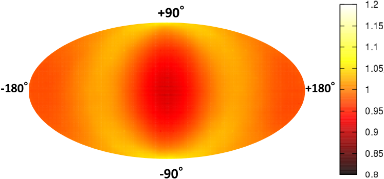
Figure 1: Angular distribution map simulated by BOIDS-based modelling (from Makiguchi and Inoue (2010) [16]).

2.2 Anisotropy measurement: Formula and generic properties

To evaluate the strength of the anisotropy, we use the $\gamma$-value which is an anisotropy measurement introduced by Ballerini et. al. [14]. In following, we briefly explain how to compute it and mention the general properties.

As a matter of convenience, let us first define the vector:

$$\mbox{\boldmath$u$}_{i}^{(n)}\equiv|u_{i}^{(n)}\rangle,\,\,\,((\mbox{\boldmath$u$}_{i}^{(n)})^{t}=(u_{ix}^{(n)},u_{iy}^{(n)},u_{iz}^{(n)})\equiv\langle u_{i}^{(n)}|)$$ (1)

in the Dirac’s bracket representation in quantum mechanics [17] as a three-dimensional unit vector pointing to the $n$-th nearest neighbouring agent (bird) from an arbitrary argent $i$.

We should keep in mind that $t$ appearing in the shoulder of matrix here such as $\mbox{\boldmath$A$}^{t}$ stands for the ‘transpose’. Then, we have the following $3\times 3$ projection matrix $\mbox{\boldmath$M$}^{(n)}$ in terms of the Dirac’s bracket:

$$\mbox{\boldmath$M$}^{(n)} = \frac{1}{N}\sum_{i=1}^{N}(|u_{i}^{(n)}\rangle\langle u_{i}^{(n)}|)$$ (2)

whose components are given by

$$(\mbox{\boldmath$M$}^{(n)})_{\alpha\beta} = \frac{1}{N}\sum_{i=1}^{N}(|u_{i}^{(n)}\rangle)_{\alpha}(|u_{i}^{(n)}\rangle)_{\beta}$$ (3)

for $\alpha,\beta=x,y,z$, where $N$ stands for the total number of agents in the flock. For the above $\mbox{\boldmath$M$}^{(n)}$, we immediately obtain the normalized eigenvectors $|U_{k}^{(n)}\rangle,k=1,2,3$, and one can rewrite the matrix $\mbox{\boldmath$M$}^{(n)}$ in terms of these bases as

$$\mbox{\boldmath$M$}^{(n)} = \sum_{k=1}^{3}\lambda_{k}|U_{k}^{(n)}\rangle\langle U_{k}^{(n)}|$$ (4)

where $\lambda_{k},k=1,2,3$ stand for the eigenvalues of the matrix, that is, $\mbox{\boldmath$M$}^{(n)}|U_{k}^{(n)}\rangle=\lambda_{k}|U_{k}^{(n)}\rangle,k=1,2,3$, and of course, the rectangular condition $\langle U_{k}^{(n)}|U_{l}^{(l)}\rangle=\delta_{k,l}$ is satisfied. It should be noted that when the projection matrix $\mbox{\boldmath$M$}^{(n)}$ becomes irregular, we cancel the observation in our calculations of the $\gamma$-value. Therefore, the probability $P_{k}$ that an arbitrary agent exists in the direction of the vector $|U_{k}^{(n)}\rangle$ is explicitly given by

$$P_{k} = |\langle U_{k}^{(n)}|\mbox{\boldmath$M$}^{(n)}|U_{k}^{(n)}\rangle|^{2}=\lambda_{k}^{2},\,\,\,k=1,2,3.$$ (5)

When we put these eigenvalues in a particular order, say, $\lambda_{1}<\lambda_{2}<\lambda_{3}$ (this reads $P_{1}<P_{2}<P_{3}$), the vector $|U_{3}^{(n)}\rangle$ is the direction in which the agents are more likely to exist, whereas there are fewest agents in the direction of vector $|U_{1}^{(n)}\rangle$. Therefore, if we define the emergence of anisotropy as the absence of the birds along the direction of the flock’ s motion, the strength of the anisotropy is naturally measured by the inner-product of the vector pointing to the flock’s movement and the eigenvector having the lowest eigenvalue.

To evaluate the anisotropy measurement more explicitly, let us define the eigenvector of the lowest eigenstate by $|W^{(n)}\rangle$, that is, $\langle W^{(n)}|\mbox{\boldmath$M$}^{(n)}|W^{(n)}\rangle=\min_{k}\lambda_{k}$. Then, the anisotropic measurement is calculated from the $|W^{(n)}\rangle$ and the vector $|V\rangle$ that points to the direction of the flock’s movement (the velocity of the center of mass in the flocking $|V\rangle\equiv(1/N)\sum_{i=1}^{N}\mbox{\boldmath$V$}_{i}$) as

$$\gamma_{t} = |\langle W^{(n)}|V\rangle|^{2}.$$ (6)

Obviously, the above $\gamma_{t}$ is dependent on the time $t$ through the time-dependence of $|V\rangle$ and $|W^{(n)}\rangle$. Thus, we define the anisotropic measurement $\gamma$ by averaging over the ‘observation-time’ with the infinite length $T\to\infty$ as

$$\gamma = \mathbb{E}_{t}[\gamma_{t}]\equiv\lim_{T\to\infty}\frac{1}{T}\sum_{t=1}^{T}\gamma_{t}.$$ (7)

As it is impossible to take the infinite observation-time limit $T\to\infty$ in computer, we replace the limit by finite observation-time, say, $T=80$ for the upper bound in the sum (7).

We should also keep in mind that the $\gamma$-value depends on the choice of initial conditions and one should take the average over the distribution of initial conditions. However, we might expect that the $\gamma$-value calculated for a single realization of initial conditions, say, $\gamma$ is identical to its average $\mathbb{E}_{ini.}[\cdots]$ over the initial condition, namely, $\gamma=\mathbb{E}_{ini.}[\gamma]$ in the limit of $N\to\infty$. As we shall show later, the number of agents in our simulation is too small $N=100\ll\infty$ to satisfy the above condition. Therefore, we calculate the average of the $\gamma$-value for $1000$-independent initial conditions.

It should be noted that the $\gamma$-value takes any positive values in the range $0\leq\gamma\leq 1$. For the case of $\gamma=0$, the nearest neighbour is more likely to exist in the direction of flock’s movement, namely, $\langle W^{(n)}|V\rangle=0$. On the other hand, the $\gamma=1$ implies that the nearest neighbour exist in the two-dimensional plane which is perpendicular to the flock’s movement with probability $1$, that is to say, $|W^{(n)}\rangle=\pm|V\rangle$ resulting in $|\langle W^{(n)}|V\rangle|^{2}=1$. We should notice that for the eigenvector $|S^{(n)}\rangle$ and $|S_{2}^{(n)}\rangle$ having the largest and the second largest eigenvalues, $|\langle S^{(n)}|V\rangle|^{2}+|\langle S_{2}^{(n)}|V\rangle|^{2}=1$ for $\gamma=0$ and $\langle S^{(n)}|V\rangle=\langle S_{2}^{(n)}|V\rangle=0$ for $\gamma=1$ should be satisfied.

After simple algebra, one can show that the $\gamma$ takes $1/3$ when there is no spatial bias in the direction of the nearest neighbours (namely isotropy). This means that the anisotropy emerges when the following condition is satisfied.

$$\gamma > \gamma_{\rm uniform}\equiv\frac{1}{3}$$ (8)

In fact, the above inequality is easily confirmed. The $\gamma$-value for the uniform distribution of the position $(\phi,\alpha)$, where $\phi$ and $\alpha$ are the same variables of angles defined in the previous subsection, for a given vector $|V\rangle$, namely, the $\gamma$-value for $\rho(\phi,\alpha)=(4\pi)^{-1}$ is easily calculated as

$$\gamma_{\rm uniform} = \int_{\rm sphere}\rho(\phi,\alpha)\,d\phi\,d\alpha|\langle W^{(n)}|V\rangle|^{2}=\frac{1}{4\pi}\int_{-\pi}^{\pi}\cos^{2}\alpha\,d\alpha\int_{-\frac{\pi}{2}}^{\frac{\pi}{2}}\cos^{3}\phi\,d\phi$$ (9)

$$= \frac{1}{3}$$

where we used $|\langle W^{(n)}|V\rangle|^{2}=\cos^{2}\phi\cos^{2}\alpha$. Therefore, the distribution of the $n$-th nearest neighbours has an anisotropic structure when the $\gamma$-value is larger than $\gamma_{\rm uniform}=1/3$, namely the condition for the emergence of the anisotropy is explicitly written by (8).

Ballerini et. al. [14] measured the $\gamma$-value up to the $n$-th order of nearest neighbours for two kinds of empirical data having different numbers of agents and show the $n$-dependence of the $\gamma$-value. From their plot, we clearly find that $\gamma$-value takes larger than $0.8$ for $n=1$ and the value remains larger than $\gamma_{\rm uniform}=1/3$ up to $n=6$. In our previous studies [16], the $n$-dependence of the $\gamma$-value was evaluated for the data generated artificially from BOIDS simulations, however, we could not overcome the problem of border bias which was mentioned as Bottleneck 3 in the previous section. In this paper, we introduce a way to overcome this technical difficulty and attempt to measure the $\gamma$-value more precisely.

3 Essential three interactions in BOIDS

To make flock simulations in computer, we use the so-called BOIDS which was originally designed by Reynolds in 1987 [6]. The BOIDS is one of the well-known mathematical (probabilistic) models in the research fields of CG and animation. Actually, the BOIDS can simulate very complicated animal flocks or schools although it consists of just only three simple interactions for each agent in the aggregation:

1. Cohesion: Making each agent’s position $\mbox{\boldmath$X$}_{i}\,(i=1,\cdots,N)$ toward the average position of neighbouring flock mates.

2. Alignment: Keeping the velocity of each agent $\mbox{\boldmath$V$}_{i}\,(i=1,\cdots,N)$ the average value of neighbouring flock mates.

3. Separation: Making a vector of each agent’s position $\mbox{\boldmath$X$}_{i}\,(i=1,\cdots,N)$ to avoid the collision with the neighbouring flock mates.

Each agent decides her (or his) next direction of migration by compounding these three vectors of interaction. In addition to this, it is important for us to bear in mind that ‘local flock mates’ mentioned above denotes the neighbours within the range of view for each agent. We explain this view and other settings of our simulation in the next section.

3.1 BOIDS dynamics

For simplicity, we define ‘neighbouring mates’ by all metes which exist within the visual field with a radius $R$ and for each mate categorized as the neighbouring mates, we calculate the interactions of Cohesion and Alignment as normalized unit vectors. In addition, we evaluate the interaction of Separation as a unit vector pointing to the direction of fading-out from the mates. Each agent $i$ updates its own velocity vector $\mbox{\boldmath$V$}_{i}$ and the position $\mbox{\boldmath$X$}_{i}$ by the following recursion relations.

$$\mbox{\boldmath$V$}_{i}(l+1) = \overline{V}_{l}^{(i)}\mbox{\boldmath$e$}_{B}^{(i)}(l)$$ (10)

$$\mbox{\boldmath$X$}_{i}(l+1) = \mbox{\boldmath$X$}_{i}(l)+\mbox{\boldmath$V$}_{i}(l+1)$$ (11)

where $l$ denotes time step in our simulations and we discretized the infinitesimal time as a unit time step $\Delta l=l+1-l=1$ in the definition of velocity $\mbox{\boldmath$V$}_{i}=d\mbox{\boldmath$X$}_{i}/dl\simeq\{\mbox{\boldmath$X$}_{i}(l+\Delta l)-\mbox{\boldmath$X$}_{i}(l)\}/\Delta l=\mbox{\boldmath$X$}_{i}(l+1)-\mbox{\boldmath$X$}_{i}(l)\equiv\mbox{\boldmath$V$}_{i}(l+1)$ to obtain (11). $\mbox{\boldmath$e$}_{B}^{(i)}(l)$ denotes a unit vector pointing to the direction to which the agent $i$ should move according to the BOIDS. The $\mbox{\boldmath$e$}_{B}^{(i)}(l)$ is explicitly given by

$$\mbox{\boldmath$e$}_{B}^{(i)}(l) = \frac{\frac{J_{1}\mbox{\boldmath$v$}_{\rm C}^{(i)}(l)+J_{2}\mbox{\boldmath$v$}_{\rm A}^{(i)}(l)+J_{3}\mbox{\boldmath$v$}_{\rm S}^{(i)}(l)}{|J_{1}\mbox{\boldmath$v$}_{\rm C}^{(i)}(l)+J_{2}\mbox{\boldmath$v$}_{\rm A}^{(i)}(l)+J_{3}\mbox{\boldmath$v$}_{\rm S}^{(i)}(l)|}+\eta\frac{\mbox{\boldmath$V$}_{i}(l)}{|\mbox{\boldmath$V$}_{i}(l)|}}{\left|\frac{J_{1}\mbox{\boldmath$v$}_{\rm C}^{(i)}(l)+J_{2}\mbox{\boldmath$v$}_{\rm A}^{(i)}(l)+J_{3}\mbox{\boldmath$v$}_{\rm S}^{(i)}(l)}{|J_{1}\mbox{\boldmath$v$}_{\rm C}^{(i)}(l)+J_{2}\mbox{\boldmath$v$}_{\rm A}^{(i)}(l)+J_{3}\mbox{\boldmath$v$}_{\rm S}^{(i)}(l)|}+\eta\frac{\mbox{\boldmath$V$}_{i}(l)}{|\mbox{\boldmath$V$}_{i}(l)|}\right|}$$ (12)

with

$$\mbox{\boldmath$v$}_{\rm C}^{(i)}(l) = \frac{\frac{\sum_{j=1}^{N}\Theta(R-r_{ij})\mbox{\boldmath$X$}_{j}(l)}{\sum_{j=1}^{N}\Theta(R-r_{ij})}-\mbox{\boldmath$X$}_{i}(l)}{\left|\frac{\sum_{j=1}^{N}\Theta(R-r_{ij})\mbox{\boldmath$X$}_{j}(l)}{\sum_{j=1}^{N}\Theta(R-r_{ij})}-\mbox{\boldmath$X$}_{i}(l)\right|}$$ (13)

$$\mbox{\boldmath$v$}_{\rm A}^{(i)}(l) = \frac{\sum_{j=1}^{N}\Theta(R-r_{ij})\mbox{\boldmath$V$}_{j}(l)}{|\sum_{j=1}^{N}\Theta(R-r_{ij})\mbox{\boldmath$V$}_{j}(l)|}$$ (14)

$$\mbox{\boldmath$v$}_{\rm S}^{(i)}(l) = -\frac{\sum_{j=1}^{N}\Theta(R-r_{ij})(\mbox{\boldmath$X$}_{j}(l)-\mbox{\boldmath$X$}_{i}(l))}{|\sum_{j=1}^{N}\Theta(R-r_{ij})(\mbox{\boldmath$X$}_{j}(l)-\mbox{\boldmath$X$}_{i}(l))|}$$ (15)

where we defined $r_{ij}$ as the square distance between agent $i$ and $j$ as

$$r_{ij} \equiv |\mbox{\boldmath$X$}_{i}(l)-\mbox{\boldmath$X$}_{j}(l)|=\sqrt{\{\mbox{\boldmath$X$}_{i}(l)-\mbox{\boldmath$X$}_{j}(l)\}^{2}}.$$ (16)

$\Theta(\cdots)$ denotes a step function. Therefore, $\sum_{j=1}^{N}\Theta(R-r_{ij})$ stands for the number of ‘neighbouring mates’ for the agent $i$ and the number is obviously dependent on the agent $i$.

A balance parameter $\eta$ appearing in (12) determines the weights of two distinct modifications $\mbox{\boldmath$e$}_{B}^{(i)}(l)$ for the velocity vector for the agent $i$, namely, the ‘BOIDS-driven’ correction term $\sim\,J_{1}\mbox{\boldmath$v$}_{\rm C}^{(i)}(l)+J_{2}\mbox{\boldmath$v$}_{\rm A}^{(i)}(l)+J_{3}\mbox{\boldmath$v$}_{\rm S}^{(i)}(l)$ and the vector conservation term $\sim\,\mbox{\boldmath$V$}_{i}(l)$. Hence, the vector $\mbox{\boldmath$V$}_{i}(l)$ is conserved for $\eta\gg 1$, whereas the dynamics of $\mbox{\boldmath$V$}_{i}(l)$ becomes purely BOIDS-driven for $\eta\ll 1$. Therefore, the choice of $\eta$ is regarded as a kind of ‘inert effect’ in the dynamics of BOIDS. The value itself should be determined empirically. However, due to the lack of such useful information about the inertia in real flockings, here we simply set $\eta=2$ by ad-hoc manner.

From the above definition of (13), we easily find that $\mbox{\boldmath$v$}_{\rm C}^{(i)}(l)=-\mbox{\boldmath$v$}_{\rm S}^{(i)}(l)$ and one of these two distinct effects is completely cancelled in the BOIDS dynamics (10)(11) as $\sim(J_{1}-J_{3})\mbox{\boldmath$v$}_{\rm C}^{(i)}(l)$ for any choice of $J_{1},J_{3}$. To correct this undesirable situation, we slightly modify the $\mbox{\boldmath$v$}_{\rm S}^{(i)}(l)$ as follows.

$$\mbox{\boldmath$v$}_{\rm S}^{(i)}(l) = -\frac{\Theta(R_{0}-r_{i\overline{j(1:i)}})(\mbox{\boldmath$X$}_{\overline{j(1:i)}}(l)-\mbox{\boldmath$X$}_{i}(l))}{|\Theta(R_{0}-r_{i\overline{j(1:i)}})(\mbox{\boldmath$X$}_{\overline{j(1:i)}}(l)-\mbox{\boldmath$X$}_{i}(l))|}$$ (17)

where $\overline{j(n:i)}$ denotes the $n$-th nearest neighbouring mate of the agent $i$ and it is explicitly given by :

$$\overline{j(n:i)} \equiv {\rm argmax}_{j\neq\overline{j(n-1:i)},\cdots,\overline{j(0:i)}}\,\,r_{ij}$$ (18)

with $\overline{j(0:i)}\equiv i$. Then, $\overline{j(1:i)}$ means the nearest neighbouring site

$$\overline{j(1:i)} \equiv {\rm arg}\min_{j}r_{ij}$$ (19)

for each $i$. Namely, the separation $\mbox{\boldmath$v$}_{\rm S}^{(i)}(l)$ acts if and only if the distance between the agent $i$ and the nearest neighbouring mate $\overline{j(1:i)}$ is lower than the radius of separation range $R_{0}$.

The vectors $\mbox{\boldmath$v$}_{\rm C}^{(i)}(l),\mbox{\boldmath$v$}_{\rm A}^{(i)}(l)$ and $\mbox{\boldmath$v$}_{\rm S}^{(i)}(l)$ denote the components caused by the interactions Cohesion, Alignment and Separation for agent $i$ at time $l$, respectively. We should keep in mind that $|\mbox{\boldmath$v$}_{\rm C}^{(i)}(l)|=|\mbox{\boldmath$v$}_{\rm A}^{(i)}(l)|=|\mbox{\boldmath$v$}_{\rm S}^{(i)}(l)|=1$ holds and $\mbox{\boldmath$J$}=(J_{1},J_{2},J_{3})$ stands for the set of weights for three interactions, namely, Cohesion, Alignment and Separation. We should keep in mind that from (13), (14) and (15), the weight $J_{2}$ is a ‘dimension-less’ variable, however, $J_{1}$ and $J_{3}$ have inverse-time dimension $\sim(\mbox{time step})^{-1}$.

We should keep in mind that the above definition of $\overline{j(n:i)}$, the $\gamma$-value is calculated by setting $|u_{i}^{(n)}\rangle\equiv\mbox{\boldmath$u$}_{i}^{(n)}=(\mbox{\boldmath$V$}_{i\overline{j(n:i)}}-\mbox{\boldmath$V$}_{i})/{|\mbox{\boldmath$V$}_{i\overline{j(n:i)}}-\mbox{\boldmath$V$}_{i}|}$ in (3)(6) and (7).

From equation (10), we are confirmed that the amplitude of velocity vector of agent $i$ at time $l+1$ is identical to the average amplitude of velocity vectors for neighbouring mates in the previous time step $l$ as

$$|\mbox{\boldmath$V$}_{i}(l+1)| = \overline{V}_{l}^{(i)}\equiv\frac{\sum_{j=1}^{N}\Theta(R-r_{ij})|\mbox{\boldmath$V$}_{j}(l)|}{\sum_{j=1}^{N}\Theta(R-r_{ij})}.$$ (20)

The above update rules (10), (11), (12), (13), (14) and (17) are our basic dynamical equations to be evaluated numerically.

Obviously, the behaviour of the artificial flockings strongly depends on the choice of the weights, however, there is no extensive study to investigate to what extent the behaviour changes quantitatively by changing the weights. From the fact in mind, in this paper, we propose a systematic algorithm to determine the weight by using the evolutionary computation such as GAs to maximize the $\gamma$-value as a fitness function.

4 Scale-lengths in BOIDS simulations

We here explain how we set several scale-lengths appearing in our simulations. In our previous studies, we determined them without any justification from the empirical evidence, however, here we attempt choose the scale lengths by taking into account the data from the reference [15] in order to realize the artificial flockings as realistic as possible (We summarize these variables in Table 1).

However, some parameters is not determined by empirical data, for instance, the range of interaction, the Frame-Rate (FR) [fps:frame-per-second] and so on. Therefor we set these parameter by the subjective view point and some regards for the calculation cost, for example, the number of agents $N=100$, the radius of the visual field $R=3\times R_{0}$ where $R_{0}=1.09$ [m] denotes the radius of separation range and the $FR$, which will be explained in the next section in detail, is $200$ [Hz].

A set of scale-lengths in our BOIDS
Number of agents ($N$)	100
Body-Length ($BL$)	0.2 [m]
Wing-Span ($WS$)	0.4 [m]
Radius of Separation Range ($R_{0}$)	1.09 [m]
Radius of Visual Field ($R$)	3 $\times$ $R_{0}$ [m]
Initial Speed Average ($V^{{}^{\prime}}$)	10.10 [m/s]
Initial Density of the Aggregation ($\rho$)	0.13 [${\rm m}^{-3}$]

Table 1: A set of scale-lengths in our flock simulation. Variables other than the Number of agents and the Radius of Visual Field are based on empirical data by Ballerini et. al. (Event 29-03 in Table 1 of [15]).

5 On the time-scale in BOIDS simulations

In our previous study [16], we defined the unit time (frame) by $0.1$ [sec]. In this paper, we shall define the frame based on the so-called Frame-Rate($FR=200$[Hz]). In order to consider the consistency with the empirical data analysis by Ballerini et. al. [14] in which they used $0.1$ [sec] for a unit frame, we evaluate the $\gamma$-value every $FR/20$ frames and the distance covered by each agent per frame, that is, the average of flock’s velocity $V$ is also determined from the empirical evidence of velocity $V^{{}^{\prime}}$ [m/sec] as $V=V^{{}^{\prime}}/FR$ [${\rm frame}^{-1}$].

In our previous work [16], we also chose the initial velocity for each agent from a uniform distribution having a finite support. However, this procedure might cause some difficulties, namely, we might encounter the ‘breaking-up’ of the flocking to several small groups due to synchronization in their speeds of convergence. In general, it is very difficult for us to control the speed of the flocking (the speed of the center of mass) after each agent’s speed converges when we determine the initial speed of each agent by a random number from a uniform distribution. To overcome this type of difficulties, we sample the initial value of each agent’s velocity $V_{i}$ from the following Gaussian with mean $V^{{}^{\prime}}=10.10$ [m/sec] and variance $\sigma^{2}=(V^{{}^{\prime}}-1)/3$, namely,

$$P(V_{i}) = \frac{1}{\sqrt{2\pi}\sigma}\,{\exp}\left[-\frac{(V_{i}-V^{{}^{\prime}})^{2}}{2\sigma^{2}}\right].$$ (21)

By this setting, we are confirmed that the speed of flocking actually converges to $V^{{}^{\prime}}$.

6 A preliminary: Simulations without GA

In this section, we show the results without any searching of the optimal weights of interactions by genetic algorithms as a preliminary.

6.1 Preliminary results

In the above setting of the problem, we attempt to evaluate the $\gamma$-value using the same way as our previous study [16]. We control the weights of three interactions in the BOIDS $\mbox{\boldmath$J$}=(J_{1},J_{2},J_{3})$ to generate typical three cases, namely, Crowded for $(J_{1},J_{2},J_{3})=(1,0,0)$, Synchronized for $(J_{1},J_{2},J_{3})=(0,1,0)$ and Spread for $(J_{1},J_{2},J_{3})=(0,0,1)$. We list the $\gamma$-values and the corresponding frequency of collisions (FC) in Table 2.

Behaviour	Weight vector $J$	$\gamma$-value [$SD$]	$FC$
Crowded	(1,0,0)	0.332 [0.0816]	100%
Synchronized	(0,1,0)	0.319 [0.292]	17.93%
Spread	(0,0,1)	0.347 [0.304]	0%

Table 2: Resulting $\gamma$-value and the SD (Standard Deviation), and the FC (Frequency of Collisions) are shown for three different ad-hoc choices of the weights $(J_{1},J_{2},J_{3})$.

We also show the angular distribution maps in Fig. 2. From these table and figure, we clearly find that in all cases, the anisotropy is not observed at all.

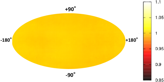
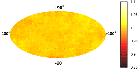
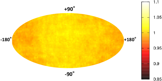
Figure 2: From the top to the bottom, the angular distribution maps for Crowded, Synchronized and Spread cases. In all cases, the anisotropy is not observed at all.

We next choose the weights $J_{1}$ and $J_{2}$ as $J_{1}=1,J_{2}=5$ which we used in the previous study [16] as an appropriate choice to produce the anisotropy, and we shall vary the $J_{3}$ from $0.2$ to $2.0$ to evaluate the $\gamma$-value and the corresponding frequency of collisions as a function of $J_{3}$. We plot them in Fig. 3.

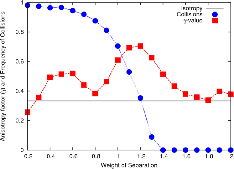
Figure 3: The $\gamma$-value and the corresponding frequency of collisions as a function of $J_{3}$ we set $J_{1}=1,J_{2}=5$. The frequency of collisions drops to zero around $J_{3}=1.4$. This fact makes us determine to choose the appropriate set as $(J_{1},J_{2},J_{3})=(1,5,1.4)$.

From this figure, we find that the frequency of collisions decreases monotonically as $J_{3}$ increases and it converges to zero around $J_{3}=1.4$. On the other hand, the $\gamma$-value takes its maximum $0.70$ around $J_{3}=1.2$. From these observations, we conclude that we should choose the weight as $\mbox{\boldmath$J$}=(J_{1},J_{2},J_{3})=(1,5,1.4)$ and whose $\gamma$-value will be about 0.70 .

7 Optimization to design artificial flockings

In the previous section, we show on what condition the anisotropy emerges by setting the weights for three essential interactions by ad-hoc manner as a preliminary. Here we mention that the procedure to determine the interactions can be regarded as a kind of optimization problems.

7.1 Optimization under two essential constraints

In real flockings, it might be a very serious problem for each agent how to refuse collisions with the other mates during the flock is moving. In addition, it is very hard for us to say that the flock splitting into several sub-flocks is also ‘realistic’ flocking. Therefore, we should design the BOIDS simulations so as to avoid these two unexpected accidents, namely, ‘collision’ and ‘breaking-up’. To realize the simulation in which there are no collision and breaking-up, we introduce two constrains into the optimization problem.

We first define the ‘collision’ as the case in which the distance between an arbitrary agent $i$ and its $1$-st nearest neighbouring mate $\overline{j(1:i)}$, say, $r_{i\overline{j(1:i)}}$ is shorter than their body length BL$=0.2$. We also assume that the ‘breaking-up’ occurs when the distance between the center of mass and the most far agent from it becomes longer than a given constant. It is naturally imagined that taking into account the ‘collision’ and making the algorithm to avoid it are essential issues not only for artificial flockings but also for flockings in the real world. It should be noted that the conventional flocking simulations based on the ‘particle models’ (see for example [10]) in which the size of the mate is neglected cannot deal with the ‘collision’. We are also confirmed that avoiding the ‘breaking-up’ also might be an essential factor to decide the size of the flocking.

Thus, we might use the $\gamma$-value as a cost function (energy function) to be minimized under ‘zero-collision’ and ‘zero-breaking-up’ constraint to determine the three essential interactions $\mbox{\boldmath$J$}=(J_{1},J_{2},J_{3})$. Namely, we should solve the following optimization problem with the cost.

$$E(\mbox{\boldmath$J$}) = \gamma(\mbox{\boldmath$J$})+\lambda_{1}\mathcal{N}(\mbox{\boldmath$J$})+\lambda_{2}\mathcal{B}(\mbox{\boldmath$J$}),\,\,\,\lambda_{1},\lambda_{2}\to\infty$$ (22)

where we defined $\mathcal{N}$ and $\mathcal{B}$ as the number of the collisions and breaking-up, respectively. The $\lambda_{1},\lambda_{2}$ stand for the Lagrange multipliers. In other words, the optimal interactions $\mbox{\boldmath$J$}_{\rm opt}$ is given by

$$\mbox{\boldmath$J$}_{\rm opt}={\rm argmax}_{\mbox{\boldmath$J$}}\lim_{\lambda_{1},\lambda_{2}\to\infty}E(\mbox{\boldmath$J$}).$$ (23)

Since Reynolds proposed the BOIDS, quite a lot of the modifications or the variants were constructed in terms of engineering, however, no studies concerning the systematic determination of the essential three interactions in the algorithm from the view point of empirical observation on real flockings such as starlings. Therefore, here we formulate the procedure to determine the interactions as optimization problems having the $\gamma$-value as the cost under two essential constraints. To solve the optimization problem by means of the conventional tools, say, genetic algorithm (GA for short), we might design the BOIDS more systematically. In the next section, we shall examine the GA to solve our optimization problem to determine the optimal set of the interactions in the BOIDS.

8 Genetic algorithms

Here we apply the GA to the determination of the weights of the interactions $J$ in BOIDS simulations. Before we show the results, we shall briefly explain the motivation to use the GA and the outline of the set-up and the procedure. The details of the GA shall be explained in Appendix A.

8.1 Why do we use the GA?

The GA is a stochastic method to obtain a candidate of the solution having the highest possible fitness in the complicated fitness function with multi-valley structures. In GAs, one codes the candidates of the solution by a set of vectors, each of which is referred to as a ‘gene configuration’ (a genetic code). Then, we make several operations, namely, Crossover, Mutation and Selection to regenerate gene configurations having relatively high fitness values [18].

As a study to determine the weights for the interactions in the BOIDS, Chen et. al. [19] proposed the so-called Interactive genetic algorithm (IGA). However, we should mention here that they used the fitness function which is constructed subjectively, and in this sense, their approach is essentially different from ours. This is because as we already mentioned, we use the $\gamma$-value which is a measurement introduced by empirical findings [14].

Of course, there are a lot of optimization methods and we do not have to use the GA to obtain the solution to maximize the $\gamma$-value. However, we might assume that the agent (bird for instance) acquired such an intelligent way to behave as ‘flock’ during their process of evolution and this assumption makes us use the GA. The justification of using the GA is very difficult to show and it might be impossible to prove the validity of the above assumption theoretically. Nevertheless, here we use the GA as a first attempt to design the optimal BOIDS based on the maximization principle of the $\gamma$-value as a fitness function.

8.2 Procedure of the GA

In this subsection, we shall explain the outline of the procedure of the GA. In our GA, we use the three weights of the BOIDS, namely, $\mbox{\boldmath$J$}=(J_{1},J_{2},J_{3})$ as gene configurations. Each of the components $J_{i}$ denotes a ‘chromosome’ or simply ‘gene’ and takes the value in the range $[0.001,0.999]$ and the minimum value of changing the state is set to $0.001$, namely, we here vary the value of each component by $J_{i}\to J_{i}\pm 0.001,\,\,i=1,2,3$ for each step of three operations we mentioned above.

To operate the Selection, we need the value of the fitness function, namely, the $\gamma$-value for the nearest neighbouring agent ($\gamma$-value defined by (7) with $n=1$). To evaluate it, we use the time-averaged $\gamma$-value $\mathbb{E}_{t}[\gamma_{t}]$ (see (7) for its definition) which is calculated by sampling positions of the mates every $0.1$ [sec] during $8$ [sec] ($T=80$ data points are needed to evaluate the $\gamma$-value for each update of the gene configurations). The details of the total procedure of the GA is given in Appendix A.

We also explain a border-bias free (the ‘border-bias’ was already mentioned in the section of introduction as Bottleneck 3) procedure to evaluate the $\gamma$-value in the computer simulations in Appendix B.

9 Results

In Table.3, We show the highest $\gamma$-values for three independent runs, which are referred to as Case 1,2 and Case 3, and corresponding weights for the interactions. It should be noted that we normalized the weights $\mbox{\boldmath$J$}=(J_{1},J_{2},J_{3})$ so as to make the maximum $J_{i}$ among the three $i=1,2,3$ unity.

Case	$\gamma$-value	$J_{1}$	$J_{2}$	$J_{3}$
Case 1	0.795	0.270	0.640	1
Case 2	0.797	0.234	0.699	1
Case 3	0.797	0.190	0.895	1

Table 3: Resultant sets of weights for three interactions.

For each run, the highest $\gamma$-value is larger than $0.79$ and corresponding weights $\mbox{\boldmath$J$}=(J_{1},J_{2},J_{3})$ take similar values for all cases. In following, we investigate the optimization process for Case 3.

9.1 Optimization process of GA

We show the minimum, average and maximum of the $\gamma$-value for each generation in Fig. 4. From this figure, we find that these all values converge to $\gamma\simeq 0.8$ from the initial state ($\gamma\simeq 0.4$).

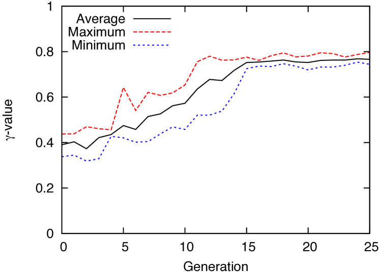
Figure 4: Evolution of $\gamma$-value in generations.

We next show the time evolution of the weights $\mbox{\boldmath$J$}=(J_{1},J_{2},J_{3})$ for the best possible gene configuration having the highest $\gamma$-value in Fig.5. From this figure, we find that each weight changes its state during the GA dynamics and this result tells us that optimal gene configuration can be successfully generated by our GA procedure.

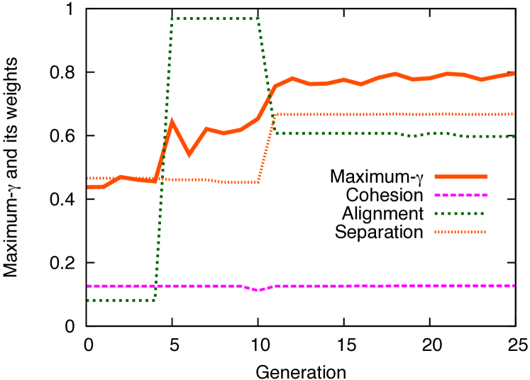
Figure 5: Evolutions of ‘Maximum-$\gamma$’ (the highest $\gamma$-value), $J_{1},J_{2}$ and $J_{3}$ in generations.

We also plot the distribution of $\gamma$-value at the initial generation (Fig.6 (left)) and at the final generation (Fig.6 (right)). From these two panels, we are confirmed that the gene configurations having relatively high fitness values are generated and they actually survive until the final generation. However, the final distribution has a finite deviation instead of a single delta peak. This means that we could not find the optimal gene configuration with probability $1$.

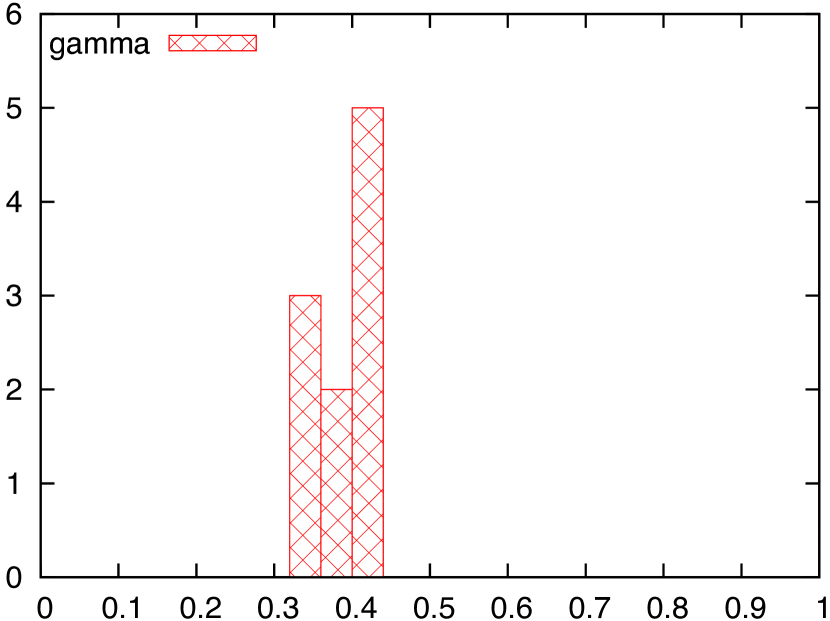
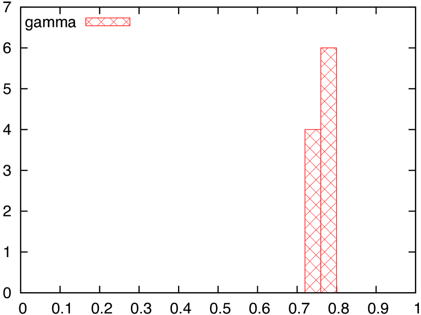
Figure 6: Left: Histogram of $\gamma$-value for the initial. Right: Histogram of $\gamma$-value for the final. We are confirmed that the GA successfully finds the value which is close to the highest possible $\gamma$-value with a high probability.

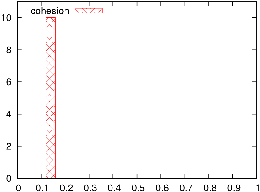
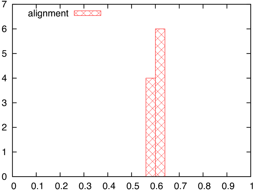
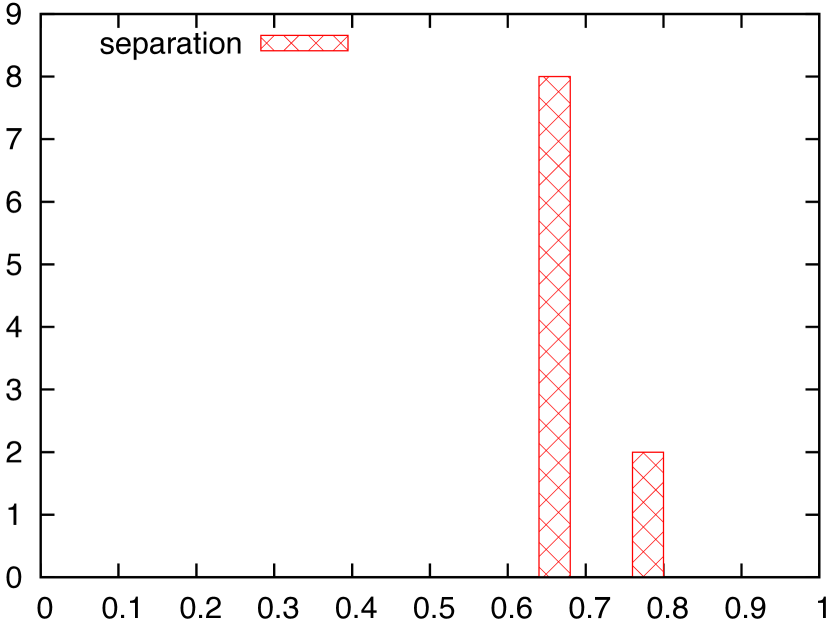
Figure 7: Histogram of weight of each interaction for the final gene set. Left: weight of ‘Cohesion’. Center: weight of ‘Alignment’. Right: weight of ‘Separation’.

9.2 The $\gamma$-value for the optimal BOIDS

Here we examine the $n$-th nearest neighbouring agent’s $\gamma$-value for the optimal BOIDS having the optimal weights obtained in the previous section. We carry out $1000$-trials to evaluate the $\gamma$-value for each $n$ from $n=1$ up to $n=25$. We also show the angular distribution map for $n=1$ and check the behaviour by graphical user interface (GUI). The results are shown in Fig.8.

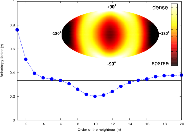
Figure 8: The $\gamma$-value as a function of $n$ calculated by the ‘optimal’ BOIDS simulation. The inset stands for the corresponding angular distribution.

From this figure, we find that the $\gamma$-value for $n=1$ takes the highest value which was also observed in the empirical data analysis [14]. We also find from the GUI that a realistic flocking’s behaviour in which the distance between nearest neighbouring agents is not zero (‘zero-collision’) but finite is achieved for the BOIDS with optimal weights of the interactions .

9.3 Anti-anisotropy effect and its possible explanation

In Fig.8, we find that the $\gamma$-value becomes lower than the isotropic limit $\gamma=1/3$ for $7\leq n\leq 14$. This ‘anti-anisotropy’ effect can be explained from the view point of geometric structure of the flocking as follows.

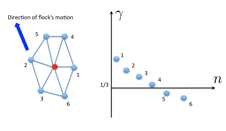
Figure 9: A reasonable explanation of the ‘anti-anisotropy’. The fifth and the sixth nearest neighbouring mates are more likely to exist in the direction of flock’s motion (left). As the result, the $\gamma$-values for the $5,6$-th orders of the nearest neighbouring become lower than the isotropic limit $1/3$ (right).

When we assume $2$-Dimensional Field and an arbitrary agent is surrounded by the other six mates as shown in Fig. 9 (this hexagon-shape is made by equilateral triangle with neighbours), the fifth and the sixth nearest neighbouring mates are more likely to exist in the direction of flock’s motion (they are indicated by ‘5’ and ‘6’ in Fig. 9 (left)). As the result, the $\gamma$-values for the $5,6$-th orders of the nearest neighbouring become lower than the isotropic limit $1/3$ (see Fig. 9 (right)). We should keep in mind that the ‘anti-anisotropy’ effect might appear much more clearly for the flocking being longer (in the moving direction) than is wide.

To confirm this assumption much more explicitly, we evaluate the third-power of average distance $R$ between an arbitrary agent and the $n$-th nearest neighbouring mate as a function of $n$.

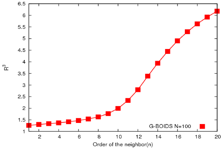
Figure 10: Third-power of average distance $R$ between an arbitrary agent and the $n$-th nearest neighbouring mate as a function of order of neighbour $n$. We are confirmed that the $R^{3}$ is almost constant up to the $8\sim 10$-th nearest neighbour.

We show the result in Fig. 10. From this figure, we clearly find that the $R^{3}$ is almost constant up to the $8\sim 10$-th nearest neighbour. This numerical result tells us that an arbitrary agent might be surrounded by $8\sim 10$ mates leading to the regular-polygon structure.

In the empirical data analysis of starling flocking, such ‘anti-anisotropy’ has never observed. Therefore, we might conclude that it is very hard for us to accept the regular-polygon structure around an arbitrary agent although our algorithm presented in this paper suggested the possibility (Appendix A).

10 Topological definition of neighbours in BOIDS

In the previous sections, we attempted to construct the BOIDS algorithm in which each agent interacts with each other when the distance between them is shorter than the constant radius of the visual field $R$. In this sense, we utilized the metric definition of neighbours in the BOIDS. In this definition of neighbours, the number of agents who interact with an arbitrary agent is not constant but apparently fluctuates. As we mentioned, the resulting $\gamma$-value shows ‘anti-anisotropy’ due to the regular-polygon structure around the agent. Unfortunately, in real flockings, we have never observed such ‘anti-anisotropy’ so far. This empirical fact tells us that it is less likely to exist such regular-polygon structure in the real flocks.

In fact, Ballerini et al. [14] suggested that a bird in the real starling flock interacts with a fixed number of neighbours (about six or seven neighbours). From this empirical findings, we conclude that the neighbours in the flocking should not be defined by the metric sense but it should be determined by the topological sense. Obviously, the topological definition of the neighbours is completely different from the metric definition which was adopted in our modelling of artificial flockings.

Hence, this empirical fact also gives us motivations to reconsider the metric definition of the neighbours in the BOIDS, namely, here we assume that the wrong definition of the neighbours causes the ‘counter-empirical’ results in our computer simulations.

In this section, we shall reconstruct our BOIDS algorithm by taking into account the above empirical fact, namely, topological definition of the neighbours.

10.1 Topological model

To avoid confusion, we first remind readers of two distinct definitions of neighbours.

In Fig.11, we show the cartoons for these two definitions. The left panel shows the metric definition of neighbours which we used in the previous sections. As we explained, each agent interacts with the others when the distance between mates becomes shorter than the constant radius of the visual field $R$. In the case shown in this panel, the agent located at the center of the circle interacts with four neighbours. On the other hand, the same agent as in the left panel interacts with six neighbours in the case of the right panel. The definition of the neighbours shown in this right panel is referred to as topological. Apparently, in the topological definition of neighbours, the number of mates interacting with a given arbitrary agent is a fixed constant and we define the number as $n_{c}$. Thus, the $n_{c}$ in the right panel of Fig. 11 is $n_{c}=6$.

                              

                              

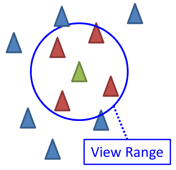
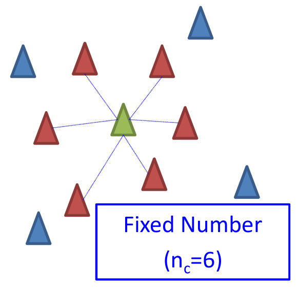
Figure 11: Two types of the definition for interacting neighbours. The left panel shows the metric definition, whereas the right panel corresponds to the topological definition. The number of mates interacting with a given arbitrary agent is $n_{c}=6$.

From now on, the model constructed by means of the metric definition of neighbours is referred to as metric model, whereas we call the model based on the topological definition as topological model.

In our topological modelling, we set the number of interacting mates $n_{c}=6$, which is suggested by empirical data analysis by Ballerini et. al. [14].

In order to construct the effective BOIDS simulation based on the topological definition of neighbours, we should introduce the following new types of interactions into our previous BOIDS.

1. Topological Cohesion: Making a vector of each agent’s position $\mbox{\boldmath$X$}_{i}\,(i=1,\cdots,N)$ toward the average position of neighbours in the topological sense, namely, the average position over the neighbouring mates up to the $n_{c}$-th nearest neighbour.

2. Global Cohesion: Making a vector of each agent’s position $\mbox{\boldmath$X$}_{i}\,(i=1,\cdots,N)$ toward the center of mass in the flocking in order to prevent the flock from splitting into more than two distinct clusters.

3. Topological Alignment: Keeping the velocity of each agent $\mbox{\boldmath$V$}_{i}\,(i=1,\cdots,N)$ the average value of topological neighbours (up to the $n_{c}$-th nearest neighbour).

We also slightly improve Separation as

1. Modified Separation: Making a vector of each agent to avoid the collision with mates up to the $n_{c}$-th nearest neighbour in the topological sense.

It is expected that the above Modified Separation enables us to avoid making regular-polygon structures in artificial flockings. Namely, in our previous BOIDS simulations, the regular-polygon structure might be induced by metrically defined Separation which acts for the only $1$-st nearest neighbour mate.

10.2 BOIDS dynamics

Hence, our topological model is described by the following update rules

$$\mbox{\boldmath$V$}_{i}(l+1) = \overline{V}_{l}^{(i)}\mbox{\boldmath$e$}_{B^{{}^{\prime}}}^{(i)}(l)$$ (24)

$$\mbox{\boldmath$X$}_{i}(l+1) = \mbox{\boldmath$X$}_{i}(l)+\mbox{\boldmath$V$}_{i}(l+1)$$ (25)

where $\mbox{\boldmath$e$}_{B^{{}^{\prime}}}(l)$ denotes a unit vector pointing to the direction to which the agent $i$ should move according to the above interactions of BOIDS and explicitly given by

$$\mbox{\boldmath$e$}_{B^{{}^{\prime}}}^{(i)}(l) = \frac{\frac{J_{1}\mbox{\boldmath$v$}_{\rm TC}^{(i)}(l)+J_{2}\mbox{\boldmath$v$}_{\rm TA}^{(i)}(l)+J_{3}\mbox{\boldmath$v$}_{\rm MS}^{(i)}(l)+J_{4}\mbox{\boldmath$v$}_{\rm GC}^{(i)}(l)}{|J_{1}\mbox{\boldmath$v$}_{\rm TC}^{(i)}(l)+J_{2}\mbox{\boldmath$v$}_{\rm TA}^{(i)}(l)+J_{3}\mbox{\boldmath$v$}_{\rm MS}^{(i)}(l)+J_{4}\mbox{\boldmath$v$}_{\rm GC}^{(i)}(l)|}+\eta\frac{\mbox{\boldmath$V$}_{i}(l)}{|\mbox{\boldmath$V$}_{i}(l)|}}{\left|\frac{J_{1}\mbox{\boldmath$v$}_{\rm TC}^{(i)}(l)+J_{2}\mbox{\boldmath$v$}_{\rm TA}^{(i)}(l)+J_{3}\mbox{\boldmath$v$}_{\rm MS}^{(i)}(l)+J_{4}\mbox{\boldmath$v$}_{\rm GC}^{(i)}(l)}{|J_{1}\mbox{\boldmath$v$}_{\rm TC}^{(i)}(l)+J_{2}\mbox{\boldmath$v$}_{\rm TA}^{(i)}(l)+J_{3}\mbox{\boldmath$v$}_{\rm MS}^{(i)}(l)+J_{4}\mbox{\boldmath$v$}_{\rm GC}^{(i)}(l)|}+\eta\frac{\mbox{\boldmath$V$}_{i}(l)}{|\mbox{\boldmath$V$}_{i}(l)|}\right|}$$ (26)

with

$$\mbox{\boldmath$v$}_{\rm TC}^{(i)}(l) = \frac{\frac{\sum_{j=1}^{N}\Theta(R_{n_{c}}^{(i)}-r_{ij})\mbox{\boldmath$X$}_{j}(l)}{|\sum_{j=1}^{N}\Theta(R_{n_{c}}^{(i)}-r_{ij})\mbox{\boldmath$X$}_{j}(l)|}-\mbox{\boldmath$X$}_{i}(l)}{\left|\frac{\sum_{j=1}^{N}\Theta(R_{n_{c}}^{(i)}-r_{ij})\mbox{\boldmath$X$}_{j}(l)}{|\sum_{j=1}^{N}\Theta(R_{n_{c}}^{(i)}-r_{ij})\mbox{\boldmath$X$}_{j}(l)|}-\mbox{\boldmath$X$}_{i}(l)\right|}$$ (27)

$$\mbox{\boldmath$v$}_{\rm A}^{(i)}(l) = \frac{\sum_{j=1}^{N}\Theta(R_{n_{c}}^{(i)}-r_{ij})\mbox{\boldmath$V$}_{j}(l)}{|\sum_{j=1}^{N}\Theta(R_{n_{c}}^{(i)}-r_{ij})\mbox{\boldmath$V$}_{j}(l)|}$$ (28)

$$\mbox{\boldmath$v$}_{\rm S}^{(i)}(l) = -\frac{\sum_{j=1}^{N}\Theta(R_{n_{c}}^{(i)}-r_{ij})(\mbox{\boldmath$X$}_{j}(l)-\mbox{\boldmath$X$}_{i}(l))}{|\sum_{j=1}^{N}\Theta(R_{n_{c}}^{(i)}-r_{ij})(\mbox{\boldmath$X$}_{j}(l)-\mbox{\boldmath$X$}_{i}(l))|}$$ (29)

$$\mbox{\boldmath$v$}_{\rm GC}^{(i)}(l) = \frac{\frac{\sum_{j=1}^{N}\mbox{\boldmath$X$}_{j}(l)}{|\sum_{j=1}^{N}\mbox{\boldmath$X$}_{j}(l)|}-\mbox{\boldmath$X$}_{i}(l)}{\left|\frac{\sum_{j=1}^{N}\mbox{\boldmath$X$}_{j}(l)}{|\sum_{j=1}^{N}\mbox{\boldmath$X$}_{j}(l)|}-\mbox{\boldmath$X$}_{i}(l)\right|}$$ (30)

where $R_{n_{c}}^{(i)}$ denotes the square distance between the agent $i$ and the $n_{c}$-th nearest neighbouring mate. Therefore, the number $n_{c}$ should be defined explicitly by

$$n_{c} = \sum_{j=1}^{N}\Theta(R_{n_{c}}^{(i)}-r_{ij})$$ (31)

for all $i$ because $\Theta(\cdots)$ survives only for the $j$ satisfying $r_{ij}<R_{n_{c}}^{(i)}$, and the number of such $j$ is just $n_{c}$ from the definition. The balance parameter $\eta$ is set to the same value $2$ as in the case of the metric model.

From the above definition of (27), we easily find that $\mbox{\boldmath$v$}_{\rm TC}^{(i)}(l)=-\mbox{\boldmath$v$}_{\rm MS}^{(i)}(l)$ and one of these two distinct effects is completely cancelled in the BOIDS dynamics (24)(25) as $\sim(J_{1}-J_{3})\mbox{\boldmath$v$}_{\rm TC}^{(i)}(l)$ for any choice of $J_{1},J_{3}$. To modify this undesirable situation, we slightly change the $\mbox{\boldmath$v$}_{\rm S}^{(i)}(l)$ as follows.

$$\mbox{\boldmath$v$}_{\rm MS}^{(i)}(l)=-\frac{\sum_{n=1}^{n_{c}}\Theta(R_{n}^{(i)}-r_{i\overline{j(n:i)}})(\mbox{\boldmath$X$}_{\overline{j(n:i)}}(l)-\mbox{\boldmath$X$}_{i}(l))}{|\sum_{n=1}^{n_{c}}\Theta(R_{n}^{(i)}-r_{i\overline{j(n:i)}})(\mbox{\boldmath$X$}_{\overline{j(n:i)}}(l)-\mbox{\boldmath$X$}_{i}(l))|}$$ (32)

where $\overline{j(i:n)}$ is given by the definition (18), and $R_{n}$ means the Separation Range for the $n$-th nearest neighbour mate.

From the empirical evidence [14], we set $R_{n}^{(i)}$ as

$$R_{n}^{(i)} = |r_{0}^{(i)}|n^{1/3}$$ (33)

where we define $R_{0}^{(i)}=R_{0}=0.73$ and $r_{0}^{(i)}$ is selected as a Gaussian variable with mean $R_{0}$ and unit variance.

From equation (24), we should notice that the amplitude of velocity vector of agent $i$ at time $l+1$ is identical to the average amplitude of velocity vectors for the topologically defined neighbouring mates, that is, the mates up to the $n_{c}$-th nearest neighbours in the previous time step $l$ as

$$|\mbox{\boldmath$V$}_{i}(l+1)| = \overline{V}_{l}^{(i)}\equiv\frac{\sum_{n=1}^{n_{c}}\Theta(R_{n}^{(i)}-r_{i\overline{j(i:n)}})|\mbox{\boldmath$V$}_{\overline{j(i:n)}}(l)|}{\sum_{n=1}^{n_{c}}\Theta(R_{n}^{(i)}-r_{i\overline{j(i:n)}})}.$$ (34)

The above update rules (24), (25), (26), (27), (28), (32) and (30) are our basic dynamical equations to be evaluated numerically.

We list a set of scale-lengths appearing in our simulations in Table 4. In both Table 1 (metric model) and Table 4 (topological model), we chose these scale-lengths from the empirical data [14]. However, we should keep in mind that the choices of $R_{0}$ are different in both cases. In the metric model, we used $R_{0}=1.09$ which is chosen from Event 29-03 in the reference [15], whereas $R_{0}=0.73$ in the topological model comes from Event 28-10 in [15].

A set of scale-lengths in the topological model
Number of agents ($N$)	100
Body-Length ($BL$)	0.2 [m]
Wing-Span ($WS$)	0.4 [m]
Radius of Separation Range ($R_{0}$)	0.73 [m]
Initial Speed Average $V^{{}^{\prime}}$	11.10 [m/s]
Initial Density of the Aggregation ($\rho$)	0.54 [${\rm m}^{-3}$]

Table 4: A set of scale-lengths in the topological model. Variables other than the Number of agents are based on empirical data by Ballerini et. al. (Event 28-10 in Table 1 of [15]).

For the topological model obtained by the above modifications, we utilize the GA to find the weights of the four interactions ((tc),(gc),(ta) and (ms)). Then, we numerically evaluate the $\gamma$-value and the the third-power of average distance ($R^{3}$) between an arbitrary agent and the $n$-th nearest neighbour as a function of order of neighbour $n$.

10.3 Results

We show the result in Fig.12. We plot the $\gamma$-value as a function of order $n$ (left panel) and the $R^{3}$ as a function of order of neighbour $n$ (right panel) for $n_{c}=6$.

In the left panel, we find that the anisotropy emerges ($\gamma>1/3$) up to $n_{c}=6$ and ‘anti-anisotropy’ disappears as we expected. From the right panel, we are also confirmed that the regular-polygon structures never emerges in the flock because the $R^{3}$ monotonically increases as the $n$ increases. Of course, here we used the empirical finding $R_{n}=R_{0}n^{1/3}$ [14] to determine the $R_{n}^{(i)}$ in the $\mbox{\boldmath$v$}_{\rm MS}^{(i)}(l)$ for our topological modelling, however, the result might justify that the flock in the metric model behaves as a ‘crystal form’, whereas the flock in the topological model looks like ‘gas’ which is much closer to real flockings.

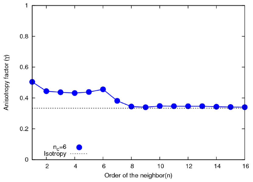
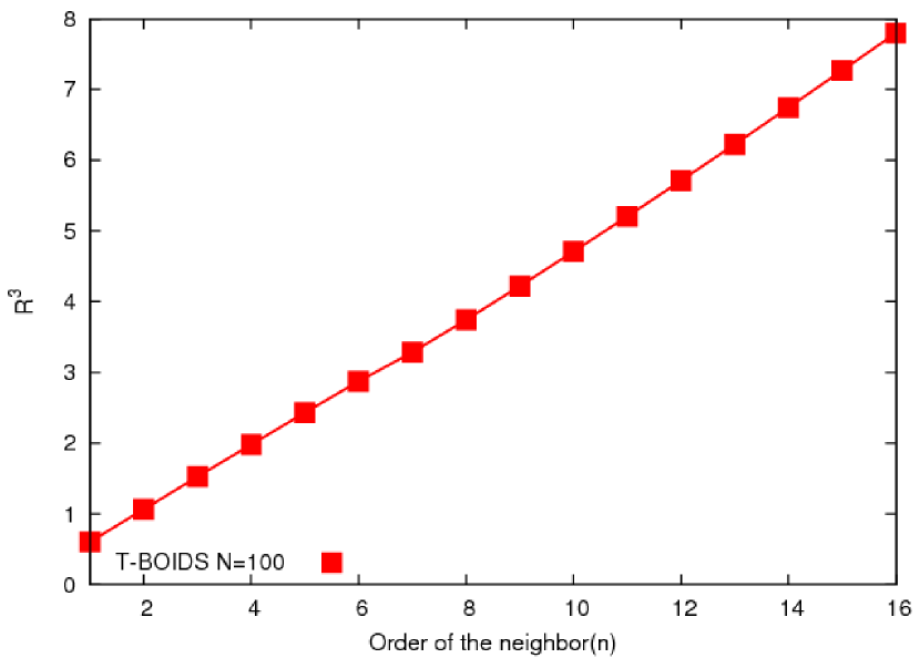
Figure 12: The resulting measurements for our topological model. The left panel shows the $\gamma$-value as a function of order $n$, whereas the right panel is plotted as third-power of average distance $R$ between an arbitrary agent and the $n$-th nearest neighbouring mate as a function of order of neighbour $n$. We set $n_{c}=6$, which is indicated by empirical evidence [14].

We also calculate the so-called integrated conditional density $\Gamma(r)$ and pair distribution function $g(r)$ introduced by Cavagna et. al. [24]. These two quantities are explicitly defined as

$$\Gamma(r) = \frac{1}{n_{c}}\sum_{i=1}^{n_{c}}\frac{N_{i}(r)}{4\pi r^{3}/3}$$ (35)

$$g(r) = \frac{1}{4\pi r^{2}}\frac{1}{n_{c}}\sum_{i=1}^{n_{c}}\sum_{j\neq i}\delta(r-r_{ij})$$ (36)

where $N_{i}(r)$ denotes the number of points in the sphere with the radius $r$ centered in $i$, and $n_{c}$ stands for the number of individuals in the sphere. $r_{ij}$ is the absolute distance between the center $i$ and the neighbour $j$. Here we should notice that these two quantities are related each other and satisfy

$$g(r) = \Gamma(r)+\frac{r}{3}\frac{d\Gamma(r)}{dr}.$$ (37)

Hence, we directly evaluated $\Gamma(r)$ from our simulations and calculated the $g(r)$ by means of the above equation.

We show the results in Fig. 13. From this figure, we find that both $\Gamma$ and $g$ for the metric model suddenly increase around the radius of view field $R_{0}=1.09$ and the behaviour is completely different from the empirical evidence [24]. On the other hand, these quantities for the topological model gradually increases around $r=0.4<R_{0}=0.73$ and the behaviour is very close to the empirical evidence (see Fig. 1 and Fig. 5 in [24]).

     

     

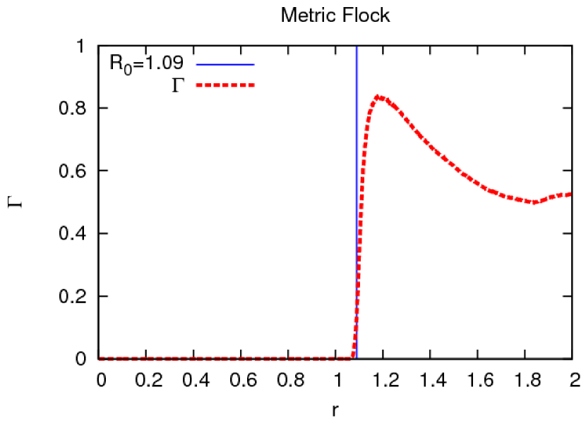
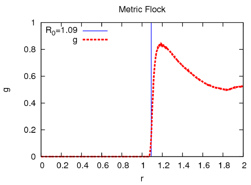
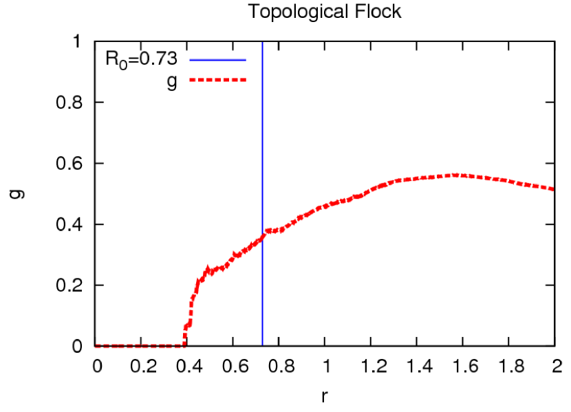
Figure 13: The integrated conditional density $\Gamma(r)$ (upper panels) and the pair distribution function $g(r)$ (lower panels) for the metric model (left panels) and the topological model (right panels).

From these numerical results, we conclude that our topological model reconstructs the essential features confirmed from empirical findings of starling. Although some tiny gaps have been left, for instance, the $\gamma$-value of the nearest neighbour is lower than the empirical evidence, one can say that our topological model is more likely to be ‘realistic’ than the metric model.

11 Discussion

In this section, we discuss several issues on our results.

11.1 On the optimal gene configuration

From Table 3, we find that the order of the strength of the weight $J_{1},J_{2}$ and $J_{3}$ is $J_{3}>J_{2}>J_{1}$ in any run of the GA. The condition $J_{3}>J_{1}$ is needed to require the ‘zero-collision’ constraint, whereas the condition $J_{3}>J_{2}>J_{1}$ makes the $\gamma$-value larger than that for the condition $J_{3}>J_{1}$. Actually, in our previous study [16], we carried out the simulations under the condition $J_{3}>J_{1}>J_{2}$, which was determined by hand, and found that the $\gamma$-value for $n=1$ is around $0.7$ which is apparently lower than the result of empirical findings $\gamma\simeq 0.8$ [14]. This fact is a reasonable advantage of our approach based on the GA to maximize the $\gamma$-value.

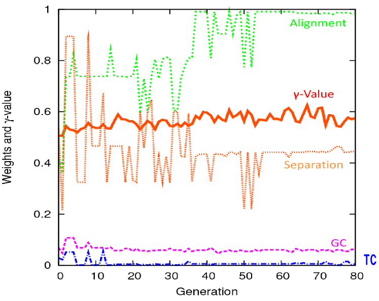
Figure 14: Evolution of $\gamma$-value in generations for the topological model.

On the other hand, for the topological model, we find the order of interactions as $J_{2}>J_{3}>J_{4}>J_{1}$ as shown in Fig. 14.

11.2 Theoretical upper bound of the $\gamma$-value

In our simulations, we used the $\gamma$ value as a ‘cost’ for the optimization problem to determine the three interactions in BOIDS. This procedure is possible because the $\gamma$-value itself is described as a function of these interactions implicitly, namely, $\gamma=\gamma(J_{1},J_{2},J_{3})$. Thus, by using the GA (the choice of GA as a tool to maximize it is not essential here, and of course, one can use the different methods such as simulated annealing), we maximized it under the ‘zero-collisions’ and ‘no breaking-up’ constraints. In this sense, this simple maximization process under two constraints leads to the empirical value of $\gamma$. Therefore, we might conclude that the flock is formed so as to maximize the $\gamma$-value and to satisfy the two constraints.

In fact, it is obvious from the definition that the upper bound of the $\gamma$-value is $1$. However, from the result shown in Table.3, the $\gamma$-value observed in our simulations is lower than the bound, namely, $\gamma\simeq 0.8$. We also examined to what extent the $\gamma$-value increases when we does not require any ‘zero-collision’ constraint during the GA dynamics and found that the $\gamma$ value increases up to near the bound. From these results we may conclude that the ‘zero-collision’ constraint reduces the $\gamma$-value considerably. However, we should notice that $\gamma$-value calculated in the empirical findings by Ballerini et. al. [14] also takes the value around $0.8$ which is very close to our result. Therefore, we might conclude that finding the optimal weights for the interaction by maximizing the $\gamma$-value under ‘zero-collision’ constraint is a reasonable way to realize more ‘realistic’ flocking simulations even in our personal computers.

Mathematically, inspired by the so-called Gardner’s capacity in the research field of neural networks [20], we might examine the following fraction of solution space:

$$\nu(\gamma)=\frac{\int_{0}^{\infty}d\mbox{\boldmath$J$}\Theta(|\mbox{\boldmath$J$}|-j)\delta(N_{\rm c})\delta(N_{\rm b})\delta(\gamma(\mbox{\boldmath$J$})-\gamma)}{\int_{0}^{\infty}d\mbox{\boldmath$J$}\Theta(|\mbox{\boldmath$J$}|-j)}$$ (38)

where $\Theta(\cdots)$ and $\delta(\cdots)$ stand for a step function and a delta function, respectively. Here we also defined $d\mbox{\boldmath$J$}\equiv dJ_{1}dJ_{2}dJ_{3}$, $\Theta(|\mbox{\boldmath$J$}|-j)\equiv\Theta(|J_{1}|-j_{1})\Theta(|J_{2}|-j_{2})\Theta(|J_{3}|-j_{3})$. $N_{c}$ and $N_{b}$ mean the numbers of collisions and breaking-up. Fixed constant variables $j_{k},k=1,2,3$ specify the supports for these three variables $J_{k},k=1,2,3$. The fraction $\nu$ might shrink (perhaps, monotonically) to zero when we increases the $\gamma$ and a ‘non-trivial’ theoretical upper bound $\gamma_{c}$ might be obtained as a solution of $\nu(\gamma_{c})=0$. In our forthcoming article, the details of this argument and the results will be reported.

11.3 Symmetry breaking in the space of interactions

In our BOIDS modelling, we gave the interactions such as $J_{1},J_{2}$ and $J_{3}$ for the metric model ($J_{1},J_{2},J_{3}$ and $J_{4}$ for the topological model) to all agents as the same values. However, of course, one could modify the situation so as to give the ‘agent-dependent interactions’ as $(J_{1}^{(i)},J_{2}^{(i)},J_{3}^{(i)})$ to the system. Then, it is very interesting for us to make two-dimensional histograms for each of the interactions like $J_{1}(\theta,\phi),J_{2}(\theta,\phi),J_{3}(\theta,\phi)$. From the histograms, we might obtain the useful information about the correlation (relationship) between anisotropy in position and anisotropy in the interaction. However, apparently the number of parameters to be determined by GA increases from three to $3N$ and the number (system size) is critical for our computational cost of determination by GA within a reliable precision and realistic computational time. Therefore, we would like to address this problem in our future studies.

11.4 Comparison with empirical findings

From Fig.8 and the same plot given by Ballerini et. al. [14], $\gamma$-values for $n=1$ are almost the same and the both decrease as $n$ increases. Moreover, these two curves (ours and Ballerini’s) converges to $1/3$ in the asymptotic limit of $n\to\infty$. However, in our evaluation, the $\gamma$-value becomes lower than $1/3$ in the range of $7\leq n\leq 14$, whereas the empirical evidence indicates $\gamma$-value monotonically decreases as $n$ increases and is saturated to $1/3$ beyond $n=6$. This is an essential difference between the Ballerini’s empirical findings and ours.

Here, we assume that the metric interaction might cause a regular-polygon structure (a locally crystallized structure) in the flocking leading up to the ‘anti-anisotropy’. Hence, in this paper, we also carried out the BOIDS simulations in which the neighbours for an arbitrary agent is defined topologically instead of metrically. We found that the anisotropy measurement does not show the anti-anisotropy and the gap between our modelling and empirical findings was actually reduced. However, the $\gamma$-value for $n=1$ is apparently smaller than the empirical evidence (see Fig.12 (left)) and it might be needed to introduce different types of constraints to design the artificial flocking in computers.

12 Summary

In this paper, we utilized GAs to maximize the $\gamma$-value in order to determine the weights for interactions in the BOIDS under ‘zero-collision’ and ‘no-breaking-up’ constraints. We found that this procedure enables us to simulate the realistic flocking phenomena even in our personal computer level. We showed that the resultant $\gamma$-value as a function of $n$-th order of the nearest neighbouring agents is quite similar to the empirical findings in several aspects [14, 21]. We carried out the simulations for both metric and topological definitions of neighbours in the flocking and found that the topological model reproduce the physical quantities of empirical evidence much better than the metric model does. Of course, there still exists a gap between the empirical evidence and our results by the BOIDS modelling. Recently, Bode et. al. [23] measured this anisotropy in artificial flockings by using stochastic, asynchronous updating scheme for each agent’s movement. Their model partially succeeded in reproducing the behaviour of the empirical findings and showed us a possibility that there exists more realistic flock simulations than the conventional deterministic one. In our modelling, such probabilistic ingredients were not taken into account, however, their numerical evidence might stress that such a stochastic agents is one of essential factors to generate much more realistic collective behaviour of flockings. The extensive studies to reduce the gap should be needed to reveal the nature of non-trivial collective behaviour in flocking phenomena.

Appendix

Appendix A Details of our genetic algorithm

We here explain our GA procedure in this paper as follows.

1. Initialization: Create gene configurations $U$.

2. Repeat the following procedure ($g=1:g\leq G$).

   1. Crossover: To make a crossover to generate a new gene configuration $E$.

   2. Mutation: Define a gene configuration $I=U+E$ and pick up $|I_{\rm s}|+|I_{\rm a}|$ components randomly from $I$ and mutate them.

   3. Selection: Select the gene configurations having high fitness values from $I$. We select such $|U|$ gene configurations and update the previous set $U$.

We next show the above Initialization more precisely as follows.

Initialization:

1. We give a random variable in the range $[0.001,0.999]$ to each gene $J_{1},J_{2}$ and $J_{3}$ and generate a gene configuration.

2. For the generated gene configuration, we evaluate the $\gamma$-value.

3. If the $\gamma$-value is no more than $\gamma_{\rm max}^{(0)}$ and any ‘collision’ or ‘breaking-up’ is not observed, we choose the $\gamma$-value as the fitness and add the corresponding gene configuration $(J_{1},J_{2},J_{3})$ to the set $U$.

4. Repeat the above (i1),(i2) and (i3) until the number of configurations reaches $|U|$.

Where we defined the $\gamma_{\rm max}^{(0)}$ to confirm that one can get optimal weights even if he (or her) starts the GA from wrong initial gene configurations having relatively low fitness values. We should keep in mind that the evaluation of $\gamma$-value is carried out for $8$-independent runs of simulations and we set the $\gamma$-value which is averaged over $8$-independent runs to the fitness function if and only if there is no ‘collision’ or ‘breaking-up’ during each trial.

We next explain the details of the Crossover.

Crossover:

1. Pick up arbitrary two gene configurations from the set $U$ and define these configurations as $a$ and $b$.

2. We swap arbitrary one gene in the $a$ for arbitrary one gene in the $b$.

3. We evaluate the $\gamma$-value for the modified $a,b$ and add them to the set $E$ if and only if there is no ‘collision’ or ‘breaking-up’.

4. Repeat the above procedures (c1),(c2) and (c3) until we have $|E|$ gene configurations.

As the searching (solution) space is constructed by only three variables $J_{1},J_{2}$ and $J_{3}$ having real numbers, it is naturally assumed that the effect of the crossover is relatively weak on the optimization by GAs. Thus, we overcome this weakness by introducing the following two kinds of Mutations.

Mutation

1. From the set $I\equiv U+E$, we pick up a gene configuration and define it as $c_{s}$.

2. We update arbitrary one gene, say, $J_{i}$, in the configuration $c_{s}$ randomly as $J_{i}\to J_{i}+\delta$, where $\delta$ stands for a random number in the range $[0.001,0.01]$.

3. For the modified $c_{s}$, we evaluate the $\gamma$-value and add the $c_{s}$ to the set $I$ if and only if there is no ‘collision’ or ‘breaking-up’.

4. Repeat the above (m1),(m2) and (m3) until we obtain $|I_{\rm s}|$ gene configurations.

5. We pick up an arbitrary gene configuration and replace a single gene $J_{i}$ with a random number in the range $[0.001,0.999]$. We make $|I_{\rm a}|$ gene configurations by making use of the same procedure and add the set $I_{\rm a}$ to the set $I$.

It should be noted that the above procedures (m1),(m2) and (m3) achieves ‘local search’ whereas the procedure (m5) acts as ‘global search’. Thus, the above Mutation realizes the effective searching by using a mixture of local and global searches.

Finally, we explain the details of the Selection as follows.

Selection

1. Pick up a gene configuration having the highest $\gamma$-value from the set $I$ as an elite and the evaluate the $\gamma$-value if and only if there is no ‘collision’ or ‘breaking-up’. Then, we add the gene configuration to the set $U$ in the next generation.

2. For all genes in the set $I$, we calculate the $\gamma$-values as the corresponding fitness values. If $g>G/2$, we make a linear transform on the $\gamma$-value for all gene configurations in the set $I$ and choose the transformed set of $\gamma$-values as fitness functions.

3. Make a roulette selection of the gene configuration based on the fitness functions and evaluate the $\gamma$-value if and only if there is no ‘collision’ or ‘breaking-up’. Then, we add the gene configuration to the set $U$ and repeat the above procedure until we have $|U|$ configurations.

As we are restricted ourselves to the case in which the number of trials, the time of observation are limited, there exists a possibility that we get unexpected high $\gamma$-value and the gene configuration having such high $\gamma$-value accidentally and to make matter worse, such gene configuration sometimes might survive until the final generation. To overcome this difficulty, we repeat the measurement of the $\gamma$-value for the selected gene configurations until ‘zero-collision’ condition is strictly satisfied and we delete the selected gene configurations if they lead to ‘collision’ or ‘breaking-up’ even if they show the high $\gamma$-value. Thus, we systematically solve the optimization problem under two essential constraints.

A.1 The size of GA in computer simulations

We next explain the size of GA in our computer simulations. We summarize them in Table 5.

Number of generation ($G$)	25
Size of gene configurations ($|U|$)	10
Initial $\gamma$-max	0.5
Crossover rate ($|E|$)	1
Mutation rate 1 ($|I_{\rm s}|$)	2
Mutation rate 2 ($|I_{\rm a}|$)	1

Table 5: Parameter setting for our GA.

We carry out the GA having the above setting-up of the parameters. Then, for each generation of the GA, we evaluate the $\gamma$-value, the weight of the interactions and the distribution of the gene configurations for three independent runs.

Appendix B Border bias effect and procedure to avoid it

In computer simulation for finite size systems ($N\ll\infty$), we should keep in mind that the results are sometimes influenced by the so-called border bias effect [22]. The border bias effect comes from the asymmetric shape of flockings. For instance, the asymmetric shape we mentioned here is typically an elliptical shape which is obtained as a deviation from a given symmetric sphere. The major axis of the elliptic corresponds to the direction of moving of the flock. For a given flocking and a given agent, the $n$-th nearest neighbouring agent is more likely to exist in the direction of moving of the flocking rather than the direction perpendicular to the flock’s movement. As the result, the $\gamma$-value decreases to below $1/3$ as $n$ increases, and then, ‘anti-anisotropy’ emerges. This phenomenon is nothing but border bias effect we mentioned here. It is very important for us to avoid the border bias effect to evaluate the $\gamma$-value precisely. If there is no correlation between the direction of flock’s moving and the shape of the flocking, one may cancel the effect by taking the average of the $\gamma$-value over several (usually, a lot of ) trials with different initial conditions. However, if not, it is very difficult for us to cancel the effect by this simple procedure. In most cases of simulations, the shape of flockings is an elliptic in which the major axis is always in the direction of flock’s moving and there exists an apparent correlation between the shape and the direction of moving. In general, the effect is more serious for the flocking simulation with small number of agents than that with huge number of agents. Ballerini and Cavagna et. al. cancelled the effect by excluding the agents on the border, however, the usefulness of their procedure is limited to the case in which the number of mates is larger than $400$ [14, 22].

From this fact in mind, we provide two distinct procedures to cancel the two types of border bias, namely, multiple trial method for border bias caused by ‘cubic shape’ (slab) of the flocking and sphere extraction method for border bias induced by ‘spherical shape’ of the flock. we show that these procedures make our flock simulations free from the border bias effects.

B.1 Multiple trial method

We first examine the extreme situation which shows ‘fake’-anisotropy by border bias [22].

Let us think about the artificial flocking having a cubic shape as shown in the left panel of Fig.15. The ratio of three slides of the cube is given as $7:3:1$. Then, we evaluate the $\gamma$-value for the flock moving to the direction of the shortest side. We also purposely make the flocking so as to show the isotropy for the angular distribution for individual by hand. Hence, we should naturally observe the ‘isotropy’ through the $\gamma$-value, namely, $\gamma=1/3$ if one correctly simulates the artificial flocking without any border bias effect.

The result is shown in the right panel of Fig. 15 by ‘circles’. From this panel, we clearly find that the anisotropy emerges and our simulations are apparently affected by the border bias. Even if we change the direction of flock’s motion from the shortest side to the longest slide, one cannot obtain the ‘isotropy’ but one observes the ‘anti-anisotropy’ as shown in the right panel of Fig. 15 by ‘boxes’.

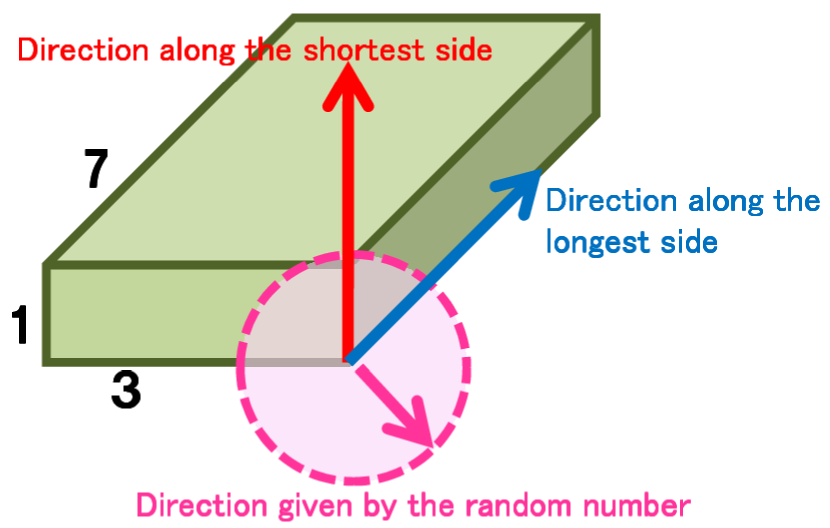
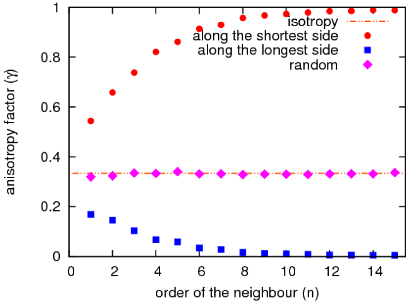
Figure 15: The extreme shape (‘cubic shape’) of artificial flocking which shows ‘fake’-anisotropy (left). The right panel shows the $\gamma$-value as a function of order $n$. Circles and boxes correspond to the $\gamma$-values observed in the flocking moving to the directions of the shortest and the longest sides, respectively. We purposely put $1200$-individuals randomly into this cubic so as to show the isotropy $\gamma=1/3$ by hand, however, the anisotropy/‘anti-anisotropy’ emerges. The ‘diamonds’ in this panel show the result by the multiple trial method. We clearly find that the isotropy is observed as we expected.

In order to overcome this type of border bias effects, we utilize the so-called multiple trial method. Namely, we evaluate the measurements such as the $\gamma$-value for a lot of independent trials, in each of which we give the initial direction of flock’s motion randomly without any correlations with any specific direction such as the shortest and the longest directions of cubic. Then, the measurement is obtained as an average over the trials. We show the resulting $\gamma$-value for $1000$-trials in the right panel of Fig. 15 by ‘diamonds’. We clearly find that the ‘isotropy’ is observed as we expected.

B.2 Sphere extraction method

In the previous subsection B.1, we were confirmed that the multiple trial method efficiently reduces the border bias effect. However, we should notice that the method is effective only for the case in which the direction of flock’s movement (specified by the velocity vector $V$) and the shape of the flocking has no correlation.

To understand it, let us define a unit vector pointing to the direction of the longest side of the cubic in the previous subsection B.1 by $\mbox{\boldmath$e$}_{L}$. Then, the following condition should be satisfied

$$\overline{\mbox{\boldmath$e$}_{L}\cdot\mbox{\boldmath$V$}} = 0$$ (39)

to use the multiple trial method effectively, where $\overline{(\cdots)}$ stands for the time average over the sampling from BOIDS dynamics. It is obviously confirmed when we consider the extreme case in which randomly given vectors $\mbox{\boldmath$V$}_{k}$ ($k=1,\cdots,M$: $M$ is the number of trials) as the direction of flock’s motion are always correlated with $\mbox{\boldmath$e$}_{L}$ in terms of $\overline{\mbox{\boldmath$e$}_{L}\cdot\mbox{\boldmath$V$}_{k}}=1\,(k=1,\cdots,M)$. For this case, we clearly notice that the multiple trial method gives exactly the same result as the ‘circles’ shown in the right panel of Fig. 15.

Therefore, another way to reduce the border bias effect is needed to evaluate the anisotropy measurement precisely in our BOIDS simulations.

In order to reduce the border bias effect in such cases, we take only agents who are in the sphere being inscribed with the shape of the flocking to calculate the $\gamma$-value. To check the usefulness of our procedure, we set-up $100$ agents moving with the same velocity in the same direction and give them their initial positions uniformly in the elliptic in which the major axis is in the direction of flock’s moving (see the inset of Fig. 16).

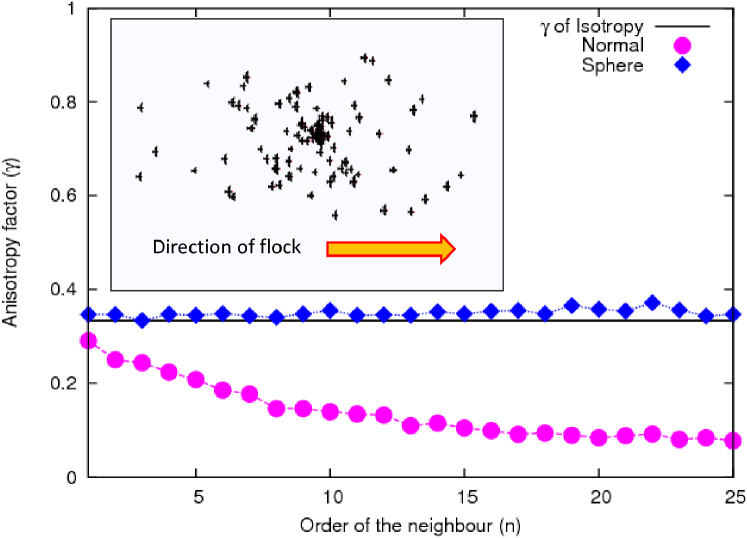
Figure 16: The $\gamma$-value as a function of order $n$. A typical snapshot of the aggregation is shown in the inset.

For these agents, we evaluate the $\gamma$-value up to $n=25$ and compare the result with the $\gamma$-value calculated without the above procedure. The results are shown in Fig.16. We carried out $1000$-independent runs and calculated the average of the $\gamma$-value. As we mentioned, the distribution of the position of agents is uniform and the correct (true) $\gamma$-value should be $1/3$. From this figure, we find that our procedure (circle Sphere) works well in comparison with the result without the procedure (diamond Normal).

References

- [1] Iwo Bialynicki-Birula and Iwona Bialynicka-Birula, Modeling Reality: How computers mirror life, Oxford University Press (2004).
- [2] Y. Inada, K. Kawachi, Order and flexibility in the motion of fish schools, J. of Theoretical Biology 214, pp.371-387 (2002).
- [3] A. Okubo Dynamical aspects of animal grouping: Swarms, schools, flocks, and herds, Advances in Biophysics 22, pp.1-94 (1986).
- [4] D.P. Landau and K. Binder, A Guide to Monte Carlo Simulations in Statistical Physics, Cambridge University Press (2005).
- [5] T. Vicsek, A. Czirk, E. Ben-Jacob, I. Cohen and O. Shochet, Novel type of phase transition in a system of self-driven particles, Physical Review Letters 75, pp.1226-1229 (1995).
- [6] C.W. Reynolds, Flocks, Herds, and Schools: A Distributed Behavioral Model, Computer Graphics 21, pp.25-34 (1987).
- [7] http://www.red3d.com/cwr/boids/
- [8] H. G. Tanner, A. Jadbabaie, and G. J. Pappas, Stable flocking of mobile agents, part I: Fixed topology, Proceedings of the 42nd IEEE Conference of DecisionControl, pp.2010- 2015 (2003).
- [9] H. G. Tanner, A. Jadbabaie, and G. J. Pappas, Stable flocking of mobile agents, part II: Dynamic topology, Proceedings of the 42nd IEEE Conference of DecisionControl, pp. 2016-2021 (2003).
- [10] R. Olfati-Saber, Flocking for Multi-Agent Dynamic Systems: Algorithms and Theory, IEEE Transactions on Automatic Control 51, No. 3, pp.401-420 (2006).
- [11] I. Aoki, A simulation study on the schooling mechanism in fish, Bulletin of the Japanese Society of Scientific Fisheries 48, pp.1081-1088 (1982).
- [12] H. Su, X. Wang, Z. Lin, Flocking of multi-agents with a virtual leader, IEEE Transactions on Automatic Control 54, No. 2, pp.293-307 (2009).
- [13] H. G. Tanner, A. Jadbabaie and G. J. Pappas, Flocking in Fixed and Switching Networks, IEEE Transactions on Automatic Control 52, No 5, pp.863-868 (2007).
- [14] M. Ballerini, N. Cabibbo, R. Candelier, A. Cavagna, E. Cisbani, I. Giardina, V. Lecomte, A. Orlandi, G. Parisi, A. Procaccini, M. Viale and V. Zdravkovic, Interaction Ruling Animal Collective Behaviour Depends on Topological rather than Metric Distance, Evidence from a Field Study, Proceedings of the National Academy of Sciences USA 105, No. 4, pp.1232-1237 (2008).
- [15] M. Ballerini, N. Cabibbo, R. Candelier, A. Cavagna, E. Cisbani, I. Giardina, A. Orlandi, G. Parisi, A. Procaccini, M. Viale and V. Zdravkovic, An empirical study of large, naturally occurring starling flocks: a benchmark in collective animal behaviour Animal Behaviour 76, pp.201-215 (2008).
- [16] M. Makiguchi and J. Inoue, Numerical Study on the Emergence of Anisotropy in Artificial Flocks: A BOIDS Modelling and Simulations of Empirical Findings, Proceedings of the Operational Research Society Simulation Workshop 2010 (SW10), CD-ROM, pp. 96-102 (the preprint version, arxiv:1004 3837) (2010).
- [17] P.A.M. Dirac, The principles of quantum mechanics , Clarendon Press, Oxford (1930).
- [18] D. E. Goldberg, Genetic Algorithms in Search, Optimization and Machine Learning, Addison Wesley (1989).
- [19] Y-W. Chen, K. Kobayashi, H. Kawabayashi and X. Huang, Application of Interactive Genetic Algorithms to Boid Model Based Artificial Fish Schools. Lecture Notes in Artificial Intelligence, Springer 5178, pp.141-148 (2008).
- [20] E. Gardner, The space of interactions in neural network models, Journal of Physics A: Mathematical and General 21, pp.257-270 (1988).
- [21] A. Cavagna, A. Cimarelli, I. Giardina, G. Parisi, R. Santagati, F. Stefanini and M. Viale, Scale-free correlations in starling flocks, Proceedings of the National Academy of Sciences USA 107, No. 26, pp. 11865-11870 (2010).
- [22] A. Cavagna, I. Giardina, A. Orlandi, G. Parisi, A. Procaccini, M. Viale and V. Zdravkovic, The STARFLAG handbook on collective animal behaviour: Part II, Animal Behaviour 76, Issue 1, pp.237-248 (2008).
- [23] N.W.F. Bode, D.W. Franks and A. Jamie Wood, Limited interactions are necessary for realistic movement in animal groups, Proceedings of the Royal Society Interfaces, published online before print September 8, 2010, doi:10.1098/rsif.2010.0397 (2010).
- [24] A. Cavagna, A. Cimarelli, I. Giardina, A. Orlandi, G. Parisi, A. Procaccini, R. Santagati and F. Stefanini, New statistical tools for analyzing the structure of animal groups, Mathematical Biosciences 214, pp.32-37 (2008).