Binaries migrating in a gaseous disk: Where are the Galactic center binaries?

Abstract

The massive stars in the Galactic center inner arcsecond share analogous properties with the so-called Hot Jupiters. Most of these young stars have highly eccentric orbits, and were probably not formed in-situ. It has been proposed that these stars acquired their current orbits from the tidal disruption of compact massive binaries scattered toward the proximity of the central supermassive black hole. Assuming a binary star formed in a thin gaseous disk beyond $0.1$ pc from the central object, we investigate the relevance of disk–satellite interactions to harden the binding energy of the binary, and to drive its inward migration. A massive, equal-mass binary star is found to become more tightly wound as it migrates inwards toward the central black hole. The migration timescale is very similar to that of a single-star satellite of the same mass. The binary’s hardening is caused by the formation of spiral tails lagging the stars inside the binary’s Hill radius. We show that the hardening timescale is mostly determined by the mass of gas inside the binary’s Hill radius, and that it is much shorter than the migration timescale. We discuss some implications of the binary’s hardening process. When the more massive (primary) components of close binaries eject most their mass through supernova explosion, their secondary stars may attain a range of eccentricities and inclinations. Such processes may provide an alternative unified scenario for the origin of the kinematic properties of the central cluster and S-stars in the Galactic center as well as the high velocity stars in the Galactic halo.

1. Introduction

The supermassive black hole (SMBH) in the Galactic center is surrounded by a parsec-scale cluster of young and massive stars. At separations larger than $\sim 1^{\prime\prime}$ or $0.04$ pc , about 100 OB stars are observed in a moderately thin disk that rotates clockwise on the sky and extends up to $\sim 0.6$ pc. The disk’s scale height to radius ratio is $\sim 0.1$. The stars have masses $\gtrsim 10\;M_{\odot}$ and a common age $\sim 6$ Myr. Their eccentricities range up to 0.8, with a typical value $\sim 0.4$ (e.g., Lu et al., 2009; Bartko et al., 2009, 2010). There is observational evidence for the existence of a second, less massive counter-clockwise disk comprising stars with similar age and kinematic properties as in the clockwise disk (Paumard et al., 2006; Bartko et al., 2009, 2010). In contrast, stars within the central arcsecond have orbits with random orientations and even higher eccentricities. Known as the “S-stars”, they are main-sequence B stars with masses of $\sim 10\;M_{\odot}$ and a lifespan of several $\times 10^{7}$ yrs (e.g., Schödel et al., 2002; Ghez et al., 2003; Bartko et al., 2010). The orbits of about $20$ of them have been determined by Gillessen et al. (2009). Their semi-major axes are as small as $\sim 4\times 10^{-3}$ pc $\approx 800$ AU, and their eccentricities are typically $\gtrsim 0.8$.

Explaining the presence of such young stars so close to the SMBH is challenging. The standard star formation scenario, invoking the collapse of self-gravitating cold molecular clouds, is unlikely to occur, because of the strong tidal perturbation from the SMBH (Morris, 1993). Nonetheless, the tidal disruption of a molecular cloud can form a thin accretion disk around the central object (Bonnell & Rice, 2008). In-situ star formation may then be triggered when the disk density is high enough so its self-gravity overcomes the tidal force of the SMBH (Levin & Beloborodov, 2003; Nayakshin & Cuadra, 2005), a process first predicted for the massive accretion disks present in AGNs (e.g., Kolykhalov & Syunyaev, 1980; Shlosman & Begelman, 1989; Goodman, 2003).

Alternatively, stars may have formed far from their current location and have migrated inwards due to dynamical friction. While the migration time for individual stars is much too long, a massive ($\gtrsim 10^{5}\;M_{\odot}$), dense stellar cluster formed several parsecs away could reach the central parsec in a few $10^{6}$ yrs (e.g., Gerhard, 2001). Both the self-gravitating disk scenario and the infalling cluster scenario can produce stellar disks (see Yu et al., 2007, and references therein), but the observed properties of the stellar disk in the central parsec favor in-situ formation (Nayakshin & Sunyaev, 2005; Paumard et al., 2006; Lu et al., 2009; Bartko et al., 2009).

Additional complexity arises when attempting to reproduce the peculiar orbits of the S-stars, which are even closer to the SMBH. The most promising mechanism involves the three-body interaction of a binary star and the SMBH (Hills, 1988). In particular, Gould & Quillen (2003) proposed that the S-stars were initially in compact binary systems. The binary can get tidally disrupted if it is scattered sufficiently close to the SMBH, such that its binary separation is a significant fraction of its Hill radius at its closest approach to the SMBH. In addition to potentially explaining the orbits of the S-stars, the binary’s tidal disruption scenario could account for the observed hypervelocity stars (Hills, 1988; Yu & Tremaine, 2003; Gualandris et al., 2005; Lu et al., 2007; Perets, 2009), most of which are B-type stars, just like the S-stars (e.g., Brown et al., 2007). In this context, Lu et al. (2010) and Zhang et al. (2010) have recently pointed out that the spatial distribution of the hypervelocity stars is consistent with being located on two thin disks. These authors have shown that this distribution could be reproduced by assuming that the hypervelocity stars originate from the tidal disruption of tight binaries initially located on two stellar disks near the Galactic center. In the tidal disruption scenario, one component of a compact binary is ejected at a velocity comparable to its orbital velocity around the binary’s center of mass, while the other component remains bound to the central black hole, with eccentricity and inclination very close to those of the binary’s center of mass before disruption. To produce bound B-type stars with eccentricities comparable to those of the S-stars, the original separation of the incoming binary (distance between both stars) would have to be $\sim 1$ AU (e.g., Gould & Quillen, 2003). Producing unbound B-type stars with ejection velocities $\sim 2000\;{\rm km\;s}^{-1}$ would demand an original separation typically $\lesssim 0.1$ AU (Hills, 1988; Bromley et al., 2006).

The presence of a couple of compact binary stars has been confirmed in the Galactic center (e.g., Martins et al., 2006). Several processes may account for their formation. The dynamic relaxation of a population of embedded single stars may lead to their capture into binary-star systems. Alternatively, binary stars may form during the fragmentation of a self-gravitating disk (Alexander et al., 2008a). But, these new born binaries generally have wide separations, and they are easily disrupted at large distance from the central black hole. The ejection speed of such disrupted binaries would generally be too small to produce either the hypervelocity stars or the large eccentricities of the S-stars. To do so, additional processes that can harden the binaries and drive their inward migration should be at work. Several stellar dynamical processes have been considered to bring the necessary binaries to the proximity of the SMBH (Perets et al., 2007; Löckmann et al., 2008; Madigan et al., 2009; Perets & Gualandris, 2010).

Interestingly, the S-stars have many properties analogous to the observed exoplanets, in particular the so-called Hot Jupiters. The latter are planets typically as massive as Jupiter, orbiting within $0.5$ AU from their host star. Some of these planets have eccentricities up to 0.97 (see e.g., Santos, 2008, for a recent review on exoplanets properties). According to planet formation theories, it is very unlikely to form a giant gaseous planet at such small distances from a star (Lin et al., 1996). Instead, giant planets are believed to form at larger separations in the protoplanetary gaseous disk surrounding the central object. The tidal interaction between the disk and the planet generally leads to decrease the planet’s semi-major axis (Ward, 1997). This is known as planetary migration. The migration of low-mass planets (say, an Earth-mass planet orbiting a solar mass star) has received considerable attention as it may occur on timescales much shorter than the lifetime of the protoplanetary disk (Tanaka et al., 2002), potentially bringing all these planets to the close proximity of their central host.

In the central parsec of our Galaxy, the star-to-supermassive black hole mass ratio is close to the Earth-to-Sun mass ratio. It suggests that “planet-like migration” could be an efficient way to bring young stars to the inner arcsecond (e.g., Artymowicz et al., 1993; Lin et al., 1994; Chang, 2008). Levin (2007) has proposed a scenario in which the S-stars formed in a sub-pc self-gravitating disk and migrated inwards by interacting with the disk. Because disk–satellite interactions damp the satellite’s eccentricities and inclinations on short timescales, an additional process is required to explain the large dispersion of the S-stars eccentricities and inclinations, like for the exoplanets. Levin (2007) proposed a fast resonant relaxation process that would randomize the S-stars’ eccentricity and inclination (Rauch & Tremaine, 1996). The presence of an intermediate-mass black hole may also influence stellar orbits, increasing their eccentricity and inclination considerably (Yu et al., 2007; Merritt et al., 2009; Gualandris & Merritt, 2009).

Our approach is to investigate the tidal interaction between a massive binary star and its parent gaseous disk as a mechanism to harden the binary, and to bring it to the SMBH proximity. This migration scenario differs from the stellar scattering scenario, where stars have parabolic encounters with the central black hole. The outline of this paper is the following. The physical properties of the system we model are described in § 2. We then discuss in § 3 the migration timescales we expect for a single star. The numerical set-up used in our hydrodynamical simulations is detailed in § 4. To alleviate the resolution requirements, we show in § 5 that it is possible to treat an equivalent rescaled problem. The calculation results obtained with the rescaled problem are presented in § 6. We then come back to our original problem in § 7, and we finally discuss our results in the context of the massive stars near the Galactic center in § 8.

2. Physical model

The system that we study comprises a supermassive black hole of mass $M_{\rm smbh}=3\times 10^{6}\;M_{\odot}$ surrounded by a gaseous disk, where stars are assumed to have already formed by disk fragmentation. For simplicity, only one satellite, a binary star, is embedded in the disk. Our aim is to investigate how disk–satellite interactions alter the orbital elements of the binary star (orbital migration, and possible evolution of the distance between both stars). The case of a single-star satellite with the same mass is also considered for comparison. The properties of the binary star and of the disk are described in § 2.1 and § 2.2.

2.1. Binary properties

We consider a binary with equal-mass stars. Both stars have a fixed mass $M_{\star}=15\;M_{\odot}$, akin to the star S0-2 orbiting Sgr A* (Martins et al., 2008). Gas accretion onto the stars is discarded. The satellite to primary mass ratio is $q=2M_{\star}/M_{\rm smbh}\sim 10^{-5}$, which is about three times the Earth-to-Sun mass ratio. The motion of the stars with respect to the binary’s center of mass is prograde. Results with a retrograde binary will also be presented in § 6.4. We denote by $a$ and $e$ the semi-major axis and eccentricity of the binary’s center of mass, with respect to the central black hole. The semi-major axis and eccentricity of the binary, with respect to its center of mass, are denoted as $a_{\rm bin}$ and $e_{\rm bin}$. We assume that the binary has initially $e=0$, $a=0.1\;{\rm pc}$, $e_{\rm bin}=0$, and $a_{\rm bin}=5\times 10^{-4}\;{\rm pc}\approx 100\;{\rm AU}$. The binary’s initial semi-major axis is thus $a_{\rm bin}=0.3R_{\rm H}$, where $R_{\rm H}=a\;(q/3)^{1/3}$ is the binary’s Hill radius.

2.2. Properties of the gaseous disk

The properties of gaseous disks around massive black holes prior to star formation have been described in many studies (e.g., Lin & Pringle, 1987; Levin, 2007). Such disks are expected to be geometrically thin, with a typical aspect ratio $h$ (ratio of the disk’s scale height $H$ to orbital radius $r$) between $0.5\%$ and $1\%$ (Nayakshin & Cuadra, 2005). But, investigating star–disk interactions requires knowledge of the disk properties after star formation, which are largely uncertain. The decrease of the disk density, and the increase of its temperature depend on the number and on the mass of stars formed (e.g., Shlosman & Begelman, 1989; Nayakshin, 2006; Nayakshin et al., 2007). We assume that the increase of the disk temperature after star formation is mild, and we set the disk aspect ratio to $h=1\%$ at $r=0.1\;{\rm pc}$ (the initial location of our binary-star system). This yields $R_{\rm H}\approx 1.5H$ at the binary’s initial location, which makes the two-dimensional approximation for the disk applicable in absence of gas accretion (D’Angelo et al., 2005). In addition, the fact $R_{\rm H}>H$ indicates that, despite its rather small mass, the binary may open a gap around its orbit, the depth of which depends on the disk’s turbulent viscosity around the binary’s orbit. The latter is modelled by a kinematic viscosity $\nu$. The gap-opening criterion takes the form (Lin & Papaloizou, 1993; Crida et al., 2006)

$$\frac{3}{4}\;h(a)\left(\frac{q}{3}\right)^{-1/3}+\frac{50\nu(a)}{q\;a^{2}\;\Omega(a)}\lesssim 1.$$ (1)

For our disk and binary parameters, the first term in Eq. (1) is $\approx 0.5$. Assuming $\nu=\alpha h^{2}a^{2}\Omega$ (Shakura & Sunyaev, 1973), the second term in Eq. (1) equals $50\alpha(a)h^{2}(a)/q$. Values of $\alpha$ in gravito-turbulent, critically fragmenting disks should typically range from $10^{-2}$ to $10^{-1}$ (e.g., Lin et al., 1988; Gammie, 2001; Lodato & Rice, 2004; Rafikov, 2009). Still, the value of $\alpha$ after star formation is uncertain, as stars modify the disk’s local properties (heating by shocks, gap-opening). For $\alpha(a)=10^{-2}$, the second term in Eq. (1) equals 5, suggesting the binary would slowly open a shallow gap. But, note that its actual value depends sensitively on $h(a)$. Given the uncertainties on both $h$ and $\alpha$, we assume that the viscosity at the binary’s location is low enough so that the binary rapidly clears a clean gap around its orbit. For this purpose, we take $\alpha(a)=10^{-3}$, and the second term in Eq. (1) equals 0.5.

We now describe the properties of the unperturbed disk before the satellite opens a gap. The disk’s angular velocity $\Omega$ is slightly sub-Keplerian, the gravitational force due to the central object being compensated for by the centrifugal force and by the pressure force. The temperature $T$ and surface density $\Sigma$ are set as power-law functions of $r$: $T(r)=T_{\rm 0.1\,pc}\,(r/{0.1\,\rm pc})^{-1}$, and $\Sigma(r)=\Sigma_{\rm 0.1\,pc}\,(r/{\rm 0.1\,pc})^{-1/2}$. Assuming a mean molecular weight $\mu=2.4$ and an adiabatic index $\gamma=5/3$, the initial temperature at $0.1$pc is $T_{\rm 0.1\,pc}\sim 2\times 10^{3}$K. The initial surface density at $0.1$ pc, $\Sigma_{\rm 0.1\,pc}$, is a free parameter in our study. It ranges from $\sim 20\;{\rm g\;cm}^{-2}$ to $\sim 200\;{\rm g\;cm}^{-2}$ for $Q_{\rm 0.1\,pc}$ between $1$ and $10$, where $Q_{\rm 0.1\,pc}$ stands for the Toomre parameter at $0.1$ pc,

$$Q_{\rm 0.1\,pc}=\left[\frac{c_{\rm s}\Omega}{\pi G\Sigma}\right]_{{\rm 0.1\,pc}},$$ (2)

with $c_{\rm s}$ the local sound speed. For simplicity, the gas self-gravity is neglected in our study.

If stars formed along the lines of the gravitational instability’s model, the disk is expected to be radiatively efficient in the stars forming region. After star formation, the increase of the gas temperature due to stellar heating, and the decrease of the gas density could significantly decrease the disk’s optical thickness (e.g., Bell & Lin, 1994). It is therefore possible that the gas becomes radiatively inefficient after star formation. Given again the uncertainties on the disk properties after star formation, we assume for simplicity that the gaseous disk is radiatively efficient, modeled with a locally isothermal equation of state (the initial temperature profile is maintained constant with time).

3. Migration timescale of a single star

We briefly review in this section the different regimes of migration resulting from the tidal interaction between a gaseous disk and a single-star satellite. A detailed review on disk–satellite interactions can be found in Masset (2008). Migration timescales are given assuming a two-dimensional disk with surface density and temperature profiles decreasing as $r^{-\sigma}$ and $r^{-\beta}$, respectively. The torque $\Gamma$ exerted by the disk on the satellite alters the satellite’s semi-major axis and eccentricity. Assuming the satellite is initially on a circular orbit, the time evolution of its semi-major axis $a$ is given by $2BqM_{\rm smbh}\;a\;\dot{a}=\Gamma$, where $B$ is the second Oort’s constant. The satellite’s migration timescale $\tau$ is defined as $\tau=|a/\dot{a}|$.

3.1. Type I migration

Type I migration applies to satellites that do not clear a gap around their orbit. The gap-opening criterion is recalled in Eq. (1). Assuming a disk aspect ratio at the star’s location of $\sim 1\%$ (see § 2.2), and a central object of a few $10^{6}$ solar masses, type I migration typically applies to stars up to a few solar masses. In this migration regime, the torque $\Gamma_{\rm I}$ exerted by the disk on the satellite is the sum of the differential Lindblad torque and of the horseshoe drag (Paardekooper & Papaloizou, 2009). The former accounts for the angular momentum carried away by the spiral density waves generated by the satellite, whereas the latter corresponds to the angular momentum exchanged between the satellite and the gas inside its corotation region (also known as horseshoe region). The total torque $\Gamma_{\rm I}$ can be written as

$$\Gamma_{\rm I}=-C_{\rm I}q^{2}\Sigma a^{4}\Omega^{2}h^{-2},$$ (3)

where all the unperturbed disk’s quantities in Eq. (3) are to be evaluated at the satellite location. The dimensionless factor $C_{\rm I}$ depends on $\sigma$, $\beta$, on the softening length of the satellite’s gravitational potential (required to adjust semi-analytic estimates of the horseshoe drag with the results of two-dimensional hydrodynamical simulations). It also depends on the properties of the gas disk, among which its self-gravity (Baruteau & Masset, 2008b), turbulent viscosity (Masset, 2001; Baruteau & Lin, 2010), and radiative properties (Baruteau & Masset, 2008a; Masset & Casoli, 2009; Paardekooper et al., 2010a, b). In a two-dimensional, non self-gravitating locally isothermal disk (see § 2.2), $C_{\rm I}$ can be approximated as $C_{\rm I}\approx 0.8+1.0\sigma+0.9\beta$ (Paardekooper et al., 2010a, their equation 49). For any density and temperature profiles decreasing with radius, $C_{\rm I}$ is positive, and type I migration is directed inwards. Using previous notations, the timescale for type I migration, $\tau_{\rm I}$, reads

$$\tau_{\rm I}\approx 4.3\times 10^{7}{\rm yrs}\times(0.8+1.0\sigma+0.9\beta)^{-1}\left(\frac{q}{3\times 10^{-6}}\right)^{-1}$$ (4)

$$\times \left(\frac{h}{10^{-2}}\right)\left(\frac{Q_{\rm 0.1\;pc}}{30}\right)\left(\frac{M_{\rm smbh}}{3\times 10^{6}\;M_{\odot}}\right)^{-\frac{1}{2}}\left(\frac{a}{\rm 0.1\;pc}\right)^{\sigma-\frac{\beta}{2}}.$$

In the particular case where $\sigma=2$ and $\beta=1$, Eq. (4) has the same dependence with the disk and satellite parameters as in equation (40) of Levin (2007). With our model parameters ($\sigma=1/2$, $\beta=1$, $h=10^{-2}$, $M_{\rm smbh}=3\times 10^{6}\;M_{\odot}$ and $a=0.1$ pc), and further assuming $q=10^{-7}$ ($R_{\rm H}\approx 0.3H)$ and $Q_{\rm 0.1\;pc}=3$, we find $\tau_{\rm I}\sim 6\times 10^{7}$ yrs $\approx 3.5\times 10^{4}$ orbital periods at $0.1\;{\rm pc}$. This timescale is slightly longer than the lifetime of the stars near the Galactic center. Note that $\sigma=1/2$ and $\beta=1$ make $\tau_{\rm I}$ independent of $a$. With $\sigma=2$ and $\beta=1$, $\tau_{\rm I}\propto a^{3/2}$ and goes down to a few $10^{6}$ yrs at $a\sim 0.01$ pc. Note also that, since $\tau_{\rm I}\propto q^{-1}$, more massive stars (but still subject to type I migration) will migrate faster. However, based on our thin disk assumption, the S-stars would open a gap around their orbit. They are therefore more likely subject to the slower type II migration. Still, it is possible that the S-stars have substantially migrated in before they acquired their asymptotic mass.

3.2. Type II migration

Type II migration concerns satellites that are massive enough to progressively deplete their horseshoe region, thereby opening a gap around their orbit. Assuming again a disk aspect ratio of $\sim 1\%$, and a central object of a few $10^{6}\;M_{\odot}$, type II migration typically applies to stars more massive than $\sim 10\;M_{\odot}$. Compared to the type I migration regime, the horseshoe drag is much reduced, and the Lindblad torque balances the viscous torque exerted by the disk. The total torque on the satellite can be written as a fraction $C_{\rm II}$ of the viscous torque due to the outer disk (Crida & Morbidelli, 2007, their equation 15). The factor $C_{\rm II}$ features the time-dependent fraction of gas $f_{\rm gas}$ left in the satellite’s horseshoe region.

The particular case where $f_{\rm gas}$ tends to zero is usually called the standard type II migration regime. Its timescale reads

$$\tau_{\rm II}\approx\frac{2r_{\rm o}^{2}}{3\nu(r_{\rm o})}\left(1+\frac{M_{\rm sat}}{4\pi\Sigma(r_{\rm o})r_{\rm o}^{2}}\right),$$ (5)

where $M_{\rm sat}=qM_{\rm smbh}$ denotes the satellite mass, and where $\Sigma$ is the density of the disk perturbed by the satellite. In Eq. (5), $r_{\rm o}$ is the location in the outer disk where most of the satellite’s angular momentum is deposited. It can be approximated as the location of the outer separatrix of the satellite’s horseshoe region, given by $r_{\rm o}\approx a+2.5R_{\rm H}$ for gap-opening satellites (Masset et al., 2006).

When the satellite mass is much smaller than the local disk mass $4\pi\Sigma(r_{\rm o})r_{\rm o}^{2}$, the type II migration timescale corresponds to the disk’s local viscous timescale (Lin & Papaloizou, 1986). In this regime, known as disk-dominated type II migration, the migration timescale $\tau_{\rm II,d}$ can be written as

$$\left.\tau_{\rm II,d}\right. \approx 1.8\times 10^{8}{\rm yrs}\times\left(\frac{\alpha}{10^{-2}}\right)^{-1}\left(\frac{h}{10^{-2}}\right)^{-2}$$ (6)

$$\times \left(\frac{M_{\rm smbh}}{3\times 10^{6}\;M_{\odot}}\right)^{-1/2}\left(\frac{r_{\rm o}}{\rm 0.1\;pc}\right)^{3/2},$$

where $\alpha$ and $h$ are to be evaluated at $r_{\rm o}$. This timescale is typically one order of magnitude longer than the timescale for type I migration, given in Eq. (4).

In the opposite case where the satellite mass is large compared to the local disk mass (satellite-dominated type II migration), the migration timescale $\tau_{\rm II,s}$ is

$$\tau_{\rm II,s}\approx\tau_{\rm II,d}\times\left(\frac{M_{\rm sat}}{4\pi\Sigma(r_{\rm o})r_{\rm o}^{2}}\right),$$ (7)

where the satellite to local disk mass ratio is

$$\left.\frac{M_{\rm sat}}{4\pi\Sigma(r_{\rm o})r_{\rm o}^{2}}\right. \approx 1.7\times 10^{-4}\left(\frac{M_{\rm sat}}{10\;M_{\odot}}\right)$$ (8)

$$\times \left(\frac{\Sigma(r_{\rm o})}{10^{2}\;{\rm g\;cm}^{-2}}\right)^{-1}\left(\frac{r_{\rm o}}{\rm 0.1\;pc}\right)^{-2}.$$

Eq. (8) shows that in the early stages of their formation and evolution, most of the massive stars near the Galactic center should be subject to the disk-dominated type II migration, and thus migrate in about the disk’s viscous timescale. Depletion of the gas disk, or substantial migration towards the central object, should however slow down migration as the stars inertial mass becomes comparable to the local disk mass.

3.3. Type III migration

Migrating satellites that open a partial gap experience an additional corotation torque due to fluid elements flowing across the horseshoe region (moving from the inner disk to the outer disk if the satellite migrates inwards). At small migration rates $\dot{a}$, this additional corotation torque is proportional to $\dot{a}$ (Masset & Papaloizou, 2003). When its amplitude is large enough, this torque may thus trigger a runaway migration. Runaway occurs, roughly speaking, when the mass deficit of the horseshoe region (the difference between the mass of the horseshoe region, and the mass that it would have if it had a uniform surface density equal to the density of the orbit-crossing flow) exceeds the satellite’s mass (Masset & Papaloizou, 2003). The occurrence and timescale of runaway migration, also referred to as type III migration, depend sensitively on the parameters entering the gap-opening criterion ($q$, $h$ and $\alpha$ at the satellite’s location), and on the disk mass (Masset & Papaloizou, 2003). It concerns intermediate-mass satellites (massive satellites clear a wide, deep gap, and the density of the orbit-crossing flow is too small to induce a significant mass deficit) in massive disks (the more massive the disk, the larger the density of the orbit-crossing flow). This migration regime could then be particularly relevant to $\gtrsim 3-10\;M_{\odot}$ stars embedded in thin ($h\sim 1\%$) massive ($Q\lesssim 10$) disks. Numerical simulations of disk–satellite interactions show that, depending on the resolution of the gas flow surrounding the satellite, the timescale for runaway migration may be as short as a few $10^{2}$ orbits (e.g., Masset & Papaloizou, 2003; Crida et al., 2009). It is thus possible that some of the massive stars near the Galactic center formed at separations $\geq 0.1$ pc, and reached the proximity of the central black hole through type III runaway migration.

4. Numerical model

4.1. Numerical method

All our calculations are performed with the two-dimensional code FARGO. It is a staggered mesh code that solves the Navier-Stokes and continuity equations on a polar grid. An upwind transport scheme is used along with a harmonic, second-order slope limiter (van Leer, 1977). Its main feature is to use a change of rotating frame on each ring of the grid, which increases the timestep significantly (Masset, 2000).

Our calculation results are expressed in the following units. The initial semi-major axis $a_{0}$ of the binary’s center of mass (or of the satellite if single) is the length unit, the mass of the central object $M_{\rm smbh}$ is the mass unit, and $(GM_{\rm smbh}/a_{0}^{3})^{-1/2}$ is the time unit, $G$ being the gravitational constant ($G=1$ in our unit system). Whenever time is expressed in orbital periods, it refers to as the orbital period of the binary’s center of mass (or of the satellite if single) around the central black hole.

We describe in this paragraph the numerical set-up of our calculations. Unless otherwise stated, the disk and satellite parameters are those described in § 2. Since our model assumes a locally isothermal disk, simulations do not include an energy equation (the temperature’s initial radial profile does not evolve with time). All calculations are performed in the frame corotating with the binary’s center of mass, or with the satellite if single. Wave-killing zones are used next to the grid’s inner and outer edges in order to minimize unphysical wave reflexions (de Val-Borro et al., 2006). In simulations with a binary satellite, we follow Cresswell & Nelson (2006) and set the timestep as the minimum value between the hydrodynamical timestep, and a fixed fraction of the binary’s internal orbital period,

$$\delta t_{\rm bin}=\frac{2\pi}{400}\;\left[\frac{d_{\rm bin}^{3}}{2GM_{\star}}\right]^{1/2},$$ (9)

where $d_{\rm bin}$ stands for the separation between the two stars. To avoid a violent initial evolution of the disk, the stars’ gravitational potential is slowly turned on over 10 orbital periods. Discussion on the form of the stars potential, and on the grid resolution follows in § 4.2.

4.2. Resolution issues

The time-evolution of the binary should sensitively depend on how the gas flow around and between the stars is resolved. As is usual in disk–satellite 2D hydrodynamical simulations, the stars potential is smoothed over a softening length $\varepsilon$. Two parameters therefore determine the resolution of our calculations: the grid’s resolution and the softening length of the stars potential. In this study, we choose a rather large value for $\varepsilon$ in order to prevent a large accumulation of gas around each star, which would otherwise require a prohibitively high grid’s resolution to be properly handled. The default value for $\varepsilon$ is half the binary’s initial semi-major axis $a_{\rm bin,0}$ (the same value is used in simulations with a single satellite). The softening length is therefore kept constant throughout the simulation. Smaller values of $\varepsilon$ will be considered in § 6.3.

We aim to resolve the satellite’s Hill radius with about 50 cells along the radial and azimuthal directions (Crida et al., 2009). This requirement implies a maximum size for the grid cells equal to $\delta_{\rm max}=0.02R_{\rm H}\approx 3\times 10^{-4}a$. To model the global disk–satellite interaction, it is enough to set the grid’s radial extent to $\Delta r=15R_{\rm H}$. This sets the number of cells along the radial direction to $N_{\rm r}=750$. The cell number along the azimuthal direction is then $N_{\rm s}=2\pi a/\delta_{\rm max}\approx 21000$. In contrast to $N_{\rm r}$, the value of $N_{\rm s}$ is about one order of magnitude larger than its typical value in 2D hydrodynamical simulations of disk–satellite interactions. To maintain a reasonable computational cost, we show in § 5 that it is possible to transform our problem into an equivalent rescaled problem, less computationally demanding, by making use of the dimensionless parameters in the gap-opening criterion at Eq. (1).

5. Rescaled problem

Table 1Parameters of the calculations of § 5, where the rescaling method is illustrated. All runs have the same values for $d_{1}=q/h^{3}$ and $d_{2}=qa^{2}\Omega/\nu$, the dimensionless quantities entering the gap-opening criterion.

Parameter	Run a	Run b	Run c
$h$	$1\%$	$3\%$	$5\%$
$q\propto h^{3}$	$8\times 10^{-6}$	$2.2\times 10^{-4}$	$10^{-3}$
$\nu/a^{2}\Omega\propto q$	$8\times 10^{-8}$	$2.2\times 10^{-6}$	$10^{-5}$
$\alpha=\nu/h^{2}a^{2}\Omega$	$8\times 10^{-4}$	$2.4\times 10^{-3}$	$4\times 10^{-3}$
$R_{\rm H}/a\propto h$	$1.4\%$	$4.2\%$	$6.9\%$
$r_{\rm min},r_{\rm max}$	$0.88,1.16$	$0.64,1.48$	$0.4,1.8$
$N_{\rm r},N_{\rm s}$	$448,6700$	$448,2238$	$448,1344$

Figure 1.— Results of the calculations of § 5, whose main parameters are summed up in Table 1. Left: azimuthally-averaged density profiles at $3000$ orbits. The azimuthal averaging excludes the disk parts located less than a few Hill radii away from the satellite. The x-axis displays the disk–satellite radial distance $\Delta$, in units of the satellite’s Hill radius. The initial surface density at the satellite’s location equals $10^{-4}$ in code units. Right: time evolution of the specific torque exerted by the disk on the satellite.

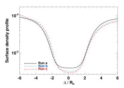
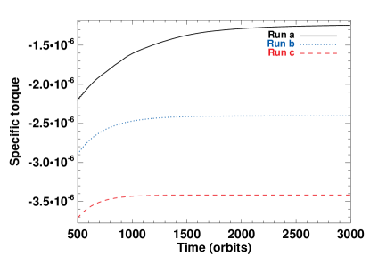
For a single satellite with fixed semi-major axis $a$, the gap-opening criterion involves two dimensionless quantities: $d_{1}=q/h^{3}$ and $d_{2}=qa^{2}\Omega/\nu$. Any changes of $q$, $h$ and $\nu$ that keep $d_{1}$ and $d_{2}$ constant will preserve the gap’s density profile (width, depth) in scaled units $\Delta/R_{\rm H}$, where $\Delta$ stands for the disk–satellite radial distance (Crida et al., 2006). The major resolution issue pointed out in § 4.2 is due to the fact $N_{\rm s}\propto{R_{\rm H}}^{-1}\propto q^{-1/3}$. Rising $q$, while keeping $d_{1}$ and $d_{2}$ constant, allows decreasing $N_{\rm s}$ while maintaining the same gap properties. We illustrate this result for a single satellite with a series of three calculations, referred to as Runs a, b, and c. In all three models, $d_{1}=8$ and $d_{2}=100$. The main parameters of these runs are summarized in Table 1. The disk aspect ratio increases from $h=1\%$ (Run a) to $h=5\%$ (Run c), which comes to increase the satellite to primary mass ratio $q$ and the kinematic viscosity $\nu$ by about two orders of magnitude. All runs have $N_{\rm r}=448$. The location of the grid’s inner and outer edges, $r_{\rm min}$ and $r_{\rm max}$, is adjusted such that $\Delta r=r_{\rm max}-r_{\rm min}=20R_{\rm H}$ ($\delta_{\rm max}/R_{\rm H}=4.5\%$). The number of cells along the azimuthal direction is taken as $N_{\rm s}=4\pi a/3\delta_{\rm max}$, it is thus $\approx 5$ times smaller in Run c than in Run a. In all these runs, the satellite is held on a fixed circular orbit in order to focus on the gap properties at a given semi-major axis. The initial disk density at the satellite location is $10^{-4}$ in code units. Since the gas self-gravity is neglected, and the satellite is on a fixed orbit, the gas density value can be chosen arbitrarily.

Azimuthally-averaged density profiles at $3000$ orbits are plotted against $\Delta/R_{\rm H}$ in the left panel of Figure 1. At a given radius, azimuthal averages exclude the disk parts located less than a few Hill radii away from the satellite. In scaled units $\Delta/R_{\rm H}$, the width and depth of the gaps are in good agreement. Although not shown here, we also checked that the density distribution inside the satellite’s Hill radius is almost indistinguishable from one calculation to another. This is an important point to keep in mind since, as will be shown below, the evolution of binary satellites is primarily driven by the density distribution in the satellite’s Hill radius.

We display in the right panel of Figure 1 the time evolution of the specific torque (torque per unit satellite mass) exerted by the disk on the satellite, for our series of three runs. The specific torques differ by a factor of order unity. The slight increase of the torque amplitude from Run a to Run c stems from the fact (i) the surface density at the outer horseshoe separatrix, namely at $\Delta\approx 2R_{\rm H}$, takes very similar values in all runs, whereas (ii) the density of gas left in the gap, which notably contributes to the positive horseshoe drag, slightly decreases from Run a to Run c (Crida & Morbidelli, 2007, their equation 15). We comment that the timescale to reach a steady-state varies between the simulations, which results from different gap’s depletion timescales. A gap progressively deepens as fluid elements leave the satellite’s horseshoe region. The timescale to build up a stationary gap profile is therefore proportional to the libration period of the horseshoe fluid elements,

$$\tau_{\rm lib}\approx\frac{8\pi a}{3\Omega x_{\rm s}},$$ (10)

where $x_{\rm s}$ is the half-width of the horseshoe region. For large values of the dimensionless parameter $q/h^{3}$, $x_{\rm s}\approx 2R_{\rm H}\propto q^{1/3}$ (see e.g., Masset et al., 2006). The timescale to get a stationary gap profile thus decreases with increasing $q$, and it should scale with $h^{-1}$. This is in good agreement with our results. The torques differ indeed by 5% from their final value at about $2000$ orbits for Run a, $1000$ orbits for Run b, and $600$ orbits for Run a. This comparison shows that, not only our rescaling method allows reducing the simulations computational cost, it also helps to reach a faster steady-state, while getting very similar results in terms of the density distribution and specific torque.

6. Results of calculations of the rescaled problem

We have shown in § 5 that the original problem described in § 2 can be transformed into an equivalent, less computationally demanding rescaled problem, by using the two dimensionless parameters in the gap-opening criterion. By equivalent, we mean that the properties of the gap opened by the satellite (width, depth), and thus the value of the specific torque on the satellite are fairly preserved with the rescaling method. This result was shown for a single satellite. We will show in § 6.1 that the gap properties of single and binary satellites are in good agreement, allowing us to apply the rescaling method to binary satellites. All the calculation results presented in this section therefore use the rescaling method. We come back to our original problem in § 7.

Before presenting our results, we briefly enumerate the parameters of the rescaled problem that we tackle in this section. The satellite to primary mass ratio is $q=10^{-3}$, and the disk aspect ratio at the satellite location is $h(a)=5\%$. The disk’s kinematic viscosity is constant, its value can be related to an equivalent alpha parameter at the satellite location $\alpha(a)=4\times 10^{-3}$. As shown in § 5, this set of parameters gives similar results (gap properties, specific torque on a single satellite) to that of our original, Galactic-center motivated problem in § 2: $q=10^{-5}$, $h(a)\lesssim 1.1\%$, and $\alpha(a)=10^{-3}$. The initial surface density at the satellite location is $10^{-4}$ in code units. The initial Toomre parameter at the binary’s location $\sim 160$, but (much) smaller values will be investigated in § 6.3. The grid now includes $N_{\rm r}=800$ rings and $N_{\rm s}=3000$ sectors, and it extends from $r_{\rm min}=0.55a$ to $r_{\rm max}=1.6a$ along the radial direction. The satellite’s Hill radius is resolved by about 50 cells along the radial direction, and by about 33 cells along the azimuthal direction. Initially, the binary’s semi-major axis is $a_{\rm bin,0}=2\times 10^{-2}\;a_{0}\approx 0.3R_{\rm H}$. The softening length of the stars potential is $\varepsilon=a_{\rm bin,0}/2$, and, to avoid a violent initial evolution, the mass of the binary stars is slowly increased until it reaches its proper value at 10 orbital periods.

Our calculations are performed in two steps. The satellite is first held on a fixed circular orbit for $500$ orbits, during which the satellite opens a gap. During this stage, the force exerted by the disk on the satellite is ignored. Both the quantities $a$ and $a_{\rm bin}$ therefore remain stationary during this first stage. Because initially $a_{\rm bin}=0.3R_{\rm H}$, the increase of the binary’s eccentricity due to the central star remains small (on average, $e_{\rm bin}\sim 0.04$). After $500$ orbits, the force exerted by the disk on the satellite is included, inducing the satellite’s orbital evolution. For comparison, calculations were performed both with a binary and a single satellites of the same $q$.

6.1. Binary satellite on a fixed circular orbit

Figure 2.— Calculation result of the rescaled problem ($q=10^{-3}$, $h=5\%$, $\alpha=4\times 10^{-3}$). Top-left: surface density contour at $500$ orbits of the gaseous disk surrounding the supermassive black hole, located at $x=0$, $y=0$. The binary’s center of mass is located at $x=1$, $y=0$. Top-right: close-up of the density distribution around the binary (note that polar coordinates are used in this panel, the binary’s center of mass is located at $r=r_{\rm b}$, $\varphi=\varphi_{\rm b}$). The dashed circle shows the binary’s Hill radius. Part of the computational grid is overplotted in the bottom-left part of the panel. The bottom panels show a sequential time evolution of the disk density in the binary’s Hill radius over almost half a revolution of the stars around their center of mass (which corresponds to about 0.05 orbital periods around the central black hole). The color scale and the axes are the same as in the top-right panel.

Figure 3.— Left: surface density profile time-averaged over the $500$ orbits the satellite is held on a fixed circular orbit. In contrast to the left panel of Figure 1, the azimuthal averaging takes into account the full azimuthal extent of the grid. The bottom x-axis displays the disk–satellite radial distance $\Delta$, in units of the satellite’s Hill radius. The top x-axis shows the separation from the central object. Right: running-time averaged specific torque exerted on each satellite (the two stars in the binary satellite case). Time is given in orbital periods of the satellite around the central black hole.

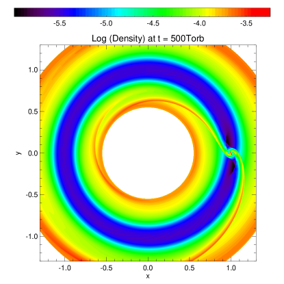
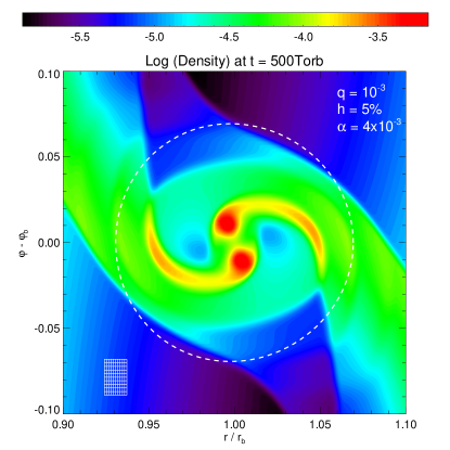
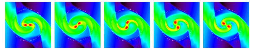
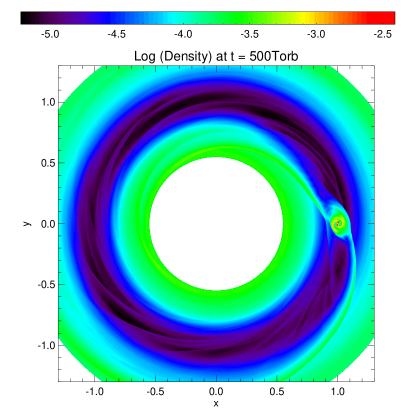
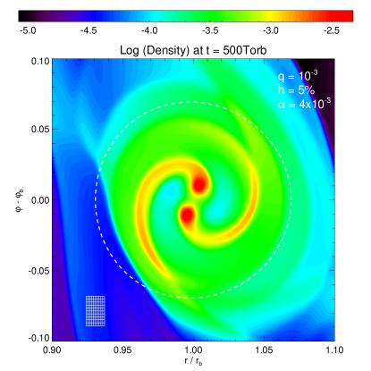
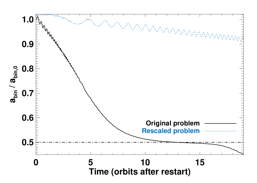
We describe in this paragraph the results obtained in the first $500$ orbits the binary satellite is held on a fixed circular orbit. The disk surface density obtained at $500$ orbits is displayed in the top-left panel of Figure 2. The central object is located at $x=0$, $y=0$, the binary’s center of mass is at $x=1$, $y=0$. A close-up on the density distribution around the binary is shown in the top-right panel of Figure 2. The stars are located at the center of the two densest points in this plot. The dashed circle depicts the satellite’s Hill radius, the size of which is $\approx 1.4H(a)$. Part of the computational grid is displayed in the bottom-left part of this panel. The binary is prograde, stars thus rotate counterclockwise in this panel. We see that each star is lagged by a spiral wake (or tail). The impact of these wakes on the binary’s orbital evolution is presented in § 6.2. The bottom panels in Figure 2 display a time evolution sequence of the density inside the binary’s Hill radius during almost half a revolution of the stars around their center of mass (that is during $\approx 0.05$ orbital periods around the central black hole). The color scale and the axes are identical as in the top-right panel of this figure. This sequence shows that the density in the trailing tails is strengthened as the stars cross the tidal wake induced by the binary’s center of mass. This density enhancement arises from a larger velocity difference between the stars and the gas at the location of the tidal wake.

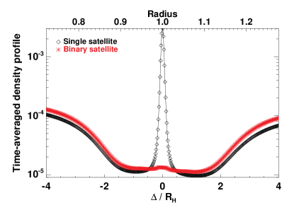
Far enough from the binary’s Hill radius, the disk density much resembles the typical disk density obtained with a single satellite, as expected (the quadrupole component of the binary’s potential becomes negligibly small compared to the monopole outside of the binary’s Hill radius). The left panel of Figure 3 compares the time-averaged surface density profiles obtained with the single and binary satellites. Time-averaging is done over the $500$ orbits of the simulations. In contrast to the left panel of Figure 1, the azimuthal averaging does not discard the material close to the satellite’s location. This is meant to highlight that the disk mass in the vicinity of the single satellite is about two orders of magnitude larger than the one around the binary. In the binary case, the fast relative motion of the stars and of the background gas hinders gas accumulation inside the satellite’s Hill radius. This is in contrast to the single satellite, where a massive circum-satellite disk forms inside the Hill radius (see e.g., Crida et al., 2009). Despite the large mass difference inside the Hill radius, the width and depth of the gaps opened by the single and binary satellites are in good agreement.

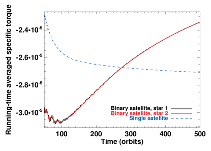
The right panel of Figure 3 displays the running-time averaged specific torque exerted on each star of the binary system (solid curves). Recall that time is in units of the satellite’s orbital period around the black hole (as in all other figures). Both torques are indistinguishable. For comparison, the running-time averaged specific torque on the single satellite is also shown (dashed curve). At $500$ orbits, the torque obtained in the binary case is about $10\%$ more positive, which results from a slightly less depleted gap, as illustrated in the left panel of Figure 3. In addition, we notice from the time evolution of the torques that the gap’s depletion timescale takes somewhat longer with a binary satellite. In particular, the running-time averaged torque on the binary has not reached a steady-state at $500$ orbits. We will show in § 6.3 that it does not change our results for the binary’s orbital evolution.

6.2. Binary’s orbital evolution

Figure 4.— Orbital evolution of the binary star in its parent gaseous disk. The top panel shows the semi-major axis $a$ of the binary’s center of mass (solid curve). The calculation result with a single satellite is overplotted for comparison (dashed curve). The binary’s semi-major axis $a_{\rm bin}$ is displayed in the middle panel. The calculation was halted when the separation between the binary stars became approximately smaller than the stars softening length, depicted as an horizontal dash-dotted line in this panel. Recall that both $a$ and $a_{\rm bin}$ are expressed in units of $a_{0}$, the value of $a$ before restart. The binary’s eccentricity $e_{\rm bin}$ is shown in the bottom panel.

Figure 5.— Impact of the disk’s density distribution inside the binary’s Hill radius on its hardening. We show the result of four runs restarted from the simulation of § 6.1. In these four runs, the calculation of the force (or the torque) exerted by the disk on the binary stars excludes a fraction $f$ of the binary’s Hill radius $R_{\rm H}$ (centered on the binary’s center of mass). The fraction $f$ equals $0$, $1/4$, $1/2$ and $1$ from bottom to top. The particular case with no material exclusion ($f=0$) corresponds to the calculation results shown in Figure 4. When the torque exerted by all the fluid elements in the binary’s Hill radius is discarded ($f=1$), the binary does not harden with time. The semi-major axis of the binary’s center of mass is displayed in the inset plot for all four calculations.

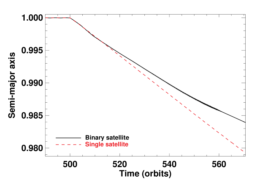
The simulation presented in § 6.1 was restarted at $500$ orbits, allowing the binary stars to feel the force exerted by the disk. As previously, we compare calculation results of single and binary satellites. The semi-major axis of the binary’s center of mass (solid curve), and of the single satellite (dashed curve) are displayed in the top panel of Figure 4. Both the single and binary satellites migrate inward. The binary’s migration rate is slightly smaller, however, and it tends to decrease with time. This behavior is consistent with the slow decrease of the running-time averaged specific torque shown in the right panel of Figure 3, and is due to the minor differences in the gas density profiles depicted in the left panel of Figure 3. Extrapolating the results in the top panel of Figure 4, we find that the migration timescale of the binary’s center of mass is about $5000$ orbits, or $\sim 8\times 10^{6}$ yrs at $0.1$ pc. This is about a factor of $2$ shorter than the prediction of Eq. (6), which however estimates the minimum timescale expected in the type II migration regime. We have checked that this discrepancy arises from the torque exerted by the circum-satellite disk inside of the satellite’s Hill radius. Another restart run with the single satellite, wherein the calculation of the force exerted on the satellite excludes the disk material inside of the satellite’s Hill radius, gives a migration rate that is about half that of the simulation shown in the top panel of Figure 4, and which is thus consistent with the pace expected in the disk-dominated type II migration regime. This behavior is further commented and illustrated for the binary satellite in the inset panel of Figure 5.

As shown in the middle panel of Figure 4, the binary’s semi-major axis $a_{\rm bin}$ decreases with time. We observe that the amplitude of the hardening rate, namely the quantity $|\dot{a}_{\rm bin}|$, slowly increases with time. The calculation was stopped when the separation between both stars went slightly below the softening length $\varepsilon=a_{\rm bin,0}/2$, depicted as a dash-dotted line in this panel. Below this separation, the binary satellite mostly interacts with the surrounding disk like a single-star satellite. In particular, we have checked that a massive, circular circumbinary disk starts to form around both stars, like with a single-star satellite. Our calculation result indicates that the binary’s semi-major axis is reduced by a factor of $2$ in $\approx 70$ orbits around the central black hole, or in about $1000$ orbits of the stars around their center of mass. This corresponds to $\sim 10^{5}$ yrs at $0.1$ pc in the Galactic center case. In this particular simulation, the hardening timescale of the binary is $\sim 40$ times shorter than its migration timescale.

The bottom panel of Figure 4 shows the time evolution of the binary’s eccentricity $e_{\rm bin}$. The interaction with the gas slowly decreases both the averaged value, and the amplitude of the eccentricity’s oscillations. Although not shown here, we have checked that the eccentricity of the binary’s center of mass remains negligibly small with time.

The binary’s hardening results from the formation of a spiral tail at the trailing side of each star (Escala et al., 2004; Kim et al., 2008; Stahler, 2010). Kim et al. (2008) showed that each perturber is dragged backward by its own wake, and pulled forward by the wake of its companion. Differently said, each companion of a binary system loses angular momentum due to its own wake, and gains angular momentum from its companion’s wake. For equal-mass perturbers, the ratio of these positive and negative torques is always smaller than unity, and it varies with the perturbers’ velocity with respect to the background gas (Kim et al., 2008). The net effect of the wakes is therefore to extract angular momentum from each star, which is ultimately transmitted to the disk though viscous shear or shocks. This is analogous to the net effect of the inner and outer wakes generated by the binary’s center of mass in the disk around the central black hole.

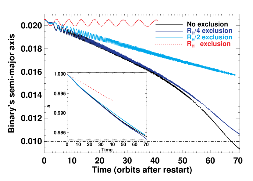
To further illustrate the connection between the hardening of the binary and the flow inside its Hill radius, we performed additional simulations wherein the calculation of the force exerted by the disk on the stars excludes a fraction $f$ of the binary’s Hill radius. Differently said, the binary stars feel the force exerted by all the fluid elements, except those located inside a circle centered on the binary’s center of mass and of radius $fR_{\rm H}$. We took three values for $f$: $1/4$, $1/2$ and $1$. The results of these simulations are displayed in Figure 5. The result with $f=0$, which corresponds to the simulation presented in Figure 4, is overplotted for comparison. The time in $x-$axis is that after the restart (namely, after the first $500$ fixed circular orbits during which the satellite opens a gap). The binary’s hardening rate decreases with increasing $f$. When the torque evaluation discards all of the Hill radius, the binary’s hardening rate is vanishingly small. This result clearly shows that the hardening of the binary is caused by the gas inside its Hill radius. In addition, the very similar results obtained with $f=0$ and $f=1/4$ show that the hardening does not stem from the gas directly surrounding the stars (the two densest points in the top-right panel of Figure 2), which is poorly resolved. The progressive decrease of the hardening rate from $f=1/4$ to $f=1$ confirms that the hardening does arise from the tails lagging the stars.

The inset plot in Figure 5 depicts the time variation of the semi-major axis of the binary’s center of mass obtained with the previous simulations. The migration rates obtained with $f=0$ and $f=1/2$ are in very close agreement, whereas the binary’s hardening rates differ by a factor of $\sim 2$. It suggests that the hardening of the binary has a very limited impact on its migration rate. For $f=1$ (no hardening), the migration rate takes a smaller value, in agreement with the findings with a single-star satellite (Crida et al., 2009). Our results thus show that the hardening rate of the binary is primarily triggered by the disk inside the binary’s Hill radius, whereas its migration rate is controlled by the disk outside of its Hill radius. Our calculations do not suggest there is a significant feedback from one rate on the other. This result does not mean that modelling the global disk structure around the central black hole is unnecessary. Akin to the single satellite case, the flow of gas entering and leaving the Hill radius depends indeed on the interaction of the satellite with the whole disk (e.g., by the capture of fluid elements inside the satellite’s horseshoe region). We finally comment that as the binary hardens, more gas can flow inside the binary’s Hill radius, which can explain the slow increase of the binary’s hardening rates seen in the middle panel of Figure 4.

6.3. Parameter-space study

Figure 6.— Influence of the disk and satellite parameters on the time evolution of the binary’s semi-major axis. In all panels, the horizontal dash-dotted line shows the value of the stars softening length. Top-left: results of simulations with increasing the unperturbed surface density $\Sigma_{0}(a_{0})$ at the binary’s initial location (solid curves). The black solid curve shows the result of the simulation in § 6.2. The black dotted curve shows the result of the same simulation restarted at $280$ orbits (instead of $500$ orbits). Dashed lines show linear fits to the numerical results, assuming the hardening rate $|\dot{a}_{\rm bin}|$ at the restart time scales with $\Sigma_{0}(a_{0})$ (see text). Top-right: results of an additional simulation with a smaller viscosity. Again, dashed lines show linear fits to the numerical results, assuming $|\dot{a}_{\rm bin}|$ scales with $\nu$. Bottom-left: result of a simulation with a slightly smaller disk aspect ratio. Bottom-right: calculation results with different satellite to primary mass ratios.

Figure 7.— Dependence of the binary’s hardening rate with numerics. We show the impact of the grid’s resolution at a fixed softening length (top solid curves), and of the softening length at a fixed grid’s resolution. In the latter case, results are shown with discarding the torque of the fluid elements located inside $1/4$ of the binary’s Hill radius (bottom solid curve), and without such exclusion (dotted curve). The corresponding values of $\varepsilon$ are depicted as horizontal dash-dotted lines.

We have shown in § 6.2 that the interaction between a binary star and the gaseous disk it is embedded in leads to the hardening of the binary as it migrates inward. The hardening timescale is found to be much shorter than the migration timescale. This section is aimed at investigating the dependency of the hardening timescale upon the disk and satellite properties, and upon numerics. A detailed exploration of the parameters space is outside the scope of this paper. Disk and satellite parameters are allowed to vary within a narrow range of values such that the main assumption of our model (the binary opens a gap) is fulfilled.

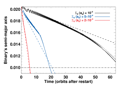
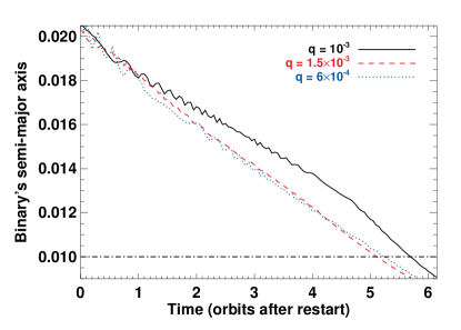
We first consider the impact of the unperturbed surface density at the binary’s location. Two additional simulations were performed with $\Sigma_{0}(a_{0})=5\times 10^{-4}$ and $\Sigma_{0}(a_{0})=2\times 10^{-3}$. The initial Toomre parameter $Q_{0}$ at the binary equals $32$ and $8$, respectively. The result of these simulations, and that of the run of § 6.2, are displayed in the top-left panel of Figure 6 (solid curves). Increasing the unperturbed density results in a faster hardening of the binary. For $Q_{0}(a_{0})=8$, which can be seen as a representative value for our original model in § 2, the binary’s semi-major axis is reduced by a factor of $2$ in only $\sim 5$ orbits. In that case, the mass enclosed in the binary’s Hill radius when it starts to harden is about 50 times smaller than the binary’s mass itself. The dependence of the hardening rate with varying $\Sigma_{0}(a_{0})$ can be interpreted as follows. As the binary is held on a fixed orbit, and because self-gravity is neglected, the fractional change $(\Sigma-\Sigma_{0})/\Sigma_{0}$ of the gas surface density is independent of $\Sigma_{0}$. This is true in particular inside the binary’s Hill radius, which suggests that the net torque exerted by the trailing tails on each star, and therefore the binary’s hardening rate $|\dot{a}_{\rm bin}|$, should scale with $\Sigma_{0}(a_{0})$. The upper dashed curve displays a linear fit to $a_{\rm bin}(t)$ for $\Sigma_{0}(a_{0})=10^{-4}$. The two bottom dashed curves depict previous fit with a slope increased proportionally to the unperturbed density. The good agreement with the calculation results confirms that $|\dot{a}_{\rm bin}|$ is approximately proportional to $\Sigma_{0}(a_{0})$.

We have also checked the dependence of the hardening rate on the restart time of our simulations. Restarting the run of § 6.1 at 280 orbits gives the result overplotted in the top-left panel of Figure 6 as a dotted curve. It is in very close agreement with the calculation result of § 6.2 where the restart time is $500$ orbits, despite the fact the running-time averaged torque has not yet reached a steady-state in either case (see right panel of Figure 3). This agreement is consistent with the fact that the binary’s hardening is driven by the density distribution within its Hill radius, which attains a faster steady-state than the density distribution in the gap. We have obtained the same good agreement with $\Sigma_{0}(a_{0})=2\times 10^{-3}$.

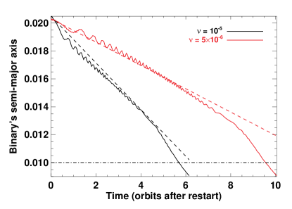
We now assess the impact of the parameters altering the gap properties, taking $\Sigma_{0}(a_{0})=2\times 10^{-3}$ for convenience. The result of calculations with varying the disk’s kinematic viscosity is displayed in the top-right panel of Figure 6 (the run with $\nu=10^{-5}$, which corresponds to $\alpha=4\times 10^{-3}$ at the planet’s location, is the same as in the left panel of this figure). Increasing the viscosity results in a faster hardening. Again, this result can be explained by the fact a larger viscosity induces a larger mass flow in the satellite’s Hill radius, thereby increasing the amplitude of the drag force on each star. As in the top-left panel of Figure 6, the dashed curves highlight that the binary’s hardening rate is proportional to the disk viscosity. We have checked that this result is quantitatively consistent with the density in the binary’s Hill radius scaling proportional to the viscosity. We have also checked that, as expected, the migration rates obtained in these two runs scale with the disk viscosity.

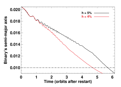
The bottom-left panel of Figure 6 compares the results obtained with a disk aspect ratio $h=5\%$ and $h=4\%$. Our simulations show that the hardening is slightly faster with a smaller disk aspect ratio, the hardening timescales differing by about $20\%$. In the same vein, the bottom-right panel of Figure 6 shows results with different (albeit close) values of the satellite to primary mass ratio, ranging from $q=6\times 10^{-4}$ to $q=1.5\times 10^{-3}$. These simulations have the same $a_{\rm bin,0}$. Our calculation results show that, for the range of values that we considered, $q$ also has little impact on the binary’s hardening rate. We have checked that the density distributions in the binary’s Hill radius show very little dependence with the aforementioned values of $h$ and $q$, which is consistent with our findings. The gap’s depth, however, largely differs between these runs, and so do the migration rates. We point out that in the simulation with $q=6\times 10^{-4}$ and $h=5\%$, the binary experiences inward runaway migration, in agreement with Masset & Papaloizou (2003).

Figure 8.— Left: surface density contour at $500$ orbits of the disk perturbed by a retrograde binary held on a fixed circular orbit. Right: close-up of the density distribution around the retrograde binary. As in Figure 2, the dashed circle shows the binary’s Hill radius, and part of the computational grid is overplotted in the bottom-left part of the panel.

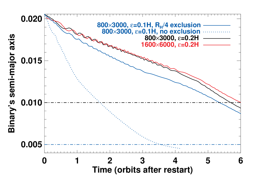
We now discuss the dependence of our findings on the resolution of our calculations. As already stressed in § 4.2, resolution is controlled by the softening length $\varepsilon$ of the stars potential, and by the grid’s resolution. We study in this paragraph the impact of both parameters. Two additional calculations were performed with $\Sigma_{0}(a_{0})=2\times 10^{-3}$: one with doubling the number of grid cells along each direction, and one at our standard resolution but with $\varepsilon=0.1H$ (that is, half our standard softening length). Results are depicted in Figure 7. For our fiducial value of $\varepsilon$, increasing the grid’s resolution is found to have no impact on the hardening rate. Decreasing the softening length at same resolution yields however a dramatic raise of the hardening rate (dotted curve). While the density inside the binary’s Hill radius, in particular at the location of the tails, takes similar values for both values of $\varepsilon$, the gas density at the immediate vicinity of the stars is increased by about one order of magnitude for $\varepsilon=0.1H$. It clearly suggests that the large mass accumulation around the stars is severely under-resolved, in contrast to the results presented with our fiducial softening length, and that the resulting increase of the hardening rate is a numerical artifact triggered by a lack of resolution. To illustrate this statement, we performed an additional simulation at $\varepsilon=0.1H$, wherein the binary’s time-evolution discards the torque exerted by the fluid elements located inside a circle of radius $R_{\rm H}/4$ centered on the binary’s center of mass. As already stated in § 6.2, such radius is meant to discard the torque due to the mass accumulation around the stars, with very small impact on the torque exerted by the tails (see Figure 5). The result of this simulation is overplotted in the bottom-right panel of Figure 7, and shows a good agreement with the result at larger softening.

6.4. Case of a retrograde binary

Figure 9.— Orbital evolution of retrograde and prograde binaries. Hardening rates and migration rates are compared in the left and right panels, respectively. The horizontal dash-dotted line in the left panel shows the value of the stars softening length.

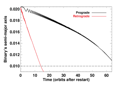
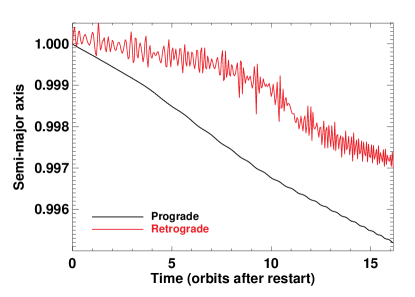
The calculation results presented in previous sections assume a prograde binary, with the angular momentum vectors of the disk and of the binary being aligned. It is possible that this relative inclination takes very different values when the binary forms in the disk, or after it formed, through dynamical interactions with other stars or more massive objects. Another possibility is that the binary did not form in the disk, and was captured. One expects that the gaseous disk dampens the relative inclination on a rather short timescale. Since our calculation results suggest that the binary’s hardening may also occur on short timescales, it is relevant to investigate the general case of a random disk–binary relative inclination. We limit ourselves to the case of a retrograde binary. The binary’s center of mass still has a prograde motion around the black hole.

We performed one simulation with a retrograde binary, using the procedure and parameters described at the beginning of § 6. Akin to the prograde case shown in Figure 2, the disk’s surface density obtained at $500$ orbits with the retrograde binary is displayed in the left panel of Figure 8 (note that the color scales differ in both figures). We observe that the gap is less deep in the retrograde case. We have measured that the azimuthally-averaged density in the gap is a factor of $2$ to $3$ larger compared to the prograde case. The right panel of Figure 8 shows a close-up of the disk density around the retrograde binary, whose Hill radius is drawn as a dashed circle. In this panel, the stars rotate clockwise. A comparison with the top-right panel of Figure 2 reveals that the mass enclosed in the Hill radius is about one order of magnitude larger in the retrograde case. We attribute these differences to a larger velocity difference in the retrograde case between the stars and the fluid elements approaching the stars on horseshoe trajectories. Those fluid elements are therefore less deflected as they get closer to the stars, and they can enter the binary’s Hill radius more easily.

Similarly as in the prograde case, overdense spiral tails lag the stars. The tails should therefore extract angular momentum from the retrograde binary, which we expect to harden with time, just like the prograde binary. This is confirmed in the left panel of Figure 9, where the time evolution of the binary’s semi-major axis is displayed for both the prograde and the retrograde binaries. The horizontal dash-dotted curve depicts the stars softening length. The hardening timescale is a factor of $5$ to $10$ shorter than in the prograde case, which can be attributed to the relative difference of the density in the Hill radius between the retrograde and prograde binaries. The right panel of Figure 9 compares the semi-major axis of the binary’s center of mass in both cases. The inward migration of the retrograde binary is much slower on average, which is most presumably due to a shallower gap profile.

7. Back to the original problem

Figure 10.— Surface density contour at $300$ orbits obtained with the parameters of the original problem ($q=10^{-5}$, $h=1\%$, and $\alpha=10^{-3}$). The binary’s Hill radius is shown as a dashed circle, and part of the computational grid is overplotted in the bottom-left part of the panel.

Figure 11.— Time evolution of the binary’s semi-major axis obtained with the disk and satellite parameters of the original problem (solid curve), and of the rescaled problem with same initial density (dashed curve). For comparison purposes, the ratio $a_{\rm bin}/a_{\rm bin,0}$ is displayed in y-axis. The time in x-axis is in units of the orbital period of the binary’s center of mass around the central black hole. The horizontal dash-dotted line depicts the ratio $\varepsilon/a_{\rm bin,0}$, which is identical in both simulations.

Our original problem is to investigate the tidal interaction of a massive ($q=10^{-5}$) binary star and its natal thin ($h\sim 1\%$) gaseous disk. We have justified in § 5 that, for a single-star satellite, one can instead tackle a less computationally demanding rescaled problem, where the properties of the disk–satellite interaction (gap properties, amount of gas in the satellite’s Hill radius, value of the specific torque on the satellite) remain essentially unchanged. The calculation results in § 6 have been obtained with the parameters of the rescaled problem: $q=10^{-3}$, $h=5\%$ and $\alpha=4\times 10^{-3}$. We have shown that, in addition to migrating inward, the binary system hardens, due to the net drag force exerted by each companion’s wake inside the binary’s Hill radius. Our results indicate that the hardening timescale is inversely proportional to the unperturbed density in the binary’s Hill radius, and that it is shorter than the migration timescale by typically one to two orders of magnitude.

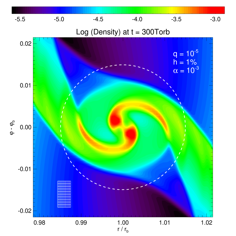
We have shown in § 6.1 that the gap properties and the specific torque obtained with single and binary satellites are in good agreement. This agreement implies that the steady-state migration rate of a binary satellite should be similar in the original and rescaled problems, as in the case of a single satellite detailed in § 5. However, it is not clear whether the hardening rate remains unchanged when applying the rescaling method. To check this, we performed a simulation with the parameters of the original problem. The unperturbed surface density at the binary’s location is $10^{-4}$, as in the simulation of § 6.2. This sets the initial Toomre parameter at the binary’s location to $\approx 32$. For comparison purposes, we kept the same ratios $a_{\rm bin}/R_{\rm H}$ and $a_{\rm bin}/\varepsilon$, which leads to $a_{\rm bin}\approx 4\times 10^{-3}a$ and $\varepsilon\approx 2\times 10^{-3}a$. The satellite’s Hill radius is resolved by about $50$ cells along the radial direction, and $24$ along the azimuthal direction (to be compared with $50$ and $33$, respectively, in the simulations of § 6). A close-up of the gas surface density around the binary star is displayed at $300$ orbits in Figure 10. It is very similar to the density obtained at $500$ orbits in the rescaled problem (top-right panel of Figure 2). This similitude is due to (i) the use of (almost) the same dimensionless parameters in the gap-opening criterion, and to (ii) the fact the density in the satellite’s Hill radius reaches a faster steady-state than the density in the gap. We notice that the density at each perturber’s wake is a factor of $\approx 2$ larger in the original problem.

The time evolution of the binary’s semi-major axis obtained with previous simulation restarted at $300$ orbits is depicted in Figure 11 (solid curve). To compare with the result of the rescaled problem (dashed curve), the ratio $a_{\rm bin}/a_{\rm bin,0}$ is displayed in y-axis. The binary’s semi-major axis in the original problem decreases by a factor of two in about $8$ to $10$ orbits, or in about $130$ orbits of the stars around their center of mass. This corresponds to $\sim 1.5\times 10^{4}$ yrs at $0.1$ pc in the Galactic center case. The slowing down of the binary’s hardening rate after $\approx 8$ orbits is most presumably due to the fact that $a_{\rm bin}$ becomes comparable to the softening length of the stars potential. The hardening timescale in the original problem is shorter than that of the equivalent rescaled problem by a factor of $8$ to $10$. This timescale difference can be qualitatively interpreted as due to different mass ratios of the binary and of the gas in the binary’s Hill radius. Between the original and rescaled problems, the binary’s mass is increased by a factor of $100$, whereas the mass inside the binary’s Hill radius in increased by a factor of $\sim 20$ (ratio of the Hill radii squared). This simple argument suggests a hardening timescale $\sim 5$ times larger in the rescaled problem, which is in correct agreement with our findings.

Some further insight can be gained by using the analytic prediction of Stahler (2010). Through a linear analysis of the Euler equations, he derived the timescale for the orbital decay of a low-mass binary embedded in a three-dimensional static medium of gas. Applying his equation 56-a to our disk model (writing the sound speed $c_{\rm s}=H\Omega$, the 3D unperturbed gas density $\rho_{0}\approx\Sigma_{0}/2H$, noticing from our simulations that a typical density in the binary’s Hill radius is the unperturbed density at the binary’s initial location), the extrapolated hardening timescale $\tau_{\rm hard}$ may be estimated as

$$\tau_{\rm hard}\sim 0.6\left(\frac{Q}{h}\right)\left(\frac{q}{h^{3}}\right)^{-2}\left(\frac{a_{\rm bin}}{a}\right)T_{\rm orb},$$ (11)

where $T_{\rm orb}$ is the orbital period of the binary’s center of mass around the central black hole. Since our original and rescaled simulations have the same $Q/h$ (that is, the same unperturbed density at the binary’s location), Eq. (11) predicts that the hardening timescale in the original problem should be a factor of $8$ shorter than in the rescaled problem, which is in good agreement with our results of simulations. For convenience, Eq. (11) can be recast as

$$\left.\tau_{\rm hard}\right. \sim 900\;{\rm yr}\times\left(\frac{T}{2000\;{\rm K}}\right)^{3}\left(\frac{\Sigma}{10^{2}\;{\rm g\;cm}^{-2}}\right)^{-1}$$ (12)

$$\times \left(\frac{M_{\rm smbh}}{3\times 10^{6}\;M_{\odot}}\right)^{-1/2}\left(\frac{M_{\rm bin}}{2\;M_{\odot}}\right)^{-2}$$

$$\times \left(\frac{a}{\rm 0.1\;pc}\right)^{3/2}\left(\frac{a_{\rm bin}}{\rm 50\;AU}\right),$$

where $M_{\rm bin}$ denotes the binary’s mass, and where $T$ and $\Sigma$ are the unperturbed gas temperature and surface density at the binary’s location. In Eq. (12), we have assumed a mean molecular weight $\mu=2.4$, and an adiabatic index $\gamma=5/3$.

With the parameters of the original problem, Eq. (11) predicts a hardening timescale $\lesssim 0.1$ orbit, that is about two orders of magnitude shorter than in our simulation. We comment that, while Eq. (11) may capture the right functional dependence of the hardening timescale with the disk and satellite parameters in our problem, a quantitative comparison with our results of simulations seems inappropriate, since the key assumption in Stahler (2010)’s analysis (each perturber’s wake induces a small perturbation of the background gas density, which can be described with a linear analysis) is clearly not satisfied in our simulations (see e.g., Figure 10). Another source of discrepancy may also be triggered by the time-varying velocity difference in our simulations between the binary and the gas inside the Hill radius.

8. Discussion

8.1. Motivation

The primary astronomical motivation of the investigation presented here is to explore the origin of the “S-stars”, a population of relatively massive stars in the inner $0.05$ pc of the Galactic center. The S-stars could be related to those in coplanar orbits just outside this inner region. It is natural to assume that these disk-stars may have either coherently formed in (Levin, 2007) or rapidly accreted gas (Artymowicz et al., 1993) from a common gaseous disk.

Most of the S-stars have large eccentricities and random inclinations (e.g., Lu et al., 2009). In contrast, the nearby disk-stars have smaller eccentricities and their velocity dispersion is an order of magnitude smaller than the local Keplerian speed. One potential explanation for their large eccentricities and random inclinations is that the S-stars originated from the tidal disruption of binary systems that were scattered to the proximity of the central supermassive black hole on nearly parabolic orbits (Gould & Quillen, 2003). This scenario would also account for the observed hypervelocity stars in the Galactic halo, provided some of the scattered binaries have very close separation (Hills, 1988; Yu & Tremaine, 2003; Gualandris et al., 2005; Lu et al., 2010; Zhang et al., 2010), typically within a few solar radii.

In this paper, we consider a unified scenario for the young, massive stars near the Galactic center (both disk- and S-stars) and high-velocity stars in the Galactic halo. We assume their progenitors were binary stars that formed at large distance (a fraction of a pc) from the SMBH, in a gaseous disk that we expect existed in the Galactic center in the past. In principle, similar to the solar neighborhood, binary systems could be as common as single stars and have a logarithmic period distribution (Duquennoy & Mayor, 1991). Around the Galactic center, however, tidal interaction between binary systems and their natal disk induces angular-momentum exchange between them. The main outstanding issue is whether these binaries’ center of mass would migrate (presumably inward) extensively before they harden substantially.

8.2. Model

We have investigated the tidal interaction of a binary star and its natal gaseous disk by means of two-dimensional hydrodynamical simulations. For illustration purpose, we have considered a fiducial binary system, comprising two equal-mass ($15\;M_{\odot}$) stars embedded in a thin ($h=1\%$), moderately turbulent ($\alpha=10^{-3}$) gaseous disk around a $3\times 10^{6}\;M_{\odot}$ SMBH. These initial and boundary conditions are such that the binary opens a deep gap around its orbit, and is thus subject to type II migration. We have shown in § 5 that this gap-opening process has helped us transform our original problem into an equivalent, less computationally demanding rescaled problem. We have presented results of calculations of the rescaled problem in § 6, and of the original problem in § 7.

We have made a number of simplifying assumptions in the models presented here (see § 2). We have neglected the process of gas accretion onto the stars, assuming the latter already reached their final mass at the beginning of the simulations. We have also assumed throughout this paper that the binary stars formed in a circular orbit, while the fragmentation of an eccentric gaseous disk would put them in initially eccentric orbits (e.g., Nayakshin et al., 2007; Alexander et al., 2008b). While we expect many stars to form at the same time in a fragmenting gas disk, we have considered the evolution of a single isolated satellite (one binary star). The presence of many embedded stars, each propagating density waves, and opening a gap for the most massive ones, would dramatically impact the gas disk structure. The properties of disk–satellite interactions, and the resulting migration timescale, could be very different from those of a single isolated satellite. The interaction between different satellites could excite their orbital eccentricity and alter their migration rate, leading for example to captures into mean-motion resonance or scattering events (e.g., Cresswell & Nelson, 2008; Marzari et al., 2010). Also, encounters with other single stars may help to further harden binary stars, especially at short separations from the supermassive black hole (e.g., Perets, 2009). We defer this interesting regime for future study.

The properties of the gaseous disk after star formation are largely uncertain and poorly constrained. We have grossly simplified the evolution of the underlying gaseous disk, in particular by neglecting the depletion of the gaseous disk, and the increase of its temperature under star formation. Local heating of the gas disk by the intrinsic luminosity of the embedded stars could modify the mass flow inside the binary’s Hill radius, and therefore the binary’s hardening rate. The progressive depletion of the gas disk also implies a finite timescale over which disk–satellite interactions are effective. In the context of Sgr A*, we mention the work of Nayakshin et al. (2007), who performed hydrodynamical simulations of star formation in a gaseous disk around the central SMBH, including a crude treatment of thermal accretion feedback (a fraction of the star accretion luminosity is converted into disk heating). Their simulations indicate that the disk’s mass may be reduced by a factor of two in at most $10^{5}$ yrs (about $60$ orbital periods at $0.1$ pc). It is much shorter than the timescale for gas accretion onto Sgr A* through turbulent transport of angular momentum (Nayakshin & Cuadra, 2005). It is also much shorter than the expected timescales for type I and type II migration, but not necessarily short compared to the timescale for type III migration (see § 3). Still, this potentially short lifetime of the gas disk is a challenge for migration driven by disk torques. However, it may not be a stringent constraint on the hardening of massive binary stars driven by the gas disk, which we find to occur on a timescale comparable to, or shorter than the aforementioned disk lifetime, as is recalled in § 8.3.

8.3. Summary of our results

Our main result is that the binary gets harder as it migrates toward the central black hole. The hardening timescale is much shorter than the migration timescale, which is very similar to that of a single satellite of the same mass. The binary’s hardening rate is essentially determined by the gas density inside the binary’s Hill radius. In that region, overdense spiral tails lag the stars, exerting a torque on them and hardening their orbit. The gas density at the tails location, and therefore the hardening rate, scale with the viscosity and with the unperturbed surface density of gas at the binary’s location (i.e. prior to gap formation). Assuming that at this location, the $\alpha$ viscous parameter is $\sim 10^{-3}$, and the initial Toomre parameter (before gap formation) is $\approx 32$, we find that the separation between the stars is reduced by a factor of $2$ in about $10$ orbits of the binary around the central black hole (see § 7). Scaled to the Galactic center case, that is in only $\sim 2\times 10^{4}$ yrs at $0.1$ pc, which is several orders of magnitude shorter than the expected migration timescale. A larger initial surface density would yield an even shorter hardening timescale. In the rest of this section, we discuss the evolution of low-mass binary stars (namely, what could have happened prior to our initial condition), and the subsequent evolution of massive binary stars (that is, what could occur after the end of our simulations).

8.4. Hardening of low-mass binary stars

It is likely that disk–satellite interactions significantly impact the binary’s semi-major axis from the early stages of the binary’s formation, well before the binary has attained its asymptotic mass and potentially opened a gap around its orbit. In that case, the wake of each star would induce a low-amplitude density perturbation in the background gas surrounding the stars. This situation would resemble the one investigated by Stahler (2010). The hardening timescale extrapolated from his analytic study to our disk model is given at Eqs. (11) and (12). Assuming the unperturbed gas disk has $Q\sim 32$, $h\sim 1\%$ (that is, $\Sigma\sim 6$ g cm^-2 and $T\sim 2000$ K at the binary’s location), and taking a low-mass binary ($1\;M_{\odot}$ stars, so that $q/h^{3}\lesssim 1$ and the linearization assumption should be valid) with $a_{\rm bin}\sim 0.3R_{\rm H}$ (as in our simulations; here it corresponds to $a_{\rm bin}\sim 40$ AU), Eqs. (11) or (12) give $\tau_{\rm hard}\approx 1.2\times 10^{4}$ yr at $a=0.1$ pc. This timescale is similar to the one obtained in our 2D simulations, but note the strong dependence of $\tau_{\rm hard}$ with both $q$ and $h$. The dynamical evolution of a low-mass binary subject to hardening during its type I migration deserves follow-up investigation with self-consistent high-resolution 3D simulations.

8.5. Subsequent binary evolution

The results in § 6 and 7 provide the initial hardening rate for massive (gap-opening) binary stars with separation close to their Hill radius. We underscore that our simulations cannot, and do not address the final outcome of the binary’s hardening, i.e. whether binary stars will ultimately coalesce, form a very hard binary, or become disrupted. We can only extrapolate some possible implications of the binary’s fast hardening in our model.

8.5.1 Opening of a cavity

As a massive binary star shrinks, residual gas is preserved in a viscous disk between its orbit and its Hill radius. Tidal interaction between the binary and the disk around it leads to angular momentum transfer from the stars’ orbits to the inner disk region. Similarly, angular momentum is removed from the outer region of the disk by the SMBH’s tidal torque. The binary’s hardening rate is determined by an equilibrium (outward) flux of angular momentum. Our results suggest this rate may be maintained at a fairly large value at least until the binary separation is less than about one sixth of its Hill radius. Our results also suggest that the disk interior to the binary stars’ orbit should be cleared by their tidal torque such that this region is expected to evolve into a cavity. In that case, the inside of the binary’s Hill radius would comprise the binary star, the cavity where the binary now evolves in, and the surrounding gas disk referred to as the circumbinary disk (the cavity should not be confused with the gap that the satellite opens or has opened in the global disk structure around the SMBH). It remains however to be clarified how the timescale associated with gas removal from inside the binary’s orbit compares with the binary’s shrinking timescale before a cavity is opened. In the next paper of this series, we will present high-resolution hydrodynamical simulations to make this comparison. If the binary manages to maintain a cavity, the tidal interaction between the binary and the circumbinary disk would keep on hardening the binary, at slower rates than the initial pace we found here. Otherwise, the binary could keep on hardening until it coalesces. It is thus possible that some of the massive stars near the Galactic center result from coalescences of binary-star systems, which might contribute to account for the top-heavy initial mass function observed in the two stellar disk structures in the Galactic center (Bartko et al., 2010). However, such stars would still be embedded in a gaseous disk around the SMBH, and therefore in nearly-circular orbits. Resonant relaxation (e.g., Rauch & Tremaine, 1996; Perets et al., 2009), the presence of short-lived massive stars or of intermediate mass black holes (e.g., Yu et al., 2007), or an initially-eccentric gaseous disk (e.g., Cuadra et al., 2008) could explain their observed current eccentricities.

The hardening process with a cavity inside the binary’s orbit is very similar to type II migration: the tidal torque of the binary competes with the viscous torque from the circumbinary disk (see e.g., Pringle, 1991; Artymowicz et al., 1991; Syer & Clarke, 1995; Ivanov et al., 1999). This problem shares a number of analogies with the hardening of binary black-holes surrounded by a circumbinary disk (e.g., Cuadra et al., 2009, where the transport of angular momentum is due to the disk self-gravity). We take the separation $r_{\rm o}$ between the binary’s center of mass, and the location in the circumbinary disk where most of the binary’s angular momentum is deposited (that is, near the inner edge of the circumbinary disk), equal to $a_{\rm bin}$. Further assuming that the gas density $\Sigma$ at that location is still as large as $\sim 10^{2}\;{\rm g\;cm}^{-2}$, the ratio $4\pi\Sigma a^{2}_{\rm bin}/M_{\rm bin}\sim 5\times 10^{-2}\ll 1$ for a $M_{\rm bin}=30\;M_{\odot}$ binary with separation $a_{\rm bin}\sim 100\;{\rm AU}$. The asymptotic hardening timescale $\tau_{\rm hard,as}$ of the binary thus corresponds to the timescale for satellite-dominated type II migration (see § 3.2). Using Eq. (7), we have

$$\tau_{\rm hard,as}\sim\frac{M_{\rm bin}}{6\pi\nu\Sigma},$$ (13)

where $\Sigma$ and $\nu$ denote the surface density and kinematic viscosity at $r_{\rm o}$. Further writing $\nu=\alpha c_{\rm s}^{2}\Omega^{-1}$, with $c_{\rm s}$ and $\Omega$ the sound speed and angular velocity of the circumbinary disk, we obtain

$$\left.\tau_{\rm hard,as}\right. \sim 9\;{\rm Myr}\times\left(\frac{\alpha}{10^{-3}}\right)^{-1}\left(\frac{T}{2000\;{\rm K}}\right)^{-1}\left(\frac{M_{\rm bin}}{30\;M_{\odot}}\right)^{3/2}$$ (14)

$$\times \left(\frac{\Sigma}{10^{2}\;{\rm g\;cm}^{-2}}\right)^{-1}\left(\frac{a_{\rm bin}}{\rm 100\;AU}\right)^{-3/2},$$

where we have assumed a mean molecular weight $\mu=2.4$, and an adiabatic index $\gamma=5/3$. The unknown values of $\alpha$, $T$ and $\Sigma$ near the inner edge of the circumbinary disk make the value of $\tau_{\rm hard,as}$ largely uncertain. In order to compare with the hardening timescale inferred from our simulations, we arbitrarily assume that $\alpha$, $\Sigma$ and $T$ take similar values as in our physical model in § 2, which however describes the properties of the star-forming gas disk around the SMBH. This choice is also motivated by the simplifying assumption that the circumbinary disk is in a quasi-steady state. The quantity $\nu\Sigma$ in Eq. (13) then becomes independent of the separation from the binary’s center of mass, and it may be evaluated near the outer edge of the circumbinary disk (where $\alpha$, $c_{\rm s}$ and $\Omega$ should not dramatically differ from their value in the star-forming disk about the central SMBH, at the binary’s location). Thus taking $T\sim 2000$ K, $\Sigma\sim 10\;{\rm g\;cm}^{-2}$, $\alpha\sim 10^{-3}$, $M_{\rm bin}=30M_{\odot}$, and $a_{\rm bin}\sim 100$ AU, we get $\tau_{\rm hard,as}\approx 90$ Myr. This timescale is, as expected, much longer than the hardening timescale with no cavity inside of the binary’s orbit. Even with considering a more conventional larger $\alpha$, smaller values of $\Sigma$ due to the progressive disk depletion should maintain $\tau_{\rm hard,as}$ to a value that presumably exceeds a few Myr. This is comparable to, if not larger than the lifetime of the most massive stars near the Galactic center, indicating that stellar evolution should be taken into account (see § 8.5.2).

We finally point out that there is no indication in Eq. (14) as to why the binary’s shrinkage should stop. We mention the possibility that the gas in the circumbinary disk may be progressively stripped due to stellar winds, or to multiple close encounters with other stars, as was observed by Nayakshin et al. (2007). If the shrinkage is sufficiently efficient to decrease the binary’s separation to a few stellar radii, mass transfer due to Roche lobe overflow will control the binary’s subsequent evolution. If the donor star expands faster than its Roche lobe, or shrinks less rapidly than its Roche lobe for a prolonged time, mass transfer will be unstable, which may lead to a common-envelope phase and, perhaps, a merger.

8.5.2 Including stellar evolution: the explosive disruption scenario

Figure 12.— Outcome of the supernova disruption of a binary star orbiting a $M_{\rm smbh}=3.5\times 10^{6}M_{\odot}$ black hole. Before disruption, the primary’s mass is $M_{1}=20M_{\odot}$, and the secondary’s mass is either $M_{2}=15M_{\odot}$ (left panel), or $M_{2}=4M_{\odot}$ (middle and right panels). We assume that the primary loses enough mass so that the binary becomes disrupted. Before disruption, the internal and orbital angular momentum vectors of the binary are taken aligned. We assess in this figure the properties of the two-body orbit of the secondary with the black hole (see text for details). In all contour plots, the binary’s internal separation $a_{\rm bin}$ is depicted in x-axis, and the separation $a$ between the black hole and the binary’s center of mass is in y-axis. The left panel shows the mean eccentricity of the bound secondaries. The middle panel displays the fraction of escapers, namely the secondaries that become unbound to the black hole. The escapers’ mean velocity at infinity is shown in the right panel.

Including stellar evolution, and the likely possibility of unequal-mass binaries, we now consider the outcome of binaries that have reached small enough separations. If the more massive (primary) star evolves into a red giant with a radius comparable to the binary separation, both stars undergo common envelope evolution. The engulfed binary hardens again due to the drag force exerted by the gas on each star. The energy lost by the binary system leads to the expansion of the gas envelope. This is reminiscent of the opening of a cavity by a binary embedded in a gaseous disk, discussed in § 8.5.1. The successful ejection of the common envelope, and therefore the binary’s survival, depend on the binary separation before the common envelope stage, and on the primary’s mass (see e.g., the review by Taam & Sandquist, 2000). If the binary survives the common envelope evolution (i.e. if it does not coalesce), it then comprises an Helium-rich star and an OB-star companion.

Many stars near the Galactic center lose mass through Wolf-Rayet winds. With a substantial mass loss, the primary may evolve into Wolf-Rayet or blue supergiant stars. Mass loss typically results in increasing the binary separation, but in our scenario this trend is offset by the disk presence. In this case, the binary separation can be reduced to several solar radii, and may avoid another common envelope evolution if the primary explodes as a supernova. The outcome of the primary’s explosion depends on the fraction of the primary’s mass that is ejected. If they explode, typical blue supergiants (with a mass $\sim 10-20\;M{{}_{\odot}}$) may lose most of their residual envelope during their supernova explosion. If the mass lost to the supernova ejecta is more than half of the binary’s mass before explosion, the compact binary would become unbound (Hills, 1983), and the secondary could attain a recoil velocity that is a significant fraction of the primary’s surface escape velocity.

What velocities can we expect in the supernova disruption scenario? The simplest approach is to look at the properties of the two-body orbit of the secondary about the central black hole. Before disruption, we assume that the binary’s center of mass is on a circular orbit with semi-major axis $a$, and the binary’s internal separation is $a_{\rm bin}$ (we neglect the binary’s internal eccentricity $e_{\rm bin}$ for simplicity). We also assume that the primary’s supernova has no impact on the secondary: the mass and velocity of the secondary before and after disruption are taken the same. We will come back to this assumption below. In the frame centered on the black hole, the velocity of the secondary is the sum of the velocity of the binary’s center of mass about the black hole (${\bf v}_{\rm smbh}$), and of the velocity of the secondary about the binary’s center of mass (${\bf v}_{\rm bin}$). The angle $\theta$ between both velocity vectors is a random variable distributed uniformly between $0$ and $2\pi$, since in our model both velocities are coplanar. Their amplitude is given by

$$v_{\rm smbh}\sim 390\;{\rm km\;s^{-1}}\times\left(\frac{M_{\rm smbh}}{3.5\times 10^{6}\;M_{\odot}}\right)^{1/2}\left(\frac{a}{0.1\;{\rm pc}}\right)^{-1/2},$$ (15)

and

$$v_{\rm bin}\sim 133\;{\rm km\;s^{-1}}\times\left(\frac{M_{1}}{M_{\rm bin}}\right)\left(\frac{M_{\rm bin}}{20\;M_{\odot}}\right)^{1/2}\left(\frac{a_{\rm bin}}{1\;{\rm AU}}\right)^{-1/2},$$ (16)

respectively. In Eq. (16), $M_{1}$ and $M_{2}$ denote the mass of the primary and of the secondary, and $M_{\rm bin}=M_{1}+M_{2}$ is the binary’s mass. In the following, we take $M_{\rm smbh}=3.5\times 10^{6}\;M_{\odot}$, and $M_{1}=20\;M_{\odot}$.

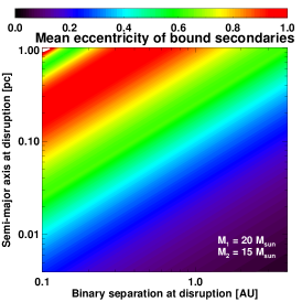
We first consider the case where $M_{2}=15\;M_{\odot}$, a mass similar to that of the S-stars. We vary $a$ from $4\times 10^{-3}$ pc to $1$ pc, and $a_{\rm bin}$ from $0.1$ AU to $4$ AU (both with a logarithmic spacing). The minimum value of $a_{\rm bin}$ is approximately the sum of the two stars radii. Its maximum value is set as about half the smallest Hill radius of our binaries sample. This choice ensures that, before the primary goes supernova, all binaries are bound with modest internal eccentricity. The left panel of Figure 12 shows a contour plot of the mean eccentricity of the secondaries that remain bound to the central object, as a function of $a_{\rm bin}$ (x-axis) and $a$ (y-axis). The average is done over the different values of the angle $\theta$. Large eccentricities, compatible with those of the S-stars, can be obtained with the supernova disruption scenario. We point out that, for sufficiently large $a$ (at a given $a_{\rm bin}$), the mean eccentricity of the bound secondaries decreases, with a local minimum of $\sim 0.6$, and increases again. The presence of this local minimum is due to secondaries put on retrograde, close to circular orbits about the black hole. It is straightforward to show that the minimum’s location satisfies $v_{\rm bin}=2v_{\rm smbh}$, which can be recast as $a\sim 0.6\;{\rm pc}\times(a_{\rm bin}/0.1\;{\rm AU})$ for our set of parameters.

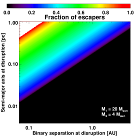
We next consider the case where $M_{2}=4\;M_{\odot}$, a mass similar to that of the hypervelocity stars, and we now vary $a_{\rm bin}$ from $0.07$ AU to $4$ AU. The middle panel of Figure 12 shows the fraction of escapers, these secondaries that are energetic enough to become unbound to the black hole. The fraction of escapers increases with increasing $a$ and decreasing $a_{\rm bin}$, as expected. For maximally hard binaries, the fraction becomes unity for $a\gtrsim 0.4$ pc.

The escapers’ mean velocity at infinity, measured in the frame centered on the SMBH, is shown in the right panel of Figure 12. The large velocities that we obtain suggest that the most energetic escapers could account for some of the Runaway Galactic OB-stars, as originally proposed by Blaauw (1961), or for some of the hypervelocity stars in the Galactic halo. The latter have typical Galactic rest-frame velocities between $400$ and $700\;{\rm km\;s}^{-1}$ (e.g., Brown et al., 2006). Our results indicate that the ejection of secondaries that may still be going faster than $\sim 400$ km s^-1 in the Galactic halo is possible. It however requires binaries that are nearly maximally hard, and primaries that are sufficiently massive (the maximum escapers velocity approximately scales proportional to $\sqrt{M_{1}}$; a primary’s mass before explosion of $\sim 10M_{\odot}$ would yield a maximum escaper’s velocity $\sim 330$ km s^-1).

The suggestion that the hypervelocity stars could originate from the supernova disruption of binaries close to the SMBH is in apparent contradiction with the results of Gualandris et al. (2005), who performed population synthesis studies and found that no binary can produce a hypervelocity star by itself. However, in our scenario, binaries can be kept at very short internal separations due to the action of the gaseous disk. In contrast, standard population synthesis studies do not model the angular momentum loss of binaries in presence of a background disk, and thus produce few very hard binaries. We stress that our study mentions the possibility, but does not estimate the probability to get escapers with velocities comparable to those of the runaway and hypervelocity stars through supernova-disrupted binaries. We finally comment that the distribution of the hypervelocity stars on two thin disks (Lu et al., 2010; Zhang et al., 2010) may be accounted for by both the tidal and the supernova disruption scenarios. In both cases, we need compact binaries originating from two disks near the Galactic center. While the tidal disruption mechanism requires binaries on highly elliptical orbits, the supernova disruption mechanism requires binaries with internal and orbital angular momentum vectors that are nearly aligned.

Only mean quantities are displayed in Figure 12. To give an idea of their standard deviations, we show in Figure 13 the mean and standard deviation of (i) the eccentricity of the bound secondaries (black cross symbols, see left axis), and of (ii) the escapers velocity at infinity (red filled circles, right axis) resulting from nearly maximally hard supernova-disrupted binaries.

Figure 13.— Eccentricity of the bound secondaries (black cross symbols, left axis), and escapers’ velocity at infinity (red filled circles, right axis) resulting from the supernova disruption of nearly maximally hard binaries with aligned internal and orbital angular momentum vectors. Error bars indicate the standard deviation of each quantity.

Figure 14.— Eccentricity (mean and standard deviation shown as error bars, left axis) and inclination (standard deviation, right axis) of the bound secondaries resulting from the supernova disruption of nearly maximally hard binaries with misaligned internal and orbital angular momentum vectors. Two cases are contemplated: one for which the internal angular momentum vector of the binary before disruption points towards the black hole (black cross and square symbols), and one where it is parallel to ${\rm v}_{\rm smbh}$ (blue filled circles and star symbols).

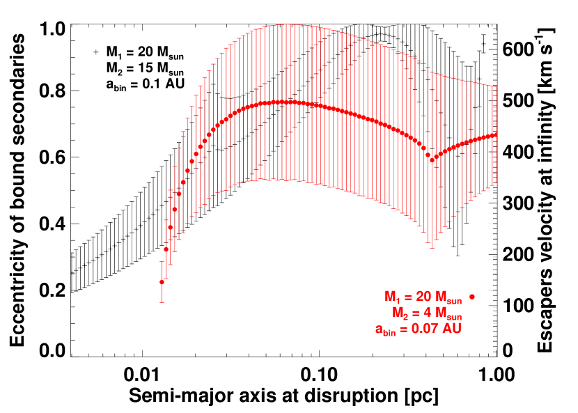
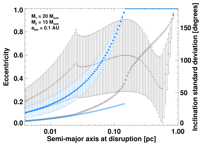
The results shown in Figures 12 and 13 assume that the internal and orbital angular momentum vectors of the binary before disruption are aligned, resulting in a change of the secondaries’ eccentricity, but not of their inclination. Our model assumes that binaries are formed and stay in the same plane as that of the gas disk. While a more general scenario, including possible misalignments and their distribution, is out of this paper’s scope, we briefly underscore the possibility to get secondaries with large inclinations through the supernova disruption scenario. This statement is illustrated in Figure 14, where we display the eccentricity (mean, and standard deviation depicted as error bars), and standard deviation of the inclination of bound secondaries arising from the disruption of nearly maximally hard binaries at different separations from the SMBH ($M_{1}=20M_{\odot},M_{2}=15M_{\odot}$ and $a_{\rm bin}=0.1$ AU). Only two extreme cases are shown, one where the internal angular momentum vector of the binary initially points towards the SMBH (black cross and square symbols), and one where it is parallel to ${\bf v}_{\rm smbh}$ (blue filled circles and star symbols). Our results show that it is possible to obtain secondaries with large inclinations for a broad range of eccentricities (including large ones) through the supernova disruption of very hard, circular binaries. In contrast, the tidal disruption of such binaries can only lead to stars with small inclinations, since the ratio of the binary’s orbital and internal velocities $\sim(M_{\rm smbh}/M_{\rm bin})^{1/3}\gg 1$. A statistical investigation aimed at comparing the outcome of the supernova disruption scenario with the orbital properties of the known S-stars will be presented elsewhere.

We stress that the above results assume a very simple disruption model. In particular, we have discarded the impact velocity imparted by the ejected shell of the primary. Its expression is given by Tauris & Takens (1998). Still assuming for simplicity that the secondary’s mass is not altered by the supernova’s blast wave, the impact velocity $v_{\rm imp}$ can be estimated as

$$v_{\rm imp}\sim v_{\rm sh}\times\left(\frac{R_{2}}{2a_{\rm bin}}\right)^{2}\left(\frac{M_{\rm sh}}{M_{2}}\right),$$ (17)

where $M_{\rm sh}$ and $v_{\rm sh}$ denote the mass and ejection speed of the ejected shell. Taking $v_{\rm sh}\sim 10^{4}$ km s^-1 (Tauris & Takens, 1998), $M_{1}=20M_{\odot}$, $M_{2}=4M_{\odot}$, and $M_{\rm sh}\sim 12\;M_{\odot}$ (such that the binary loses about half of its initial mass and becomes unbound), we get $v_{\rm imp}\sim 1.5\;{\rm km\;s^{-1}}\,(a_{\rm bin}/1\;{\rm AU})^{-2}$, that is $v_{\rm imp}\sim 0.7v_{\rm bin}\,(a_{\rm bin}/0.07\;{\rm AU})^{-3/2}$. We have checked that, for our range values of $a$ and $a_{\rm bin}$, the inclusion of the above impact velocity has a mild impact on our results (the maximum escapers’ mean velocity is increased by $20\%$, to $\sim 600$ km s^-1). A more detailed analysis, including for instance the impact of an asymmetric supernova explosion, or the possible change in the secondary’s mass, is left for further investigation.

The tidal disruption scenario remains a viable, if fine-tuned, unified hypothesis for the S-stars, the runaway and the hypervelocity stars (Perets, 2009; Lu et al., 2010; Zhang et al., 2010). It requires compact binaries on highly elliptical orbits prior to their tidal disruption. While binaries forming and migrating in a gas disk may naturally become compact (as shown in this study), they tend to have small or modest eccentricities. Additional eccentricity excitation mechanisms, such as resonant relaxation or a hypothetical intermediate-mass black hole, need to be invoked. Similarly, the tidal disruption of disk binaries gives stars with small inclination relative to the disk they formed and migrated in. Again, additional mechanisms are required to account for the apparent isotropic distribution of the S-stars. In both these respects, the supernova disruption scenario requires less restricted boundary conditions. It provides a natural way to form bound stars with potentially large eccentricity and random inclination (depending on the misalignment of the internal and orbital angular momentum vectors of the binary prior to its disruption) from circular, compact binaries. In the context of the hypervelocity stars, the supernova disruption mechanism also provides a natural way for a $3-4M_{\odot}$ star to be young at the point of ejection, whereas the tidal disruption scenario does not select in favor of the young B stars.

References

- Alexander et al. (2008a) Alexander, R. D., Armitage, P. J., & Cuadra, J. 2008a, MNRAS, 389, 1655
- Alexander et al. (2008b) Alexander, R. D., Armitage, P. J., Cuadra, J., & Begelman, M. C. 2008b, ApJ, 674, 927
- Artymowicz et al. (1991) Artymowicz, P., Clarke, C. J., Lubow, S. H., & Pringle, J. E. 1991, ApJ, 370, L35
- Artymowicz et al. (1993) Artymowicz, P., Lin, D. N. C., & Wampler, E. J. 1993, ApJ, 409, 592
- Bartko et al. (2009) Bartko, H., et al. 2009, ApJ, 697, 1741
- Bartko et al. (2010) —. 2010, ApJ, 708, 834
- Baruteau & Lin (2010) Baruteau, C., & Lin, D. N. C. 2010, ApJ, 709, 759
- Baruteau & Masset (2008a) Baruteau, C., & Masset, F. 2008a, ApJ, 672, 1054
- Baruteau & Masset (2008b) —. 2008b, ApJ, 678, 483
- Bell & Lin (1994) Bell, K. R., & Lin, D. N. C. 1994, ApJ, 427, 987
- Blaauw (1961) Blaauw, A. 1961, Bull. Astron. Inst. Netherlands, 15, 265
- Bonnell & Rice (2008) Bonnell, I. A., & Rice, W. K. M. 2008, Science, 321, 1060
- Bromley et al. (2006) Bromley, B. C., Kenyon, S. J., Geller, M. J., Barcikowski, E., Brown, W. R., & Kurtz, M. J. 2006, ApJ, 653, 1194
- Brown et al. (2006) Brown, W. R., Geller, M. J., Kenyon, S. J., & Kurtz, M. J. 2006, ApJ, 647, 303
- Brown et al. (2007) Brown, W. R., Geller, M. J., Kenyon, S. J., Kurtz, M. J., & Bromley, B. C. 2007, ApJ, 671, 1708
- Chang (2008) Chang, P. 2008, ApJ, 684, 236
- Cresswell & Nelson (2006) Cresswell, P., & Nelson, R. P. 2006, A&A, 450, 833
- Cresswell & Nelson (2008) —. 2008, A&A, 482, 677
- Crida et al. (2009) Crida, A., Baruteau, C., Kley, W., & Masset, F. 2009, A&A, 502, 679
- Crida & Morbidelli (2007) Crida, A., & Morbidelli, A. 2007, MNRAS, 377, 1324
- Crida et al. (2006) Crida, A., Morbidelli, A., & Masset, F. 2006, Icarus, 181, 587
- Cuadra et al. (2008) Cuadra, J., Armitage, P. J., & Alexander, R. D. 2008, MNRAS, 388, L64
- Cuadra et al. (2009) Cuadra, J., Armitage, P. J., Alexander, R. D., & Begelman, M. C. 2009, MNRAS, 393, 1423
- D’Angelo et al. (2005) D’Angelo, G., Bate, M. R., & Lubow, S. H. 2005, MNRAS, 358, 316
- de Val-Borro et al. (2006) de Val-Borro, M., et al. 2006, MNRAS, 695
- Duquennoy & Mayor (1991) Duquennoy, A., & Mayor, M. 1991, A&A, 248, 485
- Escala et al. (2004) Escala, A., Larson, R. B., Coppi, P. S., & Mardones, D. 2004, ApJ, 607, 765
- Gammie (2001) Gammie, C. F. 2001, ApJ, 553, 174
- Gerhard (2001) Gerhard, O. 2001, ApJ, 546, L39
- Ghez et al. (2003) Ghez, A. M., et al. 2003, ApJ, 586, L127
- Gillessen et al. (2009) Gillessen, S., Eisenhauer, F., Trippe, S., Alexander, T., Genzel, R., Martins, F., & Ott, T. 2009, ApJ, 692, 1075
- Goodman (2003) Goodman, J. 2003, MNRAS, 339, 937
- Gould & Quillen (2003) Gould, A., & Quillen, A. C. 2003, ApJ, 592, 935
- Gualandris & Merritt (2009) Gualandris, A., & Merritt, D. 2009, ApJ, 705, 361
- Gualandris et al. (2005) Gualandris, A., Portegies Zwart, S., & Sipior, M. S. 2005, MNRAS, 363, 223
- Hills (1983) Hills, J. G. 1983, ApJ, 267, 322
- Hills (1988) —. 1988, Nature, 331, 687
- Ivanov et al. (1999) Ivanov, P. B., Papaloizou, J. C. B., & Polnarev, A. G. 1999, MNRAS, 307, 79
- Kim et al. (2008) Kim, H., Kim, W., & Sánchez-Salcedo, F. J. 2008, ApJ, 679, L33
- Kolykhalov & Syunyaev (1980) Kolykhalov, P. I., & Syunyaev, R. A. 1980, Soviet Astronomy Letters, 6, 357
- Levin (2007) Levin, Y. 2007, MNRAS, 374, 515
- Levin & Beloborodov (2003) Levin, Y., & Beloborodov, A. M. 2003, ApJ, 590, L33
- Lin et al. (1994) Lin, D. N. C., Artymowicz, P., & Wampler, J. 1994, in NATO ASIC Proc. 417: Theory of Accretion Disks - 2, ed. W. J. Duschl, J. Frank, F. Meyer, E. Meyer-Hofmeister, & W. M. Tscharnuter , 235–+
- Lin et al. (1996) Lin, D. N. C., Bodenheimer, P., & Richardson, D. C. 1996, Nature, 380, 606
- Lin & Papaloizou (1986) Lin, D. N. C., & Papaloizou, J. 1986, ApJ, 309, 846
- Lin & Papaloizou (1993) Lin, D. N. C., & Papaloizou, J. C. B. 1993, in Protostars and Planets III, ed. E. H. Levy & J. I. Lunine, 749–835
- Lin & Pringle (1987) Lin, D. N. C., & Pringle, J. E. 1987, MNRAS, 225, 607
- Lin et al. (1988) Lin, D. N. C., Pringle, J. E., & Rees, M. J. 1988, ApJ, 328, 103
- Löckmann et al. (2008) Löckmann, U., Baumgardt, H., & Kroupa, P. 2008, ApJ, 683, L151
- Lodato & Rice (2004) Lodato, G., & Rice, W. K. M. 2004, MNRAS, 351, 630
- Lu et al. (2009) Lu, J. R., Ghez, A. M., Hornstein, S. D., Morris, M. R., Becklin, E. E., & Matthews, K. 2009, ApJ, 690, 1463
- Lu et al. (2007) Lu, Y., Yu, Q., & Lin, D. N. C. 2007, ApJ, 666, L89
- Lu et al. (2010) Lu, Y., Zhang, F., & Yu, Q. 2010, ApJ, 709, 1356
- Madigan et al. (2009) Madigan, A.-M., Levin, Y., & Hopman, C. 2009, ApJ, 697, L44
- Martins et al. (2008) Martins, F., Gillessen, S., Eisenhauer, F., Genzel, R., Ott, T., & Trippe, S. 2008, ApJ, 672, L119
- Martins et al. (2006) Martins, F., et al. 2006, ApJ, 649, L103
- Marzari et al. (2010) Marzari, F., Baruteau, C., & Scholl, H. 2010, A&A, 514, L4+
- Masset (2000) Masset, F. 2000, A&AS, 141, 165
- Masset (2001) Masset, F. S. 2001, ApJ, 558, 453
- Masset (2008) Masset, F. S. 2008, in EAS Publications Series, Vol. 29, EAS Publications Series, ed. M.-J. Goupil & J.-P. Zahn, 165–244
- Masset & Casoli (2009) Masset, F. S., & Casoli, J. 2009, ApJ, 703, 857
- Masset et al. (2006) Masset, F. S., D’Angelo, G., & Kley, W. 2006, ApJ, 652, 730
- Masset & Papaloizou (2003) Masset, F. S., & Papaloizou, J. C. B. 2003, ApJ, 588, 494
- Merritt et al. (2009) Merritt, D., Gualandris, A., & Mikkola, S. 2009, ApJ, 693, L35
- Morris (1993) Morris, M. 1993, ApJ, 408, 496
- Nayakshin (2006) Nayakshin, S. 2006, MNRAS, 372, 143
- Nayakshin & Cuadra (2005) Nayakshin, S., & Cuadra, J. 2005, A&A, 437, 437
- Nayakshin et al. (2007) Nayakshin, S., Cuadra, J., & Springel, V. 2007, MNRAS, 379, 21
- Nayakshin & Sunyaev (2005) Nayakshin, S., & Sunyaev, R. 2005, MNRAS, 364, L23
- Paardekooper et al. (2010a) Paardekooper, S., Baruteau, C., Crida, A., & Kley, W. 2010a, MNRAS, 401, 1950
- Paardekooper et al. (2010b) Paardekooper, S., Baruteau, C., & Kley, W. 2010b, MNRAS, 1436
- Paardekooper & Papaloizou (2009) Paardekooper, S.-J., & Papaloizou, J. C. B. 2009, MNRAS, 394, 2283
- Paumard et al. (2006) Paumard, T., et al. 2006, ApJ, 643, 1011
- Perets (2009) Perets, H. B. 2009, ApJ, 690, 795
- Perets & Gualandris (2010) Perets, H. B., & Gualandris, A. 2010, ApJ, 719, 220
- Perets et al. (2009) Perets, H. B., Gualandris, A., Kupi, G., Merritt, D., & Alexander, T. 2009, ApJ, 702, 884
- Perets et al. (2007) Perets, H. B., Hopman, C., & Alexander, T. 2007, ApJ, 656, 709
- Pringle (1991) Pringle, J. E. 1991, MNRAS, 248, 754
- Rafikov (2009) Rafikov, R. R. 2009, ApJ, 704, 281
- Rauch & Tremaine (1996) Rauch, K. P., & Tremaine, S. 1996, New Astronomy, 1, 149
- Santos (2008) Santos, N. C. 2008, New Astronomy Review, 52, 154
- Schödel et al. (2002) Schödel, R., et al. 2002, Nature, 419, 694
- Shakura & Sunyaev (1973) Shakura, N. I., & Sunyaev, R. A. 1973, A&A, 24, 337
- Shlosman & Begelman (1989) Shlosman, I., & Begelman, M. C. 1989, ApJ, 341, 685
- Stahler (2010) Stahler, S. W. 2010, MNRAS, 402, 1758
- Syer & Clarke (1995) Syer, D., & Clarke, C. J. 1995, MNRAS, 277, 758
- Taam & Sandquist (2000) Taam, R. E., & Sandquist, E. L. 2000, ARA&A, 38, 113
- Tanaka et al. (2002) Tanaka, H., Takeuchi, T., & Ward, W. R. 2002, ApJ, 565, 1257
- Tauris & Takens (1998) Tauris, T. M., & Takens, R. J. 1998, A&A, 330, 1047
- van Leer (1977) van Leer, B. 1977, Journal of Computational Physics, 23, 276
- Ward (1997) Ward, W. R. 1997, Icarus, 126, 261
- Xue et al. (2008) Xue, X. X., et al. 2008, ApJ, 684, 1143
- Yu et al. (2007) Yu, Q., Lu, Y., & Lin, D. N. C. 2007, ApJ, 666, 919
- Yu & Tremaine (2003) Yu, Q., & Tremaine, S. 2003, ApJ, 599, 1129
- Zhang et al. (2010) Zhang, F., Lu, Y., & Yu, Q. 2010, ApJ, 722, 1744