Symmetries, Stability, and Control
in Nonlinear Systems and Networks

Abstract

This paper discusses the interplay of symmetries and stability in the analysis and control of nonlinear dynamical systems and networks. Specifically, it combines standard results on symmetries and equivariance with recent convergence analysis tools based on nonlinear contraction theory and virtual dynamical systems. This synergy between structural properties (symmetries) and convergence properties (contraction) is illustrated in the contexts of network motifs arising e.g. in genetic networks, of invariance to environmental symmetries, and of imposing different patterns of synchrony in a network.

I Introduction

Symmetry is a fundamental topic in many areas of physics and mathematics Golubitsky and Stewart (2003); Marsden and Ratiu (1994); Oliver (1986). Many systems in nature and technology possess some symmetry, which somehow influences its functionality. Taking into account such symmetry may simplify the study of a system of interest. In dynamical systems Golubitsky and Stewart (2003), symmetry concepts have been used e.g. to explain the onset on instability in feedback systems Mehta et al. (2005, 2007), to design observers Bonnabel et al. (2009) and controllers Spong and Bullo (50); Koon and Marsden (1997), and to analyze synchronization properties and associated symmetry detection mechanisms Pham and Slotine (2007); Gerard and Slotine . Typically, the symmetries of a physical system are preserved in the mathematical tools used to model it. This is the case for instance of Lagrangian systems, where can be easily shown that the symmetries of the Lagrangian function transfer onto the equations of motion, making them invariant under the same symmetry (see e.g. Spong and Bullo (50) in the context of motion control).

Our goal in this paper is to develop a theoretical framework to study the rich interplay between symmetries of the system dynamics and questions of stability and control. As compared with well-known fundamental results such as Golubitsky and Stewart (2003), our approach presents two key differences. First, in Golubitsky and Stewart (2003) the symmetry properties of a system of interest are studied and its possible final behaviors are related to these symmetries and to the associated bifurcation analysis Kuznetsov (2004). Our approach is complementary in that it yields global stability and convergence results. Second, these results are further generalized by showing that it is possible to use virtual systems in place of the real systems for performing convergence analysis. These more general virtual systems may have symmetries and convergence properties that the real systems do not.

Convergence analysis is based on nonlinear contraction theory Lohmiller and Slotine (1998); Wang and Slotine (2005), a viewpoint on incremental stability which has emerged as a powerful tool in applications ranging from Lagrangian mechanics to network control. Historically, ideas closely related to contraction can be traced back to Hartman (1961) and even to Lewis (1949). As pointed out in Lohmiller and Slotine (1998), contraction is preserved through a large variety of systems combinations, and in particular it represents a natural tool for the study and design of synchronization mechanisms Wang and Slotine (2005). Here the contraction theory framework also shows that in fact, for symmetry to play a key role in convergence analysis and control, it needs not be exhibited by the physical system itself but only by a much more general virtual system derived from it. As such, our results provide a systematic framework extending and generalizing the results of Pham and Slotine (2007); Gerard and Slotine in this context.

The paper is organized as follows. After reviewing symmetries and contraction in Section II.1 and Section II.2, some basic results linking the two notions are described in Section II.3. These results are generalized in Section III, where systems with multiple symmetries are considered. Section III.2 considerably extends the basic results by showing that the contraction and symmetry conditions on the system of interest can be replaced by weaker conditions on some appropriately constructed virtual system. In Section IV, the approach is applied to the case of systems with external inputs, with examples detailed in Section V. Using our approach we explain the onset of the so-called fold change detection behavior which is important for biochemical processes. Section VI extends our theoretical framework to the study of interconnected systems or networks, and shows that it can be used to analyze/control synchronization patterns. Applications are then provided by showing that symmetries and contraction can be controlled so as to generate different synchronization patterns. Quorum sensing networks are also analyzed. Brief concluding remarks are offered in Section VIII.

Notation

We denote with $\left|x\right|$ any vector norm of the vector $x\in{\mathbb{R}}^{n}$ and with $\left\|A\right\|$ the induced matrix norm of the real square matrix $A\in{\mathbb{R}}^{n\times n}$. When needed, we will point out the particular norm being used by means of subscripts: $\left|\cdot\right|_{i}$, $\left\|\cdot\right\|_{i}$. Given a vector norm on Euclidean space, $\left|\cdot\right|$, with its induced matrix norm $\left\|A\right\|$, the associated matrix measure $\mu$ is defined as the directional derivative of the matrix norm, that is, $\mu(A)=\lim_{h\searrow 0}\frac{1}{h}\left(\left\|I+hA\right\|-1\right).$ The matrix measure, also known as logarithmic norm was introduced in Dahlquist (1959) and Lozinskii (1959). When needed, we will point out the particular matrix measure being used by means of subscripts. Examples of matrix measures are listed in Table 1. More generally, matrix measures can be induced by weighted vector norms $\left|x\right|_{\Theta,i}=\left|\Theta x\right|_{i}$, with $\Theta$ a constant invertible matrix and $i=1,2,\infty$. Such measures, denoted with $\mu_{\Theta,i}$, are linked to the standard measures by $\mu_{\Theta,i}(A)=\mu_{i}\left(\Theta A\Theta^{-1}\right)$, $\forall i=1,2,\infty$

Table 1: Standard matrix measures for a real $n\times n$ matrix, $A=[a_{ij}]$. The $i$-th eigenvalue of $A$ is denoted with $\lambda_{i}(A)$.

vector norm, $\left|\cdot\right|$	induced matrix measure, $\mu\left(A\right)$
$\left|x\right|_{1}=\sum_{j=1}^{n}\left|x_{j}\right|$	$\mu_{1}\left(A\right)=\max_{j}\left(a_{jj}+\sum_{i\neq j}\left|a_{ij}\right|\right)$
$\left|x\right|_{2}=\left(\sum_{j=1}^{n}\left|x_{j}\right|^{2}\right)^{\frac{1}{2}}$	$\mu_{2}\left(A\right)=\max_{i}\left(\lambda_{i}\left\{\frac{A+A^{\ast}}{2}\right\}\right)$
$\left|x\right|_{\infty}=\max_{1\leq j\leq n}\left|x_{j}\right|$	$\mu_{\infty}\left(A\right)=\max_{i}\left(a_{ii}+\sum_{j\neq i}\mid a_{ij}\mid\right)$

II Mathematical preliminaries

II.1 Contraction theory tools

The basic result of nonlinear contraction analysis Lohmiller and Slotine (1998) which we shall use in this paper can be stated as follows.

Theorem 1 (Contraction).

Consider the $m$-dimensional deterministic system

$$\dot{x}=f(x,t)$$ (1)

where $f$ is a smooth nonlinear function. The system is said to be contracting if any two trajectories, starting from different initial conditions $x_{0}=x(t=0)$, converge exponentially to each other. A sufficient condition for a system to be contracting is the existence of some matrix measure, $\mu$, such that $\exists\lambda>0$, $\forall x$, $\forall t\geq 0$, $\mu\left(\frac{\partial f(x,t)}{\partial x}\right)\leq-\lambda$. The scalar $\lambda$ defines the contraction rate of the system.

For convenience, in this paper we will also say that a function $f(x,t)$ is contracting if the system $\ \dot{x}=f(x,t)\$ satisfies the sufficient condition above. Similarly, we will then say that the corresponding Jacobian matrix $\ \frac{\partial f}{\partial x}(x,t)$ is contracting.

We shall also use the following property of contracting systems, whose proofs can be found in Lohmiller and Slotine (1998), Slotine (2003).

Hierarchies of contracting systems   Assume that the Jacobian of (1) is in the form

$$\frac{\partial f}{\partial x}(x,t)\ =\ \left[\begin{array}[]{*{20}c}J_{11}&J_{12}\\ 0&J_{22}\\ \end{array}\right]$$ (2)

corresponding to a hierarchical dynamic structure. The $J_{ii}$ may be of different dimensions. Then, a sufficient condition for the system to be contracting is that (i) the Jacobians $J_{11}$, $J_{22}$ are contracting (possibly with different $\Theta$’s and for different matrix measures), and (ii) the matrix $J_{12}$ is bounded.

A simple yet powerful extension to nonlinear contraction theory is the concept of partial contraction, which was introduced in Wang and Slotine (2005).

Theorem 2 (Partial contraction).

Consider a smooth nonlinear $n$-dimensional system of the form $\dot{x}=f(x,x,t)$ and assume that the auxiliary system $\dot{y}=f(y,x,t)$ is contracting with respect to $y$. If a particular solution of the auxiliary $y$-system verifies a smooth specific property, then all trajectories of the original $x$-system verify this property exponentially. The original system is said to be partially contracting.

Indeed, the virtual $y$-system has two particular solutions, namely $y(t)=x\left(t\right)$ for all $t\geq 0$ and the particular solution with the specific property. Since all trajectories of the $y$-system converge exponentially to a single trajectory, this implies that $x\left(t\right)$ verifies the specific property exponentially.

Using the Euclidean norm, the results in Wang and Slotine (2005) are systematically extended in Pham and Slotine (2007) to global exponential convergence towards some flow-invariant linear subspace, $\mathcal{M}$, allowing in particular multiple groups of synchronized elements to co-exist (so called poly-dynamics, or poly-rhythms). The dynamics (1) is said to be contracting towards $\mathcal{M}$ if all its trajectories converge towards $\mathcal{M}$ exponentially. Let $p$ be the dimension of $\mathcal{M}$ and $V$ be a $(n-p)\times n$ matrix, whose rows are an orthonormal basis of $\mathcal{M}^{\perp}$. The following result is a straightforward generalization of Theorem 1 in Pham and Slotine (2007):

Theorem 3.

If $\mu(V\frac{\partial f}{\partial x}V^{T})$ is uniformly negative for some matrix measure $\mu$ in ${\mathbb{R}}^{n-p}$, then (1) is contracting towards $\mathcal{M}$.

Note that if the system is contracting, then trivially it is contracting towards $\mathcal{M}$ (since entire trajectories of the system are contained in $\mathcal{M}$).

II.2 Symmetry of dynamical systems

In this paper, we consider operators acting over the state space of (1). Often such operators are linear, with their effects on the structure of the solutions specified in terms of a group of transformations, see e.g. Golubitsky and Stewart (2003). We will use the following standard definitions.

Definition 1.

Let $\Gamma$ be a group of operators acting on ${\mathbb{R}}^{n}$. We say that $\gamma\in\Gamma$ is a symmetry of (1) if for any solution, $x(t)$, $\gamma x(t)$ is also a solution. Furthermore, if $\gamma x=x$, we say that the solution $x(t)$ is $\gamma$-symmetric.

Definition 2.

Let $\Gamma$ be a group of operators acting on ${\mathbb{R}}^{n}$, and $f:{\mathbb{R}}^{n}\times{\mathbb{R}}^{+}\rightarrow{\mathbb{R}}^{n}$. The vector field, $f$, is said to be $\gamma$-equivariant if $f(\gamma x,t)=\gamma f(x,t)$, for any $\gamma\in\Gamma$ and $x\in{\mathbb{R}}^{n}$.

Thus, $\gamma$-equivariance in essence means that $\gamma$ “commutes” with $f$.

Definition 3.

We say that a solution of (1) is $h$-symmetric, if there exists some $T>0$ such that $x(t)=\gamma x(t+T)$. The vector field, $f$, is said to be $h$-equivariant if $f(\gamma x,t)=\gamma f(x,t+T)$.

We will refer to $\gamma$ and $h$ as actions.

Symmetries, equivariance and invariant subspaces

We first review the relationship Golubitsky and Stewart (2003) between symmetries, equivariance, and the existence of flow-invariant linear subspace.

If $f$ is $\gamma$-equivariant, then $\gamma$ is a symmetry of (1). Indeed, letting $y(t)=\gamma x(t)$, we have

$$\dot{y}=\gamma\dot{x}=\gamma f(x,t)=f(\gamma x,t)=f(y,t)$$

so that $y(t)$ is also a solution of (1).

If the operator $\gamma$ is linear, this in turn immediately implies that the subspace $\mathcal{M}_{\gamma}=\left\{x\in{\mathbb{R}}^{n}:\gamma x=x\right\}$ is flow-invariant under the dynamics (1). Thus, solutions having symmetric initial conditions, $x_{0}=\gamma x_{0}$, preserve that symmetry for any $t\geq 0$. Note that $\mathcal{M}\neq\emptyset$ since ${\bf 0}\in\mathcal{M}$.

In this paper we assume $\gamma$ to be any linear operator and give some extensions for nonlinear operators. Therefore, our framework is somewhat broader than that typically considered in the literature on symmetries of dynamical systems, where it is generally assumed that $\gamma$ describes finite groups or compact Lie Groups (see e.g. Golubitsky and Stewart (2003) and references therein).

II.3 Basic results on symmetries and contraction

Next, we review some results from Gerard and Slotine which this paper shall generalize. These results can be summarized as follows: (i) if the dynamical system of interest is contracting, then $\gamma$ and $h$ symmetries of the vector fields are transferred onto symmetries of trajectories; (ii) if $f$ presents a spatial symmetry $\gamma$, then this property can be transferred to the solutions $x(t)$ by only requiring contraction towards $\mathcal{M}_{\gamma}$, rather than contraction of the entire system.

Note that, although the proofs in Gerard and Slotine are presented in the context of Euclidean norms, they can be generalized straightforwardly to other norms.

Theorem 4.

Consider dynamics (1), with $f$ $\gamma$-equivariant. Assume that $f$ is also contracting, or more generally that $f$ is contracting towards $\mathcal{M}_{\gamma}$. Then, any solution of (1) converges towards a $\gamma$-symmetric solution.

Proof.

The proof is immediate, since any system trajectory tends exponentially towards $\mathcal{M}_{\gamma}$, and by definition $\mathcal{M}_{\gamma}$ is the subspace $x=\gamma x$.∎

One interesting interpretation of the above theorem is as follows. Assume that $f\left(x,t\right)$ in (1) is $\gamma$-equivariant. We know (see Section II.2) that if $x(t)$ is a solution of (1), then so is $\gamma x(t)$, which implies in particular that the subspace $\mathcal{M}_{\gamma}$ is flow-invariant under (1). Assume now that $f$ is contracting towards $\mathcal{M}_{\gamma}$. Then, given arbitrary initial conditions in $x(t)$, both $x(t)$ and $\gamma x(t)$ will tend to $\mathcal{M}_{\gamma}$, and therefore will tend to the same trajectory, since by definition $\mathcal{M}_{\gamma}=\left\{x\in{\mathbb{R}}^{n}:x=\gamma x\right\}$. Thus, all trajectories initialized within a group transformation generated by $\gamma$ represent an equivalence class which will converge to the same trajectory on $\mathcal{M}_{\gamma}$.

Furthermore, note that adding to the dynamics (1) any term $\dot{x}_{\mathcal{M}}(t)\in\mathcal{M}_{\gamma}$ preserves contraction to $\mathcal{M}_{\gamma}$. By choosing $\dot{x}_{\mathcal{M}}(t)$ to represent a multistable attractor, this property could be used to spread out or separate solutions corresponding to different equivalence classes, in a fashion reminiscent of recent work on image classification Mallat (2010).

A similar transfer of symmetries of the vector field onto symmetries of $x$ holds for spatio-temporal symmetries. Let $p_{\gamma}$ be the order of $\gamma$, i.e. $\gamma^{p_{\gamma}}=\rm{identity}$. The following result holds:

Theorem 5.

If $f$ is $h$-equivariant and contracting, then $x$ tends to an $h$-symmetric. Furthermore, all the solutions of the system tend to a periodic solution of period $p_{\gamma}T$.

Proof.

Note first that if $x(t)$ is a solution of (1), then so is $\gamma x(t+T)$, since

$$\frac{d\gamma x(t+T)}{dt}=\gamma\dot{x}(t+T)=f(\gamma x(t+T),t)$$

Since (1) is contracting, this implies that $x(t)\ \rightarrow\ \gamma x(t+T)\$ exponentially. By recursion,

$$x(t)\ \rightarrow\ \gamma^{p_{\gamma}}x(t+p_{\gamma}T)=x(t+p_{\gamma}T)\ \ \ \ \ \ \ {\rm exponentially}$$

Now exponential convergence of the above implies implies in turn that for any $t\in\left[0,p_{\gamma}T\right]$, $x(t+np_{\gamma}T)$ is a Cauchy sequence. Since ${\mathbb{R}}^{n}$ (equipped with either of the weigthed $1$, $2$ or $\infty$ norms) is a complete space, this shows that the limit $\lim_{n\rightarrow+\infty}x(t+np_{\gamma}T)$ does exist, which completes the proof.∎

Note that $p_{\gamma}T$ may actually be an integer multiple of the smallest period of the solutions.

III Multiple symmetries and virtual systems

In this Section, we start by extending the results presented above by considering the case where $f$ presents more than one symmetry. A further generalization is then given using virtual systems: in this way, our approach is extended to the study of systems which present no symmetries.

III.1 Coexistence of multiple spatial symmetries

In the previous Section, we showed that the symmetries of the vector field of (1) are transformed in symmetries of its solutions, $x(t)$, if the system is contracting (towards some linear invariant subspace). We now assume that $f$ is equivariant with respect to a number of $s>1$ actions: the aim of this Section is to provide sufficient conditions determining the final behavior of the system.

Let: (i)$\mathcal{M}_{i}$ be the linear subspace defined by $\gamma_{i}$ (i.e. $\mathcal{M}_{i}=\left\{x:x=\gamma_{i}x\right\}$); (ii) $\dot{x}^{i}=f^{i}(x^{i},t)$ be the dynamics of (1) reduced on $\mathcal{M}_{i}$; (iii) $\gamma_{1},\ldots,\gamma_{s}$ be the symmetries showed by $f^{i}$.

Theorem 6.

Assume that $\mathcal{M}_{1}\subset\mathcal{M}_{2}\subset\ldots\subset\mathcal{M}_{s}$. Then, all the solutions of (1) exhibit the symmetry $\gamma_{j}$ ($1\leq j\leq s$) if: (i) (1) contracts towards $\mathcal{M}_{s}$; (ii) $\forall i=j+1,\ldots,s$, $\dot{x}^{i}=f^{i}(x^{i},t)$ is contracting towards $\mathcal{M}_{i-1}$.

Proof.

By assumption we know that the sets $\mathcal{M}_{i}$ are all linear invariant subspaces. Denote with $\lambda_{i}$ the contraction rates of $\dot{x}^{i}=f^{i}(x^{i},t)$ towards $\mathcal{M}_{i-1}$. Let $a_{i}(t)$ be solutions of (1) such that $a_{i}\left(0\right)\in\mathcal{M}_{i}$, and let $b(t)$ be a solution of (1) such that $b\left(0\right)\notin\mathcal{M}_{s}$. We have:

$$\begin{array}[]{*{20}l}\left|b(t)-a_{j}(t)\right|=\\ =\left|b(t)+\sum_{i=j+1}^{s}a_{i}(t)-\sum_{i=j+1}^{s}a_{i}(t)-a_{j}(t)\right|\leq\\ \leq\left|b(t)-a_{s}(t)\right|+\sum_{i=j+1}^{s}\left|a_{i}(t)-a_{i-1}(t)\right|\end{array}$$

Now, by hypotheses, the dynamics of (1) reduced on each of the subspaces $\mathcal{M}_{i}$ ($i=j+1,\ldots,s$), i.e. $\dot{x}^{i}=f^{i}(x^{i},t)$, is contracting towards $\mathcal{M}_{i-1}$. Thus, there exists some $K_{i}>0$, $i=1,\ldots,j-1$, such that:

$$\begin{array}[]{*{20}l}\left|b(t)-a_{s}(t)\right|\leq K_{s+1}e^{-\lambda_{s+1}t}\\ \left|a_{i}(t)-a_{i-1}(t)\right|\leq K_{i}e^{-\lambda_{i}t}&i=j+1,\ldots,s\end{array}$$

This implies that $\left|b(t)-a_{j}(t)\right|\rightarrow 0$ exponentially. The Theorem is then proved. ∎

With the following result, we show that if (1) is contracting towards $\mathcal{M}_{\gamma}$, then the only symmetries that the vector field, $f$, can eventually exhibit are those defining invariant subspaces strictly contained in $\mathcal{M}_{\gamma}$.

Theorem 7.

Assume that (1) exhibits a symmetry, $\gamma$, and that it is contracting towards $\mathcal{M}_{\gamma}$. Then there does not exist any other symmetry, $\beta$, such that $\mathcal{M}_{\gamma}\cap\mathcal{M}_{\beta}=\left\{0\right\}$.

Proof.

The proof of this result is straightforward, by contradiction. Assume that there exist two symmetries, $\gamma$ and $\beta$, such that $\mathcal{M}_{\gamma}\cap\mathcal{M}_{\beta}=\left\{0\right\}$. That is, let $d(a,b,t):=\left|a(t)-b(t)\right|$ be the distance between $a(t)\in\mathcal{M}_{\gamma}$ and $b(t)\in\mathcal{M}_{\beta}$. We have that $\inf_{a\in\mathcal{M}_{\gamma},\\ b\in\mathcal{M}_{\beta},\\ t\in{\mathbb{R}}^{+}}\left\{d(a,b,t)\right\}=D>0$ since both $\mathcal{M}_{\gamma}$ and $\mathcal{M}_{\beta}$ are invariant subspaces. This in turn implies that $a(t)$ and $b(t)$ cannot globally exponentially converge towards each other. That is, the system is not contracting towards $\mathcal{M}_{\gamma}$. This contradicts the hypotheses. ∎

With the following result we address the case where the invariant subspaces defined by the symmetries are not strictly contained in each other but intersect:

Theorem 8.

Assume that $\mathcal{M}_{\cap}=\cap\mathcal{M}_{i}\neq\left\{0\right\}$. Then, all solutions of (1) exhibit the symmetry defined by $\mathcal{M}_{\cap}$ if one of the two conditions holds: (i) $f$ is contracting toward each subspace $\mathcal{M}_{i}$; (ii) $f$ is contracting.

Proof.

Let $x_{i}$, $i=1,\ldots,s$, be solutions of (1), such that $x_{i}(0)\in\mathcal{M}_{i}$, and $a(t)$ be a solution of the system such that $a(0)\notin\mathcal{M}_{i}$. Now, if $f$ is contracting towards each $\mathcal{M}_{i}$, we have, by definition, that there exists $K_{i}>0$, $\lambda_{i}>0$, $i=1,\ldots,s$, such that $\left|a(t)-x_{i}\right|\leq K_{i}e^{-\lambda t}$ This, in turn, implies that there exists some $K>0$, $\lambda>0$ such that $\left|x_{i}-x_{j}\right|\leq Ke^{-\lambda_{i}t},\quad\forall i\neq j$ Now, since $\mathcal{M}_{i}$ are flow invariant, we have that $x_{i}(t)\in\mathcal{M}_{i}$, for all $t\geq 0$. Thus, $x_{i}(t)\rightarrow\mathcal{M}_{\cap}$, as $t\rightarrow+\infty$, implying that also $a\rightarrow\mathcal{M}_{\cap}$, as $t\rightarrow+\infty$.

By using similar arguments, it is possible to prove the result under the stronger hypothesis of $f$ being contracting. ∎

III.1.1 Synchronizing networks with chain topologies

As a first application of our results we revisit the problem of finding sufficient conditions for the synchronization of networks having chain topologies. Specifically, we show that Theorem 6 allows to study network synchronization iteratively reducing the dimensionality of the problem. For the sake of clarity we now consider a simple network of $4$ nodes. While developing the example, we will also introduce introduce an important $\gamma$-symmetry, i.e. permutations.

Consider the diffusively coupled network represented in Figure 1, whose dynamics are described by:

$$\begin{array}[]{*{20}l}\dot{x}_{1}=f_{1}(X)=g(x_{1})+h(x_{2})-h(x_{1})\\ \dot{x}_{2}=f_{2}(X)=g(x_{2})+h(x_{1})+h(x_{3})-2h(x_{2})\\ \dot{x}_{3}=f_{3}(X)=g(x_{4})+h(x_{2})+h(x_{4})-2h(x_{3})\\ \dot{x}_{4}=f_{4}(X)=g(x_{4})+h(x_{3})-h(x_{4})\\ \end{array}$$ (3)

where: $x_{i}\in{\mathbb{R}}^{n}$, $X=[x_{1}^{T},x_{2}^{T},x_{3}^{T},x_{4}^{T}]^{T}$, all the nodes have the same intrinsic dynamics, $g$ and are coupled by means of the output function, $h$. Now, consider the following action:

$$\gamma_{2}:\quad\left(x_{1},x_{2},x_{3},x_{4}\right)\rightarrow\left(x_{4},x_{3},x_{2},x_{1}\right)$$ (4)

That is, $\gamma_{2}$ permutes $x_{1}$ with $x_{4}$ and $x_{2}$ with $x_{3}$. Let $F(X)=[f_{1}(X)^{T},f_{2}(X)^{T},f_{3}(X)^{T},f_{4}(X)^{T}]^{T}$: it is straightforward to check that $\gamma_{2}F(X)=F(\gamma_{2}X)$. That is, $F$ is $\gamma_{2}$-equivariant. This, in turn, implies the existence of the flow invariant subspace

$$\mathcal{M}_{2}=\left\{X\in{\mathbb{R}}^{4n}:(x_{1},x_{2},x_{3},x_{4})=(x_{4},x_{3},x_{2},x_{1})\right\}$$

Notice that such a subspace corresponds to the poly-synchronous subspace, where nodes $1$ is synchronized to node $4$ and node $2$ is synchronized to node $3$ (synchronous nodes are also pointed out in Figure 1). Let $J_{2}(X)$ be the Jacobian of the network, and

$$V_{2}=\frac{1}{\sqrt{2}}\left[\begin{array}[]{*{20}c}-1&0&0&1\\ 0&-1&1&0\\ \end{array}\right]$$

be the matrix spanning the null of $\mathcal{M}_{2}$ (notice that the rows of $\mathcal{M}_{2}$ are orthonormal). All the trajectories of the network globally exponentially converge towards $\mathcal{M}_{2}$ if the matrix $V_{2}J_{2}(X)V_{2}^{T}$ is contracting (see Theorem 4). It is straightforward to check that such a matrix is contracting if the function $g(\cdot)-h(\cdot)$ is contracting. Let $x_{1,4},x_{2,3}\in\mathcal{M}_{2}$, with $x_{1,4}=x_{1}=x_{4}$ and $x_{2,3}=x_{2}=x_{3}$; the dynamics of (3) reduced on $\mathcal{M}_{2}$ is given by:

$$\begin{array}[]{*{20}c}\dot{x}_{1,4}=g(x_{1,4})+h(x_{2,3})-h(x_{1,4})\\ \dot{x}_{2,3}=g(x_{2,3})+h(x_{1,4})-h(x_{2,3})\\ \end{array}$$ (5)

which corresponds to an equivalent $2$-nodes network (see Figure 1). It is straightforward to check that the above reduced dynamics is $\gamma_{1}$-equivariant with respect to the action

$$\gamma_{1}:\quad(x_{1,4},x_{2,3})\rightarrow(x_{2,3},x_{1,4})$$

Thus, the subspace

$$M_{1}=\left\{X\in{\mathbb{R}}^{4n}:(x_{1,4},x_{2,3})=(x_{2,3},x_{1,4})\right\}$$

is a flow invariant subspace. Furthermore, the trajectories of (5) globally exponentially converge towards $\mathcal{M}_{1}$ if $V_{1}J_{1}(X)V_{1}^{T}$ is contracting, where $V_{1}=\frac{1}{\sqrt{2}}[-1,1]$ and $J_{1}(X)$ is the Jacobian of (5). Now, $V_{1}J_{1}V_{1}^{T}=\frac{1}{2}(\frac{\partial g}{\partial x_{1,4}}-2\frac{\partial h}{\partial x_{1,4}}+\frac{\partial g}{\partial x_{2,3}}-2\frac{\partial h}{\partial x_{2,3}})$, which is contracting if $g(\cdot)-h(\cdot)$ is contracting.

Thus, using Theorem 6, we can finally conclude that the network synchronizes if the function

$$g(\cdot)-h(\cdot)$$ (6)

is a contracting function. Furthermore, the synchronization subspace is unique by means of Theorem 7.

We remark here that:

• the dimensionality-reduction methodology presented above can be also extended to the more generic case of chain topologies of length $2^{r}$, for any integer, $r$;

• the same methodology can be used to prove synchronization of networks having hypercube topologies, as they can be seen as chains of chains. Hence, the above approach can be used to find condition for the synchronization of lattices. Such a topology typically arise from e.g. the discretization of partial differential equations. In this view, our results provide a sufficient condition for the spatially uniform behavior in reaction diffusion $PDE$s, similarly to Arcak ;

• the synchronization condition (6) is less stringent than that obtained by proving contraction of (3) towards the synchronization subspace $\mathcal{M}=\left\{X\in{\mathbb{R}}^{4n}:x_{1}=x_{2}=x_{3}=x_{4}\right\}$.

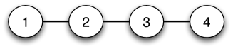
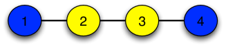
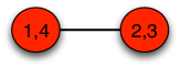
Figure 1: Top panel: the chain topology network of $4$ nodes. Middle panel: poly-synchronous subspace identified by $\mathcal{M}_{2}$. Bottom panel: equivalent network and synchronous subspace identified by $\mathcal{M}_{1}$.

III.2 Generalizations using virtual systems

The results presented in the previous sections link the symmetries of a dynamical system and contraction. Specifically, they show that if a system presents a set of $s>1$ symmetries, then the final behavior is determined by the contraction properties of the vector field.

In this Section, we extend the previous results and show that in order for the solutions of (1) to exhibit a specific symmetry, equivariance and contraction of $f$ are not necessarily needed. Indeed, such a condition can be replaced by a weaker condition: namely, an equivariance condition on the vector field of some auxiliary (or virtual) system, similar in spirit to Theorem 2.

Theorem 9.

Consider the system

$$\dot{y}=v(y,x,t)$$ (7)

where $x(t)$ are the solutions of (1) and $v(x,y,t)$ is some smooth function such that:

$$v(x,x,t)=f(x,t)$$

The following statements hold:

• if $v(y,x,t)$ is $\gamma$-equivariant and contracting towards $\mathcal{M}_{\gamma}$, then any solution of (1) converges towards a $\gamma$-symmetric solution;

• if $v(y,x,t)$ is $h$-equivariant and contracting, then any solution of (1) converges towards a $h$-symmetric solution.

System (7) is termed as virtual system.

Proof.

Indeed, by assumption, all the solutions $y(t)$ of the virtual system globally exponentially converge towards some $h$ ($\gamma$) symmetric solution, say $x(t)$. Now, notice that any solution of (1), say $a(t)$, is a particular solution of (7), since $v(x,x,t)=f(x,t)$. This implies that:

$$\left|a(t)-x(t)\right|\rightarrow 0$$

as $t\rightarrow+\infty$. The result is then proved. ∎

Note that

• Any solution of the virtual system having symmetric initial conditions, i.e. $y(0)=\gamma y(0)$, preserves the symmetry for any $t>0$. In particular, if a solution of the real system has initial conditions verifying the symmetry of the virtual system, i.e. $x_{0}=\gamma x_{0}$, then it preserves this symmetry, i.e. $x(t)=\gamma x(t)$ for any $t\geq 0$. This is a generalization of the basic result presented in Section II.2.

• Theorem 9 can be straightforwardly extended to the case where the virtual system presents a set of $s>1$ spatial symmetries. Analogous results to theorems 6 - 8 can be easily proven.

A discussion on symmetries of virtual systems

Let us briefly discuss some of the main features of our results involving the use of virtual systems.

We showed that a given dynamical system of interest can exhibit some symmetric final behavior even if the corresponding vector field is not equivariant and/or contracting. Indeed, a sufficient condition for a system to exhibit a symmetric final behavior is the symmetry of the vector field of some appropriately constructed virtual system. Of course, an interesting general question is that of identifying a virtual system explaining the final behavior of a real system, an aspect is reminiscent of the process of identifying a Lyapunov function in stability analysis.

The idea of relating behaviors of real systems using a symmetric virtual system, possibly of different dimension, presents analogies with the concept of supersymmetry in particle physics (see e.g. Freund (1988); Ryder (1996) and references therein). The motivation beyond the concept of supersymmetry is that non-symmetric transformations of an object (the real system in our framework) in a finite dimensional space, may be explained by a symmetric transformation of another, possibly higher-dimensional object (the virtual system in our framework).

Finally, we remark here that all the results presented above can be straightforwardly extended to address the problem of designing control strategies guaranteeing convergence of a system of interest onto some desired trajectory. Intuitively, the idea is that the control input has to: i) generate some desired symmetry for the vector field (and hence some desired invariant subspace defining the system’s final behavior); ii) drive all the trajectories towards the invariant subspace imposing contraction.

IV System with inputs

In the above sections, we presented some results that can be used to analyze the final behavior of a system of interest. The main idea beyond such results is the use of contraction to study convergence of trajectories towards some invariant subspace. In turn, such a subspace is defined by some structural property of the vector field, namely a symmetry.

We now generalize this result further, and show that it is possible to determine a direct relation between the trajectories of a system when forced by different classes of inputs. The results presented in this Section are also based on the concept of virtual system. Indeed, while the forced systems of interest considered here are not equivariant and/or contracting, we will show that it is possible to construct a symmetric and contracting virtual system which allows us to relate the final behavior of the two systems.

Consider a system described by:

$$\dot{x}=f(x,u(t),t)$$ (8)

The following result holds:

Theorem 10.

Assume that (8) is contracting with respect to $x$, uniformly in $u(t)$, and that there exist some linear transformations $\gamma_{i}$, $\rho_{i}$, $i\geq 1$, such that: $\gamma_{i}f(x,u(t),t)=f(\gamma_{i}x,\rho_{i}u(t),t)$ Let $x_{i}(t)$ be solutions of (8) when forced by $u(t)=u_{i}(t)$, i.e. $\dot{x}_{i}=f(x_{i},u_{i}(t),t),\quad x_{i}(t=0)=x_{0,i}$. Then, for any $u_{i}(t)$, $u_{j}(t)$ such that $\rho_{i}u_{i}(t)=\rho_{j}u_{j}(t)$

$$\left|\gamma_{i}x_{i}-\gamma_{j}x_{j}\right|\rightarrow 0$$

as $t\rightarrow+\infty$. Moreover, let $x_{i}^{k}$ and $x_{j}^{k}$ the $k$-th component of $x_{i}$ and $x_{j}$ respectively and $\gamma_{i}^{k}$, ($\gamma_{j}^{k}$) be the $k$-th component of $\gamma_{i}$ ($\gamma_{j}$). If $\gamma_{i}^{k}x_{0,i}^{k}=\gamma_{j}^{k}x_{0,j}^{k}$. then $\gamma_{i}^{k}x_{i}^{k}(t)=\gamma_{j}^{k}x_{j}^{k}(t)$, for any $t\geq 0$.

The second statement of the above Theorem implies that if the system when forced by two different inputs starts with certain symmetries, then the symmetries are preserved.

Proof.

Indeed, let $u_{v}=\rho_{i}u_{i}=\rho_{j}u_{j}$ and consider the following virtual system:

$$\dot{y}=f(y,u_{v},t)$$ (9)

Notice that, for any $i$, $j$, $\gamma_{i}x_{i}$ and $\gamma_{j}x_{j}$ are particular solutions of such a system. Indeed:

$$\begin{array}[]{*{20}l}\gamma_{i}\dot{x}_{i}=\gamma_{i}f(x_{i},u_{i},t)=f(\gamma_{i}x_{i},\rho_{i}u_{i},t)=f(\gamma_{i}x_{i},u_{v},t)\\ \gamma_{j}\dot{x}_{j}=\gamma_{j}f(x_{j},u_{j},t)=f(\gamma_{j}x_{j},\rho_{j}u_{j},t)=f(\gamma_{j}x_{j},u_{v},t)\\ \end{array}$$

Now, since $f(x,u_{v},t)$ is contracting by hypotheses, we have, for any $i$, $j$, there exists some $C$ such that:

$$\left|\gamma_{i}x_{i}-\gamma_{j}x_{j}\right|\leq C\left|\gamma_{i}x_{0,i}-\gamma_{j}x_{0,j}\right|e^{-\lambda t},\quad\lambda>0$$

This proves the first part of the result. To conclude the proof it suffices to notice that exponential convergence of $\left|\gamma_{i}x_{i}-\gamma_{j}x_{j}\right|$ to $0$ implies that all of its components exponentially converge to $0$. In particular, this implies that there exists some $C_{k}$, $\lambda_{k}$ such that:

$$\left|\gamma_{i}^{k}x_{i}^{k}-\gamma_{j}^{k}x_{j}^{k}\right|\leq C_{k}\left|\gamma_{i}^{k}x_{0,i}^{k}-\gamma_{j}^{k}x_{0,j}^{k}\right|e^{-\lambda t_{k}},\quad\lambda_{k}>0$$

Since $\left|\gamma_{i}^{k}x_{0,i}^{k}-\gamma_{j}^{k}x_{0,j}^{k}\right|=0$ by hypotheses, we have that $\left|\gamma_{i}^{k}x_{i}^{k}(t)-\gamma_{j}^{k}x_{j}^{k}(t)\right|$, $\forall t\geq 0$ ∎

Theorem 10 can be extended by replacing the linear operators $\gamma_{i}$, $\rho_{i}$ by more general nonlinear transformations acting on the system

$$\dot{x}=f(x,u(x,t),t)$$ (10)

The transformations considered are smooth nonlinear functions of the state and of time, $\gamma=\gamma(x,t)$, $\rho=\rho(u(x,t),x,t)$ Following the same arguments as in Theorem 10, it is then straightforward to show,

Theorem 11.

Assume that (10) is contracting uniformly in $u(x,t)$ and that there exist some $\gamma_{i}(x,t)$, $\rho_{i}(u(x,t),x,t)$, $i\geq 1$, such that:

$$\frac{\partial\gamma_{i}}{\partial x}f(x,u(x,t),t)=f(\gamma_{i}(x),\rho_{i}(u(x,t),x,t),t)$$

Let $x_{i}(t)$ be solutions of (10) when forced by $u(t)=u_{i}(x_{i},t)$, i.e. $\dot{x}_{i}=f(x_{i},u_{i}(x_{i},t),t)$, $x_{i}(t=0)=x_{0,i}$ Then, for any $u_{i}(x_{i},t)$, $u_{j}(x_{j},t)$ such that $\rho_{i}(u(x_{i},t),x_{i},t)=\rho_{j}(u_{j}(x_{j},t),x_{j},t)$

$$\left|\gamma_{i}(x_{i})-\gamma_{j}(x_{j})\right|\rightarrow 0$$

as $t\rightarrow+\infty$. Moreover, let $x_{i}^{k}$ and $x_{j}^{k}$ the $k$-th component of $x_{i}$ and $x_{j}$ respectively and $\gamma_{i}^{k}$, ($\gamma_{j}^{k}$) be the $k$-th component of $\gamma_{i}$ ($\gamma_{j}$). If

$$\gamma_{i}^{k}\left(x_{0,i}^{k}\right)=\gamma_{j}^{k}\left(x_{0,j}^{k}\right)$$

then $\gamma_{i}^{k}\left(x_{i}(t)^{k}\right)=\gamma_{j}^{k}\left(x_{j}(t)^{k}\right)$, for any $t\geq 0$.

Proof.

The proof follows exactly the same steps as those used to prove Theorem 10, with $u_{v}$ in virtual system (9) now being chosen as $u_{v}=\rho_{i}(u(x_{i},t),x_{i},t)=\rho_{j}(u_{j}(x_{j},t),x_{j},t)$. ∎

We close this Section by pointing out some features of the above two theorems.

• the proofs of both Theorem 10 and Theorem 11 are based on the proof of contraction of some appropriately constructed virtual system of the form (9). We now show that, if some hypotheses are made on $\gamma_{i}$’s, then the contraction condition can be weakened. Specifically, assume that all the intersection of the subspaces defined by $\gamma_{i}$, $\mathcal{M}_{i}$, is nonempty. Then, it is straightforward to check that $\left|\gamma_{i}x_{i}-\gamma_{j}x_{j}\right|\rightarrow 0$ if: (i) $f$ is contracting towards each $\mathcal{M}_{i}$, or (ii) contracting towards $\mathcal{M}_{\cap}$. Notice that, since our results make use of symmetries of virtual systems, they extend those in Gerard and Slotine ;

• Analogously, Theorem 10 and Theorem 11 can also be extended to study the case where the input $u_{i}$ selects one specific symmetry $\gamma_{i}$. Indeed, let $u_{v}=\rho_{i}u_{i}$. In this case, it can be shown that symmetry $\gamma_{i}$ is shown by the solutions of (8) if $f(x,u_{v},t)$ is contracting towards $\mathcal{M}_{i}$.

• A particularly interesting case for Theorem 10 is when some of the components of $x_{0,i}$ and $x_{0,j}$ are the same and the actions $\gamma_{i}$ and $\gamma_{j}$ leave such components unchanged. That is, in view of the notations above $\gamma_{i}^{k}=id=\gamma_{j}^{k}$ and $x_{0,i}^{k}=x_{0,j}^{k}$. Indeed, in this case Theorem 10 implies that $x_{i}^{k}(t)=x_{j}^{k}(t),$ $\forall t\geq 0$ That is, the $k$-th components of the trajectories of (8) have identical temporal evolutions even if forced by different inputs. A similar result holds for Theorem 11 .This consequence of the above two results is used in Section V.

V An example: invariance under input scaling

In a series of recent papers, input-output properties of some cellular signaling biochemical systems have been analyzed Goentoro et al. (2009); Shoval et al. (2010); Goentoro and Kirschner (2009); Cohen-Saidon et al. (2009). Such studies point out that many sensory systems show the property of having their output invariant under input scaling, which can be formally defined as follows:

Definition 4.

Let $x_{i}(t)$, $x_{j}(t)$ be solutions of (8) with initial conditions $x_{0}=x_{i}(0)=x_{j}(0)$, when $u(t)=\chi_{i}(t)$ and $u(t)=\chi_{j}(t)$, respectively. System (8) is invariant under input scaling if $x_{i}(t)=x_{j}(t)$ for any $\chi_{i}(t)$, $\chi_{j}(t)$ such that $\chi_{j}(t)=F(t)\chi_{i}(t)$, with $F(t)>0$.

Invariance under input scaling with constant $F(t)=F$ has been recently studied in transcription networks by Alon and his co-authors Goentoro et al. (2009); Cohen-Saidon et al. (2009); Shoval et al. (2010). In such papers, the authors focus on the study of transcriptional networks subject to step-inputs. In this case, the invariance under input scaling is called fold-change detection behavior (FCD), as the output of the system depends only on fold changes in input and not on its absolute level. For example, if the input to the system is a step function from $1$ to $2$, then its output is the same as if the step was increased from $2$ to $4$.

This section uses this paper’s results to analyze the associated mathematical models, arising from protein signal-transduction systems and bacterial chemotaxis, and in particular it revisits the recent work Shoval et al. (2010) from this point of view. It also shows how these results could, for instance, suggest a mechanism for stable quorum sensing in bacterial chemotaxis, thus combining symmetries in cell interactions (quorum sensing) with invariance to input scaling (fold change detection).

V.1 Gene regulation

This first example considers a pattern (network motif) arising in gene regulation networks, the Type $1$ Incoherent Feed-Forward Loop (I1-FFL) Eichenberger et al. (2004), Milo et al. (2002). The I1-FFL is one of the most common network motifs in gene regulation networks (see also Section VII). As shown in Figure 2, it consists of an activator, $X$, which controls a target gene, $Z$, and activate a repressor of the same gene, $Y$ (which can be thought of as the output of the system). It has been recently shown that such a network motif can generate a temporal pulse of $Z$ response, accelerate the response time of $Z$ and act as a band-pass amplitude filter, see e.g. Mangan et al. (2006), Kim et al. (2008).

In Goentoro et al. (2009) it has also been shown by using a dimensionless analysis that for a certain range of biochemical parameters, the I1-FFL can exhibit invariance under step-input scaling (i.e. FCD).

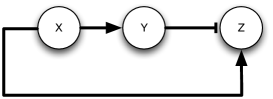
Figure 2: A schematic representation of the I1-FFL

V.1.1 A basic model

In Goentoro et al. (2009), it was shown that a minimal circuit which achieves FCD is the I1-FFL, with the activator in linear regime and the repressor saturating the promoter of the target gene, $Z$. The model in Goentoro et al. (2009) is of the form

$$\begin{array}[]{*{20}l}\dot{Y}=-\alpha_{1}Y+\chi(t)\\ \dot{Z}=\beta_{2}\frac{\chi(t)}{Y}-\alpha_{2}Z\end{array}$$ (11)

where $\alpha_{1}$, $\alpha_{2}$, $\beta_{2}$ are biochemical (positive) parameters and $\chi(t)$ is the input to the system (which can be approximated by the concentration of $X$). It was also shown that the dimensionless model

$$\begin{array}[]{*{20}c}\frac{dy}{d\tau}=F-y\\ r\frac{dz}{d\tau}=\frac{F}{y}-z\end{array}$$

with:

$$\begin{array}[]{*{20}l}y=\frac{Y\alpha_{1}}{\beta_{1}\chi_{\min}}&Z=\frac{Z}{\beta_{2}\alpha_{1}/\beta_{1}\alpha_{2}}\\ F=\frac{\chi(t)}{\chi_{\min}}&\tau=\alpha_{1}t\end{array}$$

exhibits invariance under input scaling. Later we will also consider more detailed mathematical models that in Goentoro et al. (2009) have been analyzed numerically. In Section VII, we will also analyze other important network motifs under a slightly different viewpoint, i.e. by considering each of the species composing the motif as nodes of an interconnected systems.

In this Section, we show invariance under input scaling for system (11) for any input, $\chi_{i}(t)$, $\chi_{j}(t)$, such that $\frac{\chi_{i}(t)}{\chi_{\min,i}}=\frac{\chi_{j}(t)}{\chi_{\min,j}}=F(t)$ In the above expressions $\chi_{\min,i}$ and $\chi_{\min,j}$ denote the basal level of the inputs $\chi_{i}(t)$ and $\chi_{j}(t)$ respectively. Such levels are assumed to be nonzero. Notice that the above class of inputs is wider that the one used in Definition 4.

Theorem 10 is now used to prove invariance under input scaling for (11). That is, we show that invariance under input scaling is a consequence of the existence of a symmetric and contracting virtual system in the spirit of Theorem 10.

In what follows, we will denote with $x_{i}=(Y_{i},Z_{i})^{T}$ and $x_{j}=(Y_{j},Z_{j})^{T}$ the solutions of (11), when $\chi(t)=\chi_{i}(t)$ and $\chi(t)=\chi_{j}(t)$, respectively. We assume that $Z_{i}(0)=Z_{j}(0)$. In terms of the notation introduced in Theorem 10, we have $u(t)=\chi(t)$ and:

$$f(x,u(t))=\left(\begin{array}[]{*{20}c}-\alpha_{1}Y+\chi(t)\\ \beta_{2}\frac{\chi(t)}{Y}-\alpha_{2}Z\\ \end{array}\right)$$

Now, define the following actions:

$$\begin{array}[]{*{20}c}\gamma_{i}=\left(\begin{array}[]{*{20}c}Y\\ Z\\ \end{array}\right)\rightarrow\left(\begin{array}[]{*{20}c}\frac{Y}{\chi_{\min,i}}\\ Z\\ \end{array}\right),&\rho_{i}:\chi(t)\rightarrow\frac{\chi(t)}{\chi_{\min,i}}=F(t)\end{array}$$ (12)

It is straightforward to check that:

• $f(x,u(t))$ is contracting uniformly in $u(t)$;

• $\gamma_{i}f(x_{i},\chi_{i}(t))=f(\gamma_{i}x_{i},\rho_{i}\chi_{i}(t))$

Now, Theorem 10 implies that for any input $\chi_{i}(t)$, $\chi_{j}(t)$ such that $\rho_{i}\chi_{i}(t)=\rho_{j}\chi_{j}(t)$, $\gamma_{i}x_{i}$ and $\gamma_{j}x_{j}$ globally exponentially converge towards each other. That is:

$$\left|\gamma_{i}x_{i}-\gamma_{j}x_{j}\right|=\left|\left(\begin{array}[]{*{20}c}\frac{Y_{i}}{\chi_{\min,i}}-\frac{Y_{j}}{\chi_{\min,j}}\\ Z_{i}-Z_{j}\end{array}\right)\right|\rightarrow 0$$ (13)

for any $\chi_{i}$, $\chi_{j}$ such that:

$$\frac{\chi_{i}(t)}{\chi_{\min,i}}=\frac{\chi_{j}(t)}{\chi_{\min,j}}=F(t)$$ (14)

Now, (13) implies that $\left|Z_{i}-Z_{j}\right|\rightarrow 0$ exponentially. Since the initial conditions of $Z_{i}$ and $Z_{j}$ are the same we have that $Z_{i}(t)=Z_{j}(t)$ for any $t\geq 0$. That is, the system exhibits invariance under input scaling.

V.2 A model from chemotaxis

In bacterial chemotaxis, bacteria walk through a chemo-attractant field, say $u(t,r)$ (r denotes two dimensional space vector). Along their walk, bacteria sense the concentration of $u$ at their position and compute the tumbling rate (rate of changes of the direction) so as to move towards the direction where the gradient increases, see e.g. Celani and Vergassola (2010). Typically, the input field is provided by means of a source of attractant which diffuses in the medium with bacteria accumulating in the neighborhood of the source. In this case, the information on the position of the source is encoded only in the shape of the field and not in its strength. Therefore, it is reasonable for bacteria to evolve a search pattern which is dependent only on the shape of the field and not on its strength, i.e., a search pattern which is invariant under input scaling Shoval et al. (2010). Specifically, consider the following model Shoval et al. (2010) adapted from the chemotaxis model of Tu et al. (2008):

$$\begin{array}[]{*{20}l}\ \dot{x}=xf(y)\\ \epsilon\dot{y}=\phi\left(\frac{u}{x}\right)-y\\ \end{array}$$ (15)

where $u>0$ is an increasing step-input to the system, representing the ligand concentration, and $y>0$, the output of the system, represents the average kinase activity. The quantity $x>0$ is an internal variable. We assume the function $\phi$ to be: i) a decreasing function in $x$ with bounded partial derivative $\partial\phi/\partial x$; ii) an increasing function of $u/x$, with derivative $\phi^{\prime}=\partial\phi/\partial(u/x)\leq b$, $b>0$. Note that the above model becomes the one used in Shoval et al. (2010), when $\phi(u/x)=u/x$. Such a model is obtained assuming $x$ is sufficiently large, with the term $u/x$ actually a simplification of a term of the form $u/(x+\eta)$, with $0<\eta\ll x$. The positive constant $\epsilon$ is typically small, so as to represent a separation of time-scales.

Assume as in Tu et al. (2008) that $f(1)=0$ and that $f(y)$ is strictly increasing with $y$. Obviously, (15) verifies the symmetry conditions of Theorem 10 with:

$$\begin{array}[]{*{20}c}\gamma_{i}:(x_{i},y_{i})\rightarrow\left(\frac{x_{i}}{\bar{u}_{i}},y_{i}\right)&\ \ \ \ \ \rho_{i}:u_{i}\rightarrow\frac{u_{i}}{\bar{u}_{i}}\end{array}$$ (16)

where $\bar{u}_{i}$ denotes the initial (lower) value, at time $t=0$, of the step function. As in the previous Section we assume that $y_{i}(0)=y_{j}(0)$. Now, by means of Theorem 10, we can conclude that, if the system is contracting, $y_{i}(t)=y_{j}(t)$, $\forall t\geq 0$, for any input such that $\frac{u_{i}}{\bar{u}_{i}}=\frac{u_{j}}{\bar{u}_{j}}=F$.

Let us derive a condition for (15) to be contracting, which will give conditions on the dynamics and inputs of (15) ensuring invariance under input scaling. Model (15) can be recast as

$$\ddot{y}+\frac{1}{\epsilon}\dot{y}-\frac{1}{\epsilon}\frac{\partial\phi}{\partial x}xf(y)=0$$ (17)

As in Tu et al. (2008); Shoval et al. (2010), choose $f(y)=y-1$ for simplicity, so that (17) becomes

$$\ddot{y}+\frac{1}{\epsilon}\dot{y}-\frac{1}{\epsilon}\frac{\partial\phi}{\partial x}x(y-1)=0$$ (18)

The above dynamics is similar to a mechanical mass-spring-damper system with a time-varying spring, $\ddot{r}+2\eta\omega\dot{r}+\omega^{2}r=0$ with $2\eta\omega=\frac{1}{\epsilon}$ and $\omega^{2}=-\frac{1}{\epsilon}\frac{\partial\phi}{\partial x}x$. Now, as shown in Lohmiller and Slotine such a dynamics is contracting if $\eta>\frac{1}{\sqrt{2}}$. Thus, it immediately follows that (18) is contracting if:

$$\frac{\partial\phi}{\partial x}x>-\frac{1}{2\epsilon}$$ (19)

Hence, contraction is attained if $\phi^{\prime}\left(-\frac{u}{x^{2}}\right)x>-\frac{1}{2\epsilon}$ That is, a sufficient condition for (18) to be contracting is

$$x>2\epsilon ub$$ (20)

Notice that, in the case where $\phi\left(u/x\right)=u/x$, (20) simply becomes:

$$x>2\epsilon u$$ (21)

The above inequality implies that, in this case, the system is contracting (and hence exhibits invariance under input scaling) if the level of $x$ is sufficiently high (which is true by hypotheses) and its dynamics is sufficiently slow ($\epsilon$ small) with respect to the dynamics of $y$. Also, given $\varepsilon<\frac{1}{2}$ and a constant $u$, if contraction condition (21) is verified at $t=0$ with initial conditions embedded in a ball contained in the contraction region (21), it remains verified for any $t\geq 0$.

Finally, note that the results of this section, and indeed of the original Goentoro et al. (2009); Shoval et al. (2010), are closely related to the idea, first introduced in Pham and Slotine (2007) and further studied in Gerard and Slotine , of detecting a symmetry (here, in the environment) by using a dynamic system having the same symmetry.

VI Analysis and control of interconnected systems

The results presented in the previous Section indicate that there exists a direct link between symmetries of a (virtual) vector field and of its solutions, if the system is contracting (or it is made contracting by some control input).

The aim of this Section is that of using the above results to analyze and control the (poly-) synchronous behavior of $N>1$ (possibly heterogeneous) interconnected systems (also termed as networks in what follows). Such a behavior has been recently reported in ecological systems, networks characterized by strong community structure and in bipartite networks consisting of two groups (see e.g. Montbrió et al. (2004); Oh et al. (2005); Sorrentino and Ott (2007)). For interconnected systems, symmetries are essentially defined by the nodes’ dynamics, the topology of the network and by the particular choice of the coupling functions.

As a first step we will introduce the notion of interconnected system that will be used in the following, see also Golubitsky and Stewart (2006).

VI.1 Definitions

In our framework the phase space of the $i$-th node (or cell, or neuron) is denoted with $P_{i}$, while its state at time $t$ is denoted with $x_{i}(t)$. Notice that $P_{i}$ could in general be a manifold. Each node has an intrinsic dynamics, which is affected by the state of some other nodes (i.e. the neighbors of $i$) by means of some coupling function. Those interactions will be represented by means of directed graphs. In such a graph the nodes having the same internal dynamics will be represented with the same symbol. Analogously, heterogeneous coupling functions can be taken into account: identical functions will be denoted by the same symbol.

This is formalized with the following:

Definition 5.

An interconnected system consists of: (i) a set of nodes $\mathcal{N}=\left\{1,\ldots,N\right\}$; (ii) an equivalence relation, $\sim_{\mathcal{N}}$ on $\mathcal{N}$; (iii) a finite set, $\mathcal{E}$, of edges (arrows); (iv) an equivalence relation, $\sim_{\mathcal{E}}$ on $\mathcal{E}$; (v) the maps $\mathcal{H}:\mathcal{E}\rightarrow\mathcal{N}$ and $\mathcal{T}:\mathcal{E}\rightarrow\mathcal{N}$ such that: for $e\in\mathcal{E}$, we have $\mathcal{H}(e)$ is the head of the arrow and $\mathcal{T}(e)$ the tail of the arrow; (vi) equivalent arrows have equivalent tails and heads. That is, if $e_{1},e_{2}\in\mathcal{E}$ and $e_{1}\sim_{\mathcal{E}}e_{2}$, then $\mathcal{H}(e_{1})\sim_{\mathcal{N}}\mathcal{H}(e_{2})$ and $\mathcal{T}(e_{1})\sim_{\mathcal{N}}\mathcal{T}(e_{2})$.

We say that an edge $e\in\mathcal{E}$ is an input edge to a node, say $i$, if $\mathcal{H}\left(e\right)=i$. The set of input edges to node $i$ is termed as input set and denoted by $\mathcal{I}\left(i\right)$. We also say that two nodes, say $c$ and $d$, are input-equivalent if there exists an arrow type preserving bijection, $\beta:\mathcal{I}(c)\rightarrow\mathcal{I}(d)$.

Finally, our set-up is completed by defining the dynamics of an interconnected system as follows:

Definition 6.

The dynamical system

$$\dot{X}=F(X,t)$$ (22)

defines an interconnected system if its phase space is defined as $P=P_{1}\times\ldots P_{N}\times{\mathbb{R}}^{+}$ where $P_{i}$ denotes the phase space of the $i$-th network node. Furthermore, let $\pi_{i}:P\rightarrow P_{i}$ be projections of (22), then it must hold that $\pi_{i}(X(t))=x_{i}(t)$.

VI.2 Analysis and control

Let: $P_{1}\subseteq{\mathbb{R}}^{n_{1}}$, $P_{2}\subseteq{\mathbb{R}}^{n_{2}}$, $\ldots$, $P_{N}\subseteq{\mathbb{R}}^{n_{N}}$ be convex subsets, $P=P_{1}\times\ldots\times P_{N}$, $X=[x_{1}^{T},\ldots,x_{N}^{T}]^{T}$, $x_{i}\in P_{i}$, $\phi_{i}:P\times{\mathbb{R}}^{+}\rightarrow P_{i}$ be smooth functions. In what follows, we consider systems of the form:

$$\dot{x}_{i}=\phi_{i}(X,t)=f_{i}(x_{i},t)+\tilde{h}_{i}(X,t)$$ (23)

with $i=1,\ldots,N$. Notice that (23) represents an interconnected system (Definition 6). Specifically, in (23) the function $f_{i}:P_{i}\times{\mathbb{R}}^{+}\rightarrow P_{i}$ is the intrinsic dynamics of the $i$-th node, while the function $\tilde{h}_{i}:P\times{\mathbb{R}}^{+}\rightarrow P_{i}$ describes the interaction of the $i$-th node with the other nodes composing the interconnected system.

Notice that the above formalization allows us to consider within a unique framework directed and undirected networks, self loops and multiple interactions. We will also consider networks with (smoothly) changing topology.

The main idea of this Section for the study of the collective poly-synchronous behavior emerging in network (23) can be stated as follows: (i) study symmetries of (23) to determine the possible patterns of synchrony; (ii) determine among the possible patterns, the one exhibited by (23) using contraction properties.

Consider a partition of the $N$ nodes of a network into $k$ groups, $\mathcal{G}_{1},\ldots,\mathcal{G}_{k}$, characterized by the same intrinsic dynamics. We define the following invariant subspaces associated to each group of nodes:

$$\mathcal{M}_{p,s}=\left\{x_{i}=x_{j},\quad\forall i,j\in\mathcal{G}_{s}\right\},\quad s=1,\ldots,k$$

Notice that all the nodes of the $i$-th group are synchronous if and only if network dynamics evolve onto the associated subspace $\mathcal{M}_{p,i}$. The poly-synchronous subspace, say $\mathcal{M}_{p}$, is then defined as the intersection of all $\mathcal{M}_{p,s}$, i.e. $\mathcal{M}_{p}=\cap_{s}\mathcal{M}_{p,s}$, or equivalently

$$\mathcal{M}_{p}=\left\{x_{i}=x_{j},\forall i,j\in\mathcal{G}_{m},1\leq m\leq k\right\}$$

We a say that a pattern of synchrony is possible for the network of interest if its corresponding poly-synchronous subspace is flow invariant. In this view, a useful result is the following:

Theorem 12.

The set $\mathcal{M}_{p}$ is invariant for network (22) if the nodes belonging to group $\mathcal{G}_{p}$: i) have the same uncoupled dynamics; ii) are input-equivalent.

The proof of the above result can be found in e.g. Golubitsky and Stewart (2003, 2006). In terms of network synchronization, intuitively such a result implies that a specific pattern of synchrony is possible if the aspiring synchronous nodes have synchronous input sets.

The following result is a straightforward consequence of the results of the previous Section on spatial symmetries.

Corollary 1.

Assume that for network (23) the sets $\mathcal{M}_{p,s}$ exist. Then, the synchrony pattern exhibited by the network is given by: (i) $\mathcal{M}_{p}$, if the network is contracting, or contracting towards each $\mathcal{M}_{p,s}$; (ii) $\mathcal{M}_{p,s}$, if the network is contracting towards $\mathcal{M}_{p,s}$.

One of the applications where the above results can be used is that of designing networks performing specific tasks. For example, in Pham and Slotine (2007) it was shown that a network with a specific symmetry can be used to detect symmetries of e.g. images. Our results can be used to extend this framework. Indeed, each network node (23) may be used to process some exogenous input, $U(t)=[u_{1},\ldots,u_{N}]$, i.e.

$$\dot{x}_{i}=\phi_{i}(X,t)=f_{i}(x_{i},t)+\tilde{h}_{i}(X,t)+u_{i}(t)$$

Now, while $u_{i}$ denotes the information that has to be processed by node $i$, the couplings $\tilde{h}_{i}$ may be seen as an input (typically, sparse) acting on the couplings between nodes, so as to activate a desired, arbitrary, symmetry. The output of the network is then some desired synchronous pattern which arises from the intersection of the symmetries activated by $\bar{U}(t)$ and those activated by $\tilde{U}(X)$. Figure 3 schematically illustrates this principle.

Figure 3: A schematic representation of a network used to process information. In our framework, the network is subject to two kinds of inputs: $\bar{U}(t)$ and $\tilde{U}(X)$. In particular, $\bar{U}(t)$ can be seen as the information processed by the network: such input can activate some intrinsic symmetries of the network. On the other hand, $\tilde{U}(X)$ is a typically sparse input that acts on the coupling functions so as to force the activation of some desired symmetry of the interconnected system.

For instance, assume that the system consists of a large number of synchronized oscillators. Then we know Wang and Slotine (2005) that with an adequate choice of coupling gains:

• adding a single inhibitory connection between any two nodes will make the entire system contracting and therefore will stop the oscillations.

• adding a ”leader” oscillator (i.e., an oscillator with only feed-foward connections to the rest of the network, its neighbors for instance) will make the entire system get in phase with the leader.

Thus very sparse feedback inputs can completely change the symmetries of the system, and therefore its symmetry detection specifications.

Chain topologies: revised

Consider, again, the network topology in Figure 1. Recall that in Section III.1.1 we proved network synchronization in two subsequent steps. Specifically, we first proved that all network trajectories are globally exponentially convergent towards the poly-synchronous subspace where $x_{1}=x_{4}$, $x_{2}=x_{3}$. We then showed that network dynamics reduced on such a subspace were globally exponentially convergent towards the synchronous subspace.

The subspaces $\mathcal{M}_{2}$ and $\mathcal{M}_{1}$ towards which convergence was proved were, in turn, determined by equivariance of network dynamics with respect to some permutation action. Notice that this equivariance property is a direct consequence of the fact that node $1$ of the network is input-equivalent to node $4$ and node $2$ is input-equivalent to node $3$. Moreover, the equivalent nodes of the $2$-nodes reduced network are also input-equivalent.

VII Applications

VII.1 Synchrony patterns for distributed computing

We now turn our attention to the problem of imposing some poly-synchronous behavior for a network of interest. Specifically, we will impose different patterns of synchrony for a network composed of Hopfield models. The motivation that we have in mind here is that of multi-purpose networks, i.e. networks that can be reused to perform different tasks. For example, this may be the case of sensor networks (Martinelli (2008), Yarvis et al. (2005)) where each poly-synchronous steady steady is associated to a specific set of inputs. A further notable example is the brain, where different poly-synchronous behaviors are believed to play a key role in e.g. learning processes (see e.g. Izhikevich (2006)).

We consider here a network of Hopfield models Hopfield (1982), Oshima and Odagaki (2007):

$$\dot{x}_{i}=-x_{i}+\sum_{j\in N_{i}}a_{ij}(t)h_{ij}(x_{i},x_{j},t)+u_{i}$$ (24)

where $a_{ij}(t)$ is the $i$-th element of the time-varying interconnection matrix $A(t)$, $h_{ij}$ represents the interconnection function from node $j$ to node $i$ and $u_{i}$ in an exogenous input to the $i$-th node.

We start with the network in Figure 4. Nodes denoted by the same shape are forced by the same exogenous input. Specifically: (i) $u_{i}(t)=1+\sin(0.7t)$ for the circle nodes; (ii) $u_{i}(t)=5+3\sin(0.5t)$ for the square nodes; (iii) $u_{i}(t)=0$ for node $13$.

Analogously, identical arrows denote identical coupling functions:

• the coupling between circle nodes is diffusive, bidirectional and linear: $h_{ij}(x_{i},x_{j},t)=a_{ij}(t)(x_{j}-x_{i})$

• the coupling between square nodes is diffusive, unidirectional and linear;

• the coupling between circle and square nodes is diffusive, bidirectional and nonlinear: $h_{ij}(x_{i},x_{j},t)=a_{ij}(t)\left(\arctan(x_{j})-\arctan(x_{j})\right)$

• the square nodes affect the dynamics of node $13$ unidirectionally. Specifically, the dynamics of $x_{13}$ is given by:

  $$\dot{x}_{13}=-x_{13}+(1-b(t))\sum_{j=9}^{12}\frac{x_{j}}{1+x_{j}}+b(t)\sum_{j=9}^{12}\frac{1}{1+x_{j}}$$ (25)

  where $b(t)$ is a parameter that is smoothly increased between $0$ and $1$. Notice that $b(t)$ can be used to switch between two different coupling functions.

We remark here that the input to node $13$ is a well known coupling mechanism in the literature on neural networks, and is termed as excitatory-only coupling, see e.g. Rubin (2006).

It is straightforward to check that network dynamics are contracting (using e.g. the matrix measure induced by the $1$-norm).

Figure 4: Network of Hopfield models used in Section VII.1 (top panel). The input-equivalent nodes are pointed out in the bottom panel.

In Figure 4 (right panel) the input-equivalent nodes are pointed out by means of colors: the associated linear poly-synchronous subspace is

$$\begin{array}[]{*{20}l}\mathcal{M}_{1}=\left\{x_{i}=x_{j},i,j=1,\ldots,8\right\}\bigcap\\ \bigcap\left\{x_{i}=x_{j},i,j=9,\ldots,12\right\}\end{array}$$

Furthermore, it is easy to check that $\mathcal{M}_{1}$ is flow invariant. Now, since network dynamics are contracting, all of its trajectories converge towards a unique solution embedded into $\mathcal{M}_{1}$. That is, at steady state all the nodes having the same color in Figure 4 are synchronized. Figure 5 (left panel) clearly confirms the theoretical analysis, showing the presence of the three synchronized clusters, when $b(t)=0$.

The same synchronized behavior is kept even when $b(t)$ smoothly varies from $0$ to $1$. Indeed, network dynamics is still contracting and the input-equivalence propertydefining $\mathcal{M}_{1}$ is preserved. In Figure 5 (right panel) the behavior of the network is shown when at $t=50$, $b(t)$ is set to $1$.

Notice that the variation of $b(t)$ from $0$ to $1$ causes an inhibitory effect of the level of $x_{13}$. This is due to the fact that, when $b(t)=0$, $x_{13}$ is forced by the sum of increasing sigmoidal functions. Vice-versa, when $b(t)=1$, $x_{13}$ is forced by the sum decreasing sigmoidal functions.

Now, assume that we need to create a new synchronized cluster consisting of e.g. nodes $2$, $4$, $6$, $8$. A way to achieve this task is that of modifying the input-equivalence property defining $\mathcal{M}_{1}$ and to impose a new input-equivalence defining the subspace

$$\begin{array}[]{*{20}l}\mathcal{M}_{2}=\left\{x_{i}=x_{j},i,j=1,3,5,7\right\}\bigcap\\ \bigcap\left\{x_{i}=x_{j},i,j=2,4,6,8,\right\}\bigcap\\ \bigcap\left\{x_{i}=x_{j},i,j=9,\ldots,12\right\}\end{array}$$

In turn, this can be done by smoothly varying the topology of the network, e.g. by diffusively coupling node $13$ to the nodes $2$, $4$, $6$, $8$. The coupling function used to this aim, which preserves the contracting property, is:

$$h_{i}(x_{i},x_{j})=h(x_{j})-h(x_{i}),\ \ \ h(x)=\frac{1-e^{-x}}{1+e^{-x}}$$

In Figure 6 (left panel) the new topology is shown, together with the class of input-equivalence. The same Figure (right panel) shows the behavior of the network, pointing out that a new cluster of synchronized nodes arises.

\psfrag{x}[c]{{Time}}\psfrag{y}[c]{{$x_{i}$}}\includegraphics[width=170.71652pt]{simulation_hopfield_0_50}

\psfrag{x}[c]{{Time}}\psfrag{y}[c]{{$x_{i}$}}\psfrag{x}[c]{{Time}}\psfrag{y}[c]{{$x_{i}$}}\includegraphics[width=170.71652pt]{simulation_hopfield_50_90}

Figure 5: Network of Hopfield models (24) when (top panel) $b(t)$ in (25) is equal to $0$. Notice the presence of three synchronized groups of nodes, corresponding the three classes of input-equivalent nodes pointed out in Figure 4. The same synchronized groups are present when $b(t)$ in is switched to $0$ (bottom panel). Notice that, in this case, the change of the coupling modifies the temporal behavior of node $13$.

\psfrag{x}[c]{{Time}}\psfrag{y}[c]{{$x_{i}$}}\includegraphics[width=170.71652pt]{simulation_hopfield_90_150}

Figure 6: Network of Hopfield models used in Section VII.1. Top panel: two new links are activated by node $13$, creating a new class of input-equivalent nodes (in yellow). Bottom panel: temporal evolution of network nodes’ dynamics. Notice the presence of a new group of synchronized nodes, corresponding to the new input-equivalence class.

VII.2 Chemotaxis with quorum

In the above examples, we assumed that each node of the network communicates directly with its neighbors. This assumption on the communication mode is often made in the literature on synchronization, see e.g. Newman (2003); Boccaletti et al. (2006); Danino et al. (2010) and references therein. In many natural systems, however, network nodes do not communicate directly, but rather by means of the environment. This mechanism, known as quorum sensing Miller and Bassler (2001); Nardelli et al. (2008); Russo and Slotine (2010) is believed to play a key role in bacterial infection, as well as e.g. in bioluminescence and biofilm formation Anetzberger et al. (2009); Nadell et al. (2008). Although to our knowledge this has not yet been studied experimentally, plausibly quorum sensing may also play a role in bacterial chemotaxis. Indeed, such a mechanism would enhance robustness of the chemotactic response Tabareau et al. (2010), with respect both to noise (including Brownian noise) and to the large variations in gene expressions between individual cells Tyagu (2010).

From a network dynamics viewpoint, a detailed model of such a mechanism would need to keep track of the temporal evolution of the environmental (shared) quantity, resulting in an additional set of ordinary differential equations Katriel (2008); Russo and Slotine (2010):

$$\begin{array}[]{*{20}l}\dot{x}_{i}=f\left(x_{i},z\right)&i=1,\ldots,N\\ \dot{z}=g\left(z,\Psi\left(X\right),t\right)\end{array}$$ (26)

In the above equation, $N$ is the number of nodes sharing the same environment (medium). The set of state variables of the nodes is $x_{i}$, $X=\left[x_{1}^{T},\ldots,x_{N}^{T}\right]^{T}$, while the set of the state variables of the common medium dynamics is $z$. Notice that the medium dynamics and the medium dynamics can be of different dimensions (e.g. $x_{i}\in{\mathbb{R}}^{n}$, $z\in{\mathbb{R}}^{d}$).The dynamics of the nodes affect the dynamics of the common medium by means of some coupling (or input) function, $\Psi:{\mathbb{R}}^{Nn}\rightarrow{\mathbb{R}}^{d}$. We assume that $\partial f/\partial z$ is bounded (that is, all of its elements are bounded).

In Russo and Slotine (2010) it is shown that synchronization of (26) is attained if the reduced order virtual system

$$\begin{array}[]{*{20}l}\dot{y}=f\left(y,y_{z}\right)\\ \end{array}$$ (27)

is contracting. Notice that the choice of such a reduced order virtual system is made possible by the fact that network equations (26) are symmetric with respect to any permutation of nodes state variables, $x_{i}$.

Consider, again, the chemotaxis model (15) coupled by means of a quorum sensing mechanism, with $\phi(u/x)=u/x$:

$$\begin{array}[]{*{20}l}\dot{x}_{i}=x_{i}(y_{i}-1)+h(y_{i},z)\\ \epsilon\dot{y}_{i}=\frac{u}{x_{i}}-y_{i}\\ \dot{z}=g(z,\Psi(Y),t)\end{array}$$ (28)

In the above model subscript $i$ is used to denote the state variables of the $i$-th node and $Y=[y_{1}^{T},\ldots,y_{N}^{T}]^{T}$. The $i$-th node affects the dynamics of the shared variable, $z$, by means of $y_{i}$. Node-to-node communication is implemented by means of the input function $h$.

Notice that the presence of the coupling term and of the medium dynamics destroys the symmetry responsible of the invariance under input scaling. We are now interested in checking under what conditions invariance under input scaling is kept for a population the chemotaxis models in (28). We are motivated by the fact that, intuitively, bacteria go up a nutrient gradient towards the nutrient’s source, with little interest for the absolute nutrient concentration.

We model the interaction between bacteria and the environment with a dimerization process:

$$h(y_{i},z)=K(y_{i}-1)z$$

Dimerization is a fundamental reaction in biochemical networks where two species combine to form a complex, as e.g, in the case of enzymes binding with substrates Szallasi et al. (2006).

In what follows, we use our results to show that a possible environmental model that ensures invariance under input scaling is:

$$\dot{z}=-z-1/N\sum_{i=1}^{N}x_{i}z$$

That is, the model analyzed in the rest of this Section is:

$$\begin{array}[]{*{20}l}\dot{x}_{i}=x_{i}(y_{i}-1)+K(y_{i}-1)z\\ \epsilon\dot{y}_{i}=\phi(u/x_{i})-y_{i}\\ \dot{z}=-z-1/N\sum_{i=1}^{N}x_{i}z\\ \end{array}$$ (29)

We show that such a network preserves invariance under input scaling, i.e. such a behavior is not lost when nodes are coupled through the medium dynamics, $z$.

Since our aim is to explain the onset of a symmetric synchronous behavior for the network, we will consider a virtual system which embeds the dynamics of the common medium:

$$\begin{array}[]{*{20}l}\dot{y}_{x}=y_{x}(y_{y}-1)+K(y_{y}-1)y_{z}\\ \epsilon\dot{y}_{y}=\phi(u/y_{x})-y_{y}\\ \dot{y}_{z}=-y_{z}-1/N\sum_{i=1}^{N}(x_{i}y_{z})\\ \end{array}$$ (30)

Notice that the above system represents an hierarchy (see Section II.1) consisting of two subsystems: the (virtual) nodes dynamics $[y_{x}(t),y_{y}(t)]$, and the (virtual) medium dynamics, $z(t)$. Therefore, (30) is contracting if each of the subsystems is contracting (even in different metrics).

Now, it is straightforward to check that the dynamic of $y_{z}$ is contracting. Thus, to complete the analysis, we have to check if the $y$-dynamics is contracting. Similarly to the analysis of Section V.2, we have:

$$\ddot{y}_{y}^{\ast}+\frac{\dot{y}_{y}^{\ast}}{\epsilon}+\frac{1}{\epsilon}\left(\frac{u}{y_{x}}+\frac{uKy_{z}}{y_{x}^{2}}\right)y^{\ast}_{y}=0$$ (31)

where $y^{\ast}_{y}=y_{y}-1$. That is, following exactly the same steps as those used in Section V.2, we have that the above dynamics is contracting if

$$\frac{u}{y_{x}}+\frac{uKy_{z}}{y_{x}^{2}}<\frac{1}{2\epsilon}$$ (32)

Notice that the above condition is satisfied if: i) the concentration of $y_{x}$ (and hence of $x_{i}$’s) is sufficiently high with respect to the concentration of $y_{z}$ (and hence of $z$); ii) its dynamics is sufficiently slow ($\epsilon$ small); iii) $K$ is properly tuned. Recall from Section V.2 that both i) and ii) are true by hypotheses.

Thus, under the above conditions we have that the virtual system is contracting, and hence synchronization of network nodes is attained. Moreover, it is straightforward to check that the particular choice of the coupling function and of the medium dynamics ensures that all the hypotheses of Theorem 10 are satisfied with the actions

$$\begin{array}[]{*{20}l}\gamma_{i}(y_{x,i},y_{y,i},y_{z})\rightarrow(y_{x,i}/u_{\min,i},y_{y,i},y_{z}/u_{\min,i})\\ \rho_{i}u_{i}\rightarrow u_{i}/u_{\min,i}\\ \end{array}$$ (33)

where the subscripts $i$ denote the system state variables and the actions associated to the input $u_{i}(t)$ (see Section V.2 for further details). This, in turn implies that the virtual system exhibits the invariance under input scaling. Now, recall that network nodes are particular solutions of the virtual system. Thus, all network nodes globally exponentially converge towards each other (since the virtual system is contracting), while exhibiting the invariance under input scaling (by virtue of Theorem 10).

VII.3 Quorum with periodic inputs or communication delays

Quorum sensing mechanisms exploit the symmetry of a dynamic system under permutation of individual elements. From a contraction point of view, this allows one to use a virtual system of the same dimension as individual elements, and such that each individual trajectory represents a particular solution of the virtual system.

This principle extends straightforwardly to two cases of practical interest. The first is the case when the environment or the entire system is also subject to an external periodic input, thus yielding a spatio-temporal symmetry. The second case is when communications between nodes and the environment exhibit significant delays. This case may model actual delays information transmission (e.g., in a natural or robotic swarm application) and signal processing, or for instance the effect of diffusion or of non-homogeneous concentrations in a biochemical context.

We now show that the combined use of symmetries and contraction analysis can be used to provide a sufficient condition to control the periodicity of the synchronous final behavior of a quorum sensing of interest. The idea is to force a network of interest by means of a periodic input, $r(t)$, and then to provide conditions ensuring that the network becomes synchronized onto a periodic orbit having the same period as $r(t)$. See the companion paper Russo and Slotine (2010) for further details. Our main result is as follows.

Theorem 13.

Consider the following network

$$\begin{array}[]{*{20}l}{\dot{x}}_{i}=\tilde{f}\left(x_{i},z\right)&\ \ \ \ \ i=1,\ldots,N\\ \dot{z}=\tilde{g}\left(z,\Psi\left(x_{1},\ldots,x_{N}\right)\right)+r\left(t\right)\end{array}$$ (34)

where $r\left(t\right)$ is a $T$-periodic signal. All the nodes of the network synchronize onto a periodic orbit of period $T$, say $x_{T}(t)$, if: (i) $f\left(x_{i},v(t)\right)$ is a contracting function; (ii) the reduced order system ($x_{c}(t)\in{\mathbb{R}}^{n}$)

$$\begin{array}[]{*{20}l}{\dot{x}_{c}}=f\left(x_{c},z\right)\\ \dot{z}=g\left(z,\Psi\left(x_{c},\ldots,x_{c}\right)\right)+r\left(t\right)\end{array}$$

is contracting.

Note that the dynamics $\tilde{f}$ and $\tilde{g}$ include the coupling terms between nodes and environment.

Proof.

Consider the virtual system

$$\begin{array}[]{*{20}l}\dot{y}_{1}=f\left(y_{1},z\right)\\ \end{array}$$ (35)

By hypotheses (35) is contracting and hence the nodes state variables will converge towards each other, i.e. $\left|x_{i}-x_{j}\right|\rightarrow 0$ as $t\rightarrow+\infty$. That is, all the network trajectories converge towards a unique common solution, say $x_{c}(t)$. This in turn implies that, after transient, network dynamics are described by the reduced order system

$$\begin{array}[]{*{20}l}{\dot{x}}_{c}=f\left(x_{c},z\right)\\ \dot{z}=g\left(z,\Psi\left(x_{c},\ldots,x_{c}\right)\right)+r\left(t\right)\end{array}$$

Now, the above system is contracting by hypotheses and $r(t)$ is a $T$-periodic signal. In turn, this implies that all of its solutions will converge towards a unique $T$-periodic solution, i.e.

$$\left|x_{c}(t)-x_{T}(t)\right|\rightarrow 0,\ \ \ \ \ t\rightarrow+\infty$$

This proves the result. ∎

Notice that the proof of the above result is based on the combined use of symmetries and contraction. Specifically, the use of a reduced order virtual system is made possible by the fact that the network is symmetric with respect to any permutation of the nodes state variables. Moreover, contraction analysis provides sufficient conditions guaranteeing that all the solutions of the virtual system converge to a periodic trajectory having the same period as the input, $r(t)$. Since the nodes’ state variables are particular solutions of the virtual system, this implies that network nodes are synchronized onto a periodic orbit having the same period of $r(t)$.

The case when some form of delay occurs in the communication can be treated similarly, by using results on the effect of delays in contracting systems Wang and Slotine (2006). Consider for instance a network of linearly diffusively coupled nodes $x_{i}$ coupled by means of a quorum sensing mechanism,

$$\begin{array}[]{*{20}l}\dot{x}_{i}=f(x_{i})+K_{iz}(z(t-T_{zx})-x_{i}(t))\\ \dot{z}=g(z)+\frac{1}{N}\sum K_{zi}(x_{i}(t-T_{xz})-z(t))\\ \end{array}$$ (36)

where: $f(\cdot)$ and $g(\cdot)$ (denoting the intrinsic dynamics of the network nodes and of the common medium) are contracting within the same metric, the constant $T_{zx}\geq 0$ represents a communication or computation delay from the medium to the nodes, and similarly the constant $T_{xz}\geq 0$ represents a delay from the nodes to the medium.

Notice that network (36) is symmetric with respect to any permutation of the nodes’ state variables. As discussed above, this symmetry implies that the network can be analyzed by using the reduced order virtual system

$$\begin{array}[]{*{20}l}\dot{y}_{x}=f(y_{x})+K_{iz}(y_{z}(t-T_{zx})-y_{x}(t))\\ \dot{y}_{z}=g(y_{z})+\frac{1}{N}\sum K_{zi}(y_{x}(t-T_{xz})-y_{z}(t))\\ \end{array}$$ (37)

As proven in Wang and Slotine (2006), all the trajectories of the above system converge towards each other if $f(\cdot)$ and $g(\cdot)$ are contracting within the same metric. Since the nodes’ state variables are particular solutions of the virtual system (37), it follows that all the solutions of the network converge towards a fixed point in the network phase space. Now, as shown in Wang and Slotine (2006), if $K_{iz}=\frac{1}{N}K_{zi}$, then $z(t)$ tends to the fixed value $\bar{z}$ and all nodes tend to the common equilibrium value $x_{i}=x_{j}=\bar{x}\ ,\ \ \forall i,j$. Moreover, $\bar{x}$ and $\bar{y}$ are such that:

$$\begin{array}[]{*{20}l}f(\bar{x})+k_{iz}\left(\bar{z}-\bar{x}\right)=0\\ g(\bar{z})+k_{iz}\left(\bar{x}-\bar{z}\right)=0\\ \end{array}$$

VIII Concluding remarks

We presented a framework for analyzing/controlling stability of dynamical systems by using a combination of structural properties of the system’s vector field (symmetries) and convergence properties (contraction). We first showed that the symmetries of a contracting vector field are transferred to its solutions, and then generalized this result by using virtual systems. In turn, those results were used to describe invariance under input scaling in transcriptional systems, a property believed to play a key role in many sensory systems. The case of quorum-sensing network with delays was also considered. Finally, we showed how our results could suggest a mechanism for quorum sensing in bacterial chemotaxis, thus combining symmetries in cell interactions with invariance to input scaling.

References

- Golubitsky and Stewart (2003) M. Golubitsky and I. Stewart, The symmetry perspective: from equilibrium to chaos in phase space and physical space (Birkhauser (Berlin), 2003).
- Marsden and Ratiu (1994) J. Marsden and T. Ratiu, Introduction to Mechanics and Symmetry (Spriger-Verlag (New York), 1994).
- Oliver (1986) P. Oliver, Applications of Lie Groups to Mechanics and Symmetry (Spriger-Verlag (Berlin), 1986).
- Mehta et al. (2005) P. Mehta, G. Hagen, and A. Banaszuk, SIAM Dynamical Systems Magazine (2005).
- Mehta et al. (2007) P. G. Mehta, G. Hagen, and A. Banaszuk, SIAM J. Applied Dynamical Systems, 6, 549 (2007).
- Bonnabel et al. (2009) S. Bonnabel, P. Martin, and P. Rouchon, IEEE Transactions on Automatic Control, 54, 1709 (2009).
- Spong and Bullo (50) M. Spong and F. Bullo, IEEE Transactions on Automatic Control, 2005, 1025 (50).
- Koon and Marsden (1997) W. Koon and J. Marsden, SIAM J. Control and Optim., 35, 901 (1997).
- Pham and Slotine (2007) Q. C. Pham and J. J. E. Slotine, Neural Networks, 20, 62 (2007).
- (10) L. Gerard and J. Slotine, “Neural networks and controlled symmetries, a generic framework,” Available at: http://arxiv1.library.cornell.edu/abs/q-bio/0612049v2.
- Kuznetsov (2004) Y. A. Kuznetsov, Elements of applied bifurcation theory (Spriger-Verlag (New York), 2004).
- Lohmiller and Slotine (1998) W. Lohmiller and J. J. E. Slotine, Automatica, 34, 683 (1998).
- Wang and Slotine (2005) W. Wang and J. J. E. Slotine, Biological Cybernetics, 92, 38 (2005).
- Hartman (1961) P. Hartman, Canadian Journal of Mathematics, 13, 480 (1961).
- Lewis (1949) D. C. Lewis, American Journal of Mathematics, 71, 294 (1949).
- Dahlquist (1959) G. Dahlquist, Stability and error bounds in the numerical integration of ordinary differential equations (Transanctions of the Royal Institute Technology (Stockholm), 1959).
- Lozinskii (1959) S. M. Lozinskii, Izv. Vtssh. Uchebn. Zaved Matematika, 5, 222 (1959).
- Slotine (2003) J. Slotine, International Journal of Adaptive Control and Signal Processing, 17, 397 (2003).
- Mallat (2010) S. Mallat, in Proceedings of European Signal Processing Conference (EUSIPCO) (2010).
- (20) M. Arcak, “Title: On spatially uniform behavior in reaction-diffusion pde and coupled ode systems,” Available at: http://arxiv.org/abs/0908.2614.
- Freund (1988) P. Freund, Introduction to Supersymmetry (Cambridge University Press (Cambridge, UK), 1988).
- Ryder (1996) L. H. Ryder, Quantum Field Theory (2nd Edition) (Cambridge University Press (Cambridge, UK), 1996).
- Goentoro et al. (2009) L. Goentoro, O. Shoval, M. Kirschner, and U. Alon, Molecular Cell, 36, 894 (2009).
- Shoval et al. (2010) O. Shoval, L. Goentoro, Y. Hart, A. Mayo, E. Sontag, and U. Alon, Proceedings of the National Academy of Science, 107, 15995 (2010).
- Goentoro and Kirschner (2009) L. Goentoro and M. Kirschner, Molecular Cell, 36, 872 (2009).
- Cohen-Saidon et al. (2009) C. Cohen-Saidon, A. Cohen, A. Sigal, Y. Liron, and U. Alon, Molecular Cell, 36, 885 (2009).
- Eichenberger et al. (2004) P. Eichenberger, M. Fujita, S. Jensen, E. Conlon, D. Rudner, S. Wang, C. Ferguson, K. Haga, T. Sato, J. Liu, and R. Losick, PLoS Biology, 2, e328 (2004).
- Milo et al. (2002) R. Milo, S. Shen-Orr, S. Itzkovitz, N. Kashtan, D. Chklovskii, and U. Alon, Science, 298, 824 (2002).
- Mangan et al. (2006) S. Mangan, S. Itzkovitz, N. Kashtan, D. Chklovskii, and U. Alon, Journal Molecular Biology, 356, 1073 (2006).
- Kim et al. (2008) D. Kim, Y. Kwon, and K. Cho, Bioessays, 30, 1204 (2008).
- Celani and Vergassola (2010) A. Celani and M. Vergassola, Proceedings of the National Academy of Science, 107, 1391 (2010).
- Tu et al. (2008) Y. Tu, T. Shimizu, and H. Berg, Proc. of the Natl. Acad. of Sci., 105, 14855 (2008).
- (33) W. Lohmiller and J. Slotine, “Higher order contraction,” Available at http://arxiv.org/abs/nlin/0510025.
- Montbrió et al. (2004) E. Montbrió, J. Kurths, and B. Blasius, Physical Review E, 70, 056125 (2004).
- Oh et al. (2005) E. Oh, K. Rho, H. Hong, and B. Kahng, Physical Review E, 72, 047101 (2005).
- Sorrentino and Ott (2007) F. Sorrentino and E. Ott, Physical Review E, 76, 056114 (2007).
- Golubitsky and Stewart (2006) M. Golubitsky and I. Stewart, Bulletin of the American Journal of Mathematics, 43, 305 (2006).
- Martinelli (2008) G. Martinelli, Neural processing letters, 27, 277 (2008).
- Yarvis et al. (2005) M. Yarvis, N. Kushalnagar, H. Singh, A. Rangarajan, Y. Liu, and S. Singh, in IEEE InfoCom (2005).
- Izhikevich (2006) E. M. Izhikevich, Dynamical Systems in Neuroscience: The Geometry of Excitability and Bursting (MIT Press (Cambridge, MA, USA), 2006).
- Hopfield (1982) J. Hopfield, Proc Natl Acad Sci USA, 79, 2554 (1982).
- Oshima and Odagaki (2007) H. Oshima and T. Odagaki, Physical Review E, 76, 36114 (2007).
- Rubin (2006) J. E. Rubin, Phys. Rev. E, 74, 021917 (2006).
- Newman (2003) M. E. Newman, SIAM Review, 45, 167 (2003).
- Boccaletti et al. (2006) S. Boccaletti, V. Latora, Y. Moreno, M. Chavez, and D. Hwang, Physics Report, 424, 175 (2006).
- Danino et al. (2010) T. Danino, O. Mondragon-Palomino, L. Tsimring, and J. Hasty, Nature, 463, 326 (2010).
- Miller and Bassler (2001) M. Miller and B. Bassler, Annual Review of Microbiology, 55, 165 (2001).
- Nardelli et al. (2008) C. Nardelli, B. Bassler, and S. Levin, Journal of Biology, 7, 27 (2008).
- Russo and Slotine (2010) G. Russo and J. Slotine, Physical Review E, 82, in press (2010).
- Anetzberger et al. (2009) C. Anetzberger, T. Pirch, and K. Jung, Molecular Microbiology, 2, 267 (2009).
- Nadell et al. (2008) C. D. Nadell, J. Xavier, S. A. Levin, and K. R. Foster, PLoS Computational Biolody, 6, e14 (2008).
- Tabareau et al. (2010) N. Tabareau, J. Slotine, and Q. Pham, PLoS Computational Biology, 6, e1000637 (2010).
- Tyagu (2010) S. Tyagu, Science, 329, 518 (2010).
- Katriel (2008) G. Katriel, Physica D, 237, 2933 (2008).
- Szallasi et al. (2006) Z. Szallasi, J. Stelling, and V. Periwal, System Modeling in Cellular Biology: From Concepts to Nuts and Bolts (The MIT Press, 2006).
- Wang and Slotine (2006) W. Wang and J. Slotine, IEEE Transactions on Automatic Control, 51, 712 (2006).