Aliasing of the first eccentric harmonic : Is GJ 581g a genuine planet candidate?
Abstract
The radial velocity (RV) method for detecting extrasolar planets has been the most successful to date. The RV signal imprinted by a few Earth-mass planet around a cool star is at the limit of the typical single measurement uncertainty obtained using state-of-the-art spectrographs. This requires relying on statistics in order to unearth signals buried below noise. Artifacts introduced by observing cadences can produce spurious signals or mask genuine planets that should be easily detected otherwise. Here we discuss a particularly confusing statistical degeneracy resulting from the yearly aliasing of the first eccentric harmonic of an already-detected planet. This problem came sharply into focus after the recent announcement of the detection of a 3.1 Earth mass planet candidate in the habitable zone of the nearby low mass star GJ 581. The orbital period of the new candidate planet (GJ 581) corresponds to an alias of the first eccentric harmonic of a previously reported planet, GJ 581. Although the star is stable, the combination of the observing cadence and the presence of multiple planets can cause period misinterpretations. In this work, we determine whether the detection of GJ 581 is justified given this degeneracy. We also discuss the implications of our analysis for the recent Bayesian studies of the same dataset, which failed to confirm the existence of the new planet. Performing a number of statistical tests, we show that, despite some caveats, the existence of GJ 581 remains the most likely orbital solution to the currently available RV data.
1 Introduction
The recently reported planet candidate around the nearby M dwarf GJ 581 (Vogt et al., 2010, hereafter V10) has generated much public enthusiasm and a similar amount of skepticism within part of the scientific community (Pepe, 2010). If confirmed, it will be the first planet potentially capable of hosting life as we know it now (Kasting et al., 1993; von Braun et al., 2011; Heng & Vogt, 2010). The possible existence of this planet was announced based on analysis of the new HIRES/Keck precision RV measurements combined with HARPS/ESO data published by Mayor et al. (2009) (hereafter M09). V10 reported that the candidate planet GJ 581 (hereafter planet g) has a minimum mass of and a period of 36.5 days. The data for GJ 581 contain the signal of at least 4 other low mass planets (planets ). Dynamical studies showed that their masses cannot be larger than 1.4 times the reported minimum masses (M09 and V10).
Of particular interest to this work is GJ 581d. The planet has a period of 67 days and a previously reported eccentricity of (M09). Using only the HARPS data (M09), Anglada-Escudé et al. (2010a) noted that the eccentric orbit of GJ 581 could disguise the signal of a low mass companion at half its period, similar to the candidate planet now reported by V10. Both eccentric planets and pairs in or near 2:1 mean-motion resonance have been discovered by RV and transit surveys111see exoplanet.eu for an up-to-date census. Each case implies a very different dynamical history so the distinction is important in understanding evolution of planetary systems.
The available RV data of GJ 581 is strongly affected by yearly aliasing (Dawson & Fabrycky, 2010, hereafter DF10). In Section 2, we explain this aliasing and demonstrate how the eccentricity of a planet can be confused with an additional planet at half its period. In Section 3, we show that planet GJ 581 has an orbital frequency that aliases to the eccentric harmonic of planet and therefore could be an artifact of the sampling cadence. In Section 4, we reevaluate the significance of planet in the presence of this degeneracy by allowing all the planetary orbits to be eccentric. In the same section, we quantify the probability of confusing planet with the eccentric harmonic of planet . In our analysis, we encountered some caveats about the reality and uniqueness of the reported signal. In Section 4.4, we describe these caveats and their relation with the failure of recent Bayesian studies to confirm the presence of planet (Tuomi, 2011; Gregory, 2011). Given that the 6-planet solution proposed by V10 is the most significant one that is also physically allowed, we conclude that the presence of planet remains supported by the data.
2 Sampling cadence and aliases
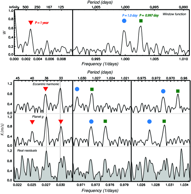
The sampling cadence of a periodic signal can alter its apparent period. An alias is a spurious periodicity generated by finite sampling of a real signal. As an extreme example, if a function of period is measured at regular intervals , it will appear constant to the observer. In the case of even sampling, the maximum frequency that can be probed without ambiguity is half the sampling frequency (the Nyquist frequency). However, this frequency cannot be unambiguously determined in the case of uneven sampling (Eyer & Bartholdi, 1999). Instead, one can identify characteristic sampling frequencies by computing the spectral window function , which depends only on the observation instants. The modulus of ranges from 0 to 1 and peaks at the sampling frequencies that cause the most severe aliases. For a real signal of frequency and a characteristic sampling frequency , aliases appear at . Figure 1 shows the window function including all the HARPS+HIRES data available for GJ 581 (M09 and V10). Optical astronomical measurements occur only at night and only during the season when the star is observable. The night time cadence introduces two sampling frequencies close to 1 day-1 (the solar and sidereal day, top right panel), and the seasonal availability generates a 1 year peak (top left panel). When the signal–to–noise is low, coherent addition of noise can produce higher power at the aliases than at the real period (see DF10). Since the announcement of the first planet candidates around GJ 581 by Bonfils et al. (2005), the yearly alias has significantly affected the determination of the orbital periods of these planets. For example, the first period proposed for the super-Earth GJ 581d was 84 days (Udry et al., 2007), a yearly alias of the currently accepted period of 67 days.
The other ingredient to the degeneracy is that the RV signal due to a planet’s Keplerian motion can be expressed as a series in powers of its orbital eccentricity, . To first order in eccentricity, a Keplerian RV signal of amplitude and period can be written as
| (1) |
where and are functions of the initial mean anomaly and the argument of the periastron, and is a constant offset that can be different for each instrument. Eqn. 1 implies that in a system with a planet of period , an additional body with period is statistically indistinguishable unless the next term in the expansion can be measured. We call the term proportional to the “first eccentric harmonic.” Due to statistical uncertainties, finite sampling, and aliasing, two planets can be misinterpreted as a single eccentric planet even when their period ratio is not exactly 2.
3 Degeneracy between planets GJ 581d and g
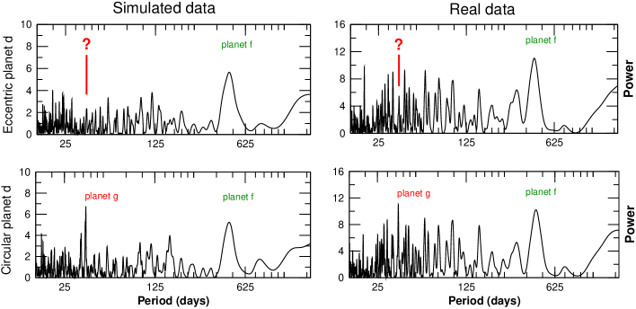
As shown by M09, the period of planet is days. Therefore, the first eccentric harmonic of this planet has a period of days ( day-1). The period of the newly found planet is days, and its aliases should appear at and days ( dayyr). Because a yearly alias of planet falls very close to the eccentric harmonic of planet , planet ’s signal will be partially absorbed by the eccentricity of planet . To illustrate this, we carry out the following experiment. We generate a synthetic dataset, the exact 6-planet solution from V10 (all circular orbits) sampled at the times of the HARPS and HIRES datasets and with Gaussian noise added (1.9 and 2.7 m/s respectively). Then, we compute the periodogram of the residuals of a 4-planet fit to this synthetic dataset (Fig. 2). Even though planet is included in the simulated data, its peak will disappear if planet is allowed to be eccentric (top left). On the other hand, planet will appear prominently if the eccentricity of planet is preliminarily fixed at 0 (bottom left). The same behavior is observed for the real data (right panels). As a general rule in modeling RV data sets, it is safer to search for significant periodicities first (i.e. preliminarily fixing the eccentricities at 0) and defer determining which model is preferred to a later stage (i.e. an eccentric planet vs. a two planet model).
In DF10, a test was developed to qualitatively assess which period is more likely in the presence of signal aliasing. The test consists of the following steps: (1) generate noiseless synthetic datasets of the signals under study, (2) compute their power spectra at the regions where the most prominent features occur (the nominal period and strongest aliases), and (3) compare them with the power spectrum of the real data (i.e. for GJ 581, the residuals to the 4-planet fit with eccentricities preliminarily fixed at 0). By power spectrum we mean the amplitude of the sinusoidal function that best fits the data at each frequency (see DF10 for further details).
We generate a synthetic dataset for each of the two candidate periods (33.5 days and 36.5 days). The bottom panels of Figure 1 show the power spectra of the real and the synthetic datasets at the nominal periods and their most prominent aliases. According to Lomb (1976), “If there is a satisfactory match between an observed spectrum and a noise-free spectrum of period , then is the true period”. While the eccentric harmonic (33.5 days) and its aliases fail to mimic the features observed in the real data (especially the daily aliases in the central panels), the candidate signal at 36.5 days does a fairly good job of reproducing most of them. Random noise modifies the power balance between peaks, so one should understand this as a first qualitative assessment. The probability of confusing planet with the eccentric harmonic of planet is quantified in Section 4.3.
4 Detailed analysis
4.1 Preliminary period search
In order to indentify promising low-amplitide periodicities, first we sequentially subtract the four most significant signals that coincide with those reported by M09 (using the systemic interface (Meschiari et al., 2009)). As discussed in Section 3, we preliminarily fix the eccentricities at 0. All parameters are refined each time a planet is added. The periodogram (Anglada-Escudé et al., 2010b) of the residuals to the 4-planet model is then computed. Both the 36.5 and 433 day signals appear prominently, see bottom right panel of Fig.2. A detection False Alarm Probability (FAP) is obtained through a Monte Carlo approach using 104 synthetic realizations of the data. Each synthetic dataset is created by scrambling the residuals to the four–planet fit, keeping the same observing epochs and instrument membership. The detection FAP is the fraction of times we obtain a signal with a higher power than the one in the real residuals. We find that both detection FAP are below 0.5%. After subtracting these two signals (36.5 and 433 days), no additional peaks are found with a detection FAP under 1%. These FAP are for detection of sinusoid–like signals only. The actual significances for the proposed new candidates are computed in the next section.
4.2 Statistical significance of GJ 581g
Recently, Gregory (2011) and Tuomi (2011) indicated that planet is not robustly confirmed when Bayesian analysis is applied. To address this issue, we consider in this section the general case where the orbits of the already-detected planets are allowed to be eccentric and compute the definitive FAP analytically using a classical Frequentist approach. Because the uncertainties in RV measurements are difficult to quantify, the statistic cannot be used to evaluate the goodness-of-fit in an absolute sense (Andrae et al., 2010). However, the can still be used in a differential way, i.e., to determine whether or not the addition of a planet is justified given the improvement of the ( are the residuals with respect to a proposed model and are the uncertainties). In this respect, we apply a version of the Fisher F-ratio test proposed by Cumming et al. (2008) that allows the addition of any number of free parameters to the null hypothesis and to the model being tested. This requires the computation of the F-ratio as
| (2) |
where and are the number of free parameters of the null hypothesis and the model to be tested respectively. The F–ratio follows an F–probability distribution with and degrees of freedom (Johnson et al., 1995). The null hypothesis includes the M09 planets (planets ) and planet , all with fully Keplerian orbits. The is obtained by adding a new planet on a 36.5 day circular orbit (requiring two extra parameters) and readjusting all the free parameters. Using the values in the two last columns of Table 1, the obtained probability of improvement-by-chance at that particular frequency is . Now one has to consider the number of independent frequencies that could also generate a spurious improvement. According to V10, M is for the HARPS+HIRES combined dataset. Therefore, the definitive FAP for planet becomes FAP(Cumming et al., 2008) and amounts to . For completeness, we add the FAP of planet () to Table 1, using the Keplerian 4-planet solution (M09) as the null hypothesis.
The F-ratio test can also be used to evaluate the significance of the eccentricity compared to a circular orbit (the null hypothesis). We find that the eccentricities of the larger amplitude planets (i.e. and ) are well-constrained but compatible with . For the low amplitude candidates ( and ), the eccentricities are unconstrained. Table 2 provides the full orbital solution.
4.3 Probability of confusion
At this point, we have assessed the FAP of the planet detection. Now we need to quantify the probability that the eccentric harmonic of planet could inflate the signal at 36.5 days by an unfortunate combination of random errors. We generate synthetic datasets by scrambling the residuals to the 6-planet fit and injecting a signal at 33.5 days (amplitude m/s). The periodogram of each dataset is then computed. We define the probability of confusion as the number of times the period of the highest peak does not lie within 1 day of the injected signal, divided by the total number of trials. For the days, we find this probability is . In % of trials, the highest peak is found near the days alias. Performing the same test by injecting the 36.5 days signal, we obtain a probability of confusion (with of trials corresponding to the 33.5 days alias). As a final check, we repeat the same experiment using random noise instead of scrambling the residuals ( 1.8 m/s for HARPS, and 3.0 m/s for HIRES). Similarly, low confusion rates ( 0.5%) are obtained. In every case, the probabilities are below , supporting the conclusion of the previous section: the probability of confusing planet with the eccentric harmonic of planet is very low. As a final check, we apply the same test using only the HARPS residuals. In more than of the trials, the highest peak is none of the injected signals, confirming that the data in M09 was not sensitive enough to distinguish between cases.
| Parameter | Four planets | Four planets | Five planets | Five planets | |
|---|---|---|---|---|---|
| M09 solution | + circular f | + circular g | |||
| Planets includedaaA planet name in parentheses indicates that this solution was used to compute the FAP of that planet. The number of free parameters is obtained as follows: 2 RV offsets (one per instrument), 5 for each Keplerian planet, and 2 for the circular orbit to be tested. | bced | bcde(f) | bcdef | bcdef(g) | |
| Eccentric orbits | 4 | 4 | 5 | 5 | |
| Circular orbits | 0 | 1 | 0 | 1 | |
| Eccentricity | |||||
| of planet | |||||
| RMS (m/s) | 2.32 | 2.21 | 2.20 | 2.10 | |
| Free parameters | 22 | 24 | 27 | 29 | |
| 241 | 241 | 241 | 241 | ||
| 707.7 | 611.8 | 602.5 | 524.8 | ||
| F ratio | 17.0 | 15.69 | |||
| FAP | 0.03% | 0.11% |
4.4 Caveats
During our analysis, we encountered a number of caveats that will require further investigation. Recent analyses by other authors using Bayesian methods (i.e. Gregory, 2011; Tuomi, 2011) seem to contradict the conclusions reached here. Thus we discuss some of these caveats and possible lines of inquiry.
Significance of spurious periodicities. We found a number of alternative periodicities for planets and that yield alternative 6-planet fits with similar significance to the solution announced by V10. Potential periods for planets and include 25.0, 26.8, 30.6, 47.8, 54.6, 59.3, 71.4, 76.4 and 97.9 days. These alternative solutions were found by computing a two-dimensional periodogram (i.e. two periodic signals are adjusted simultaneously on a grid) of the residuals of the 4-planet circular solution and refining all Keplerian parameters around the areas of lowest (Markwardt, 2009). However, a case-by-case investigation indicated that all correspond to orbital configurations with high eccentricities that suffer from several orbital crossings, making them dynamically unstable on very short timescales. To ultimately decide if such solutions were acceptable, we fixed the involved eccentricities to lower values, adjusting all other parameters in the process. The resulting orbital fits were poorer than the 6-planet solution from V10 (even assuming circular orbits for planets and ). The significance of these unphysical solutions raises the caveat that planet could be a physically-possible but spurious signal. As discussed by Tuomi (2011), Bayesian analysis methods do not yet apply down-weighting of unphysical configurations. Because such orbits have high significance, they will be oversampled, downgrading the likelihood of physically allowed orbits. This may explain the apparent contradiction of the recent Bayesian analysis with our conclusions.
Hidden planets. While planets and are detectable in both datasets, planets and are not obvious in the HIRES data alone (as also noted by V10). This indicates that some signals may be consistent with a given dataset, yet not independently detectable due to sampling issues. As a similar case, GJ 876 was a strong signal in the HIRES dataset yet undetectable with HARPS (Rivera et al., 2010). Because the completeness of on-going RV surveys can be affected as a result, this caveat requires further investigation.
Noise unknowns. We have chosen statistical tools that are as insensitive as possible to assumptions about noise: the F-ratio test and Monte Carlo scrambling of the residuals. Still, we recognize that it is not fully understood how systematic effects (e.g. stellar jitter) impact the sensitivity to low amplitude signals. A Bayesian approach with a noise parameter has been proposed to solve this problem (Tuomi, 2011). However, we think that further tests are required to assess the sensitivity of Bayesian methods in the presence of unknown systematic noise and low amplitude signals.
5 Conclusions
The eccentric harmonic of planet coincides with a yearly alias of the newly reported planet , meaning that both signals are correlated and that a premature Keplerian fit to planet prevents the detection of planet . We have found a number of unphysical solutions that fit the data just as well. Still, the proposed pair of planets and remains the only physically viable solution that significantly improves the 4-planet fit. Thus we are compelled to conclude that the presence of GJ 581 is well supported by the available data. The ultimate confirmation will require additional RV measurements and reanalysis of the data in a very convincing way. To mitigate yearly aliasing, we encourage observations at more extreme parallax factors.
We end with two cautionary notes. First, whether or not planet exists, the same cadence issues may be present in other datasets. We have found that significant periodicities in one dataset do not appear in another and that several unphysical models can appear significant. If future observations rule out the existence of planet , the fact that it passes the standard, widely-used statistical tests would bode ill for other low-amplitude planet candidates. We remark that statistical significance tests can be very sensitive to assumptions by the authors (including this work). Bayesian methods may provide stricter confidence level estimates but additional testing is required to ensure that they are not over-conservative in the low signal–to–noise regime (Jenkins & Peacock, 2011). Bayesian methods may also need to demonstrate how their conclusions are impacted by sampling issues and the inclusion of dynamical constrains in the likelihood sampling process.
Second, the eccentricity of a long period giant planet may cause spurious low amplitude signals mimicking habitable planets around Sun-like stars. Consider Jupiter as an example: its eccentric harmonic would have a period of 5.9 years (or f = 0.00046162 days-1). The corresponding yearly aliases would be at 0.0027378 days , giving candidate signals at 439 and 313 days. Complementarily, a genuine planet candidate can be missed if the eccentricity of an outer planet is adjusted prematurely. Aliasing tests on the eccentric harmonics of detected planets might be necessary in future claims of very low-amplitude signals.
Acknowledgements This work was funded by the Carnegie Fellowship Postdoctoral Program and the National Science Foundation Graduate Research Fellowship. We thank P. Butler, and S. Vogt for early access to the RV data. We thank A. Boss, J. Chanamé, J. Dunlap, D. Fabrycky, N. Haghighipour, M. Lopez-Morales, and N. Moskovitz for useful comments and discussions.
References
- Andrae et al. (2010) Andrae, R., Schulze-Hartung, T., & Melchior, P. 2010, ArXiv e-prints
- Anglada-Escudé et al. (2010a) Anglada-Escudé, G., López-Morales, M., & Chambers, J. E. 2010a, ApJ, 709, 168
- Anglada-Escudé et al. (2010b) Anglada-Escudé, G., Shkolnik, E. L., Weinberger, A. J., Thompson, I. B., Osip, D. J., & Debes, J. H. 2010b, ApJ, 711, L24
- Bonfils et al. (2005) Bonfils, X., et al. 2005, A&A, 443, L15
- Cumming et al. (2008) Cumming, A., Butler, R. P., Marcy, G. W., Vogt, S. S., Wright, J. T., & Fischer, D. A. 2008, PASP, 120, 531
- Dawson & Fabrycky (2010) Dawson, R. I., & Fabrycky, D. C. 2010, ApJ, 722, 937
- Eyer & Bartholdi (1999) Eyer, L., & Bartholdi, P. 1999, A&AS, 135, 1
- Gregory (2011) Gregory, P. C. 2011, ArXiv e-prints 1101.0800
- Heng & Vogt (2010) Heng, K., & Vogt, S. S. 2010, ArXiv e-prints 1010.4719
- Johnson et al. (1995) Johnson, N. L., Kotz, S. & Balakrishnan N. 1995, Continuous Univariate Distributions, Vol. 2. ed. Wiley (Sec. Edition, Sec. 27)
- Jenkins & Peacock (2011) Jenkins, C. R., & Peacock, J. A. 2011, MNRAS, 338
- Kasting et al. (1993) Kasting, J. F., Whitmire, D. P., & Reynolds, R. T. 1993, Icarus, 101, 108
- Lomb (1976) Lomb, N. R. 1976, Ap&SS, 39, 447
- Markwardt (2009) Markwardt, C. B. 2009, in Astronomical Society of the Pacific Conference Series, Vol. 411, Astronomical Society of the Pacific Conference Series, ed. D. A. Bohlender, D. Durand, & P. Dowler, 251–+
- Mayor et al. (2009) Mayor, M., et al. 2009, A&A, 507, 487
- Meschiari et al. (2009) Meschiari, S., Wolf, A. S., Rivera, E., Laughlin, G., Vogt, S., & Butler, P. 2009, PASP, 121, 1016
- Pepe (2010) Pepe, F. 2010, IAU Symposium : The Astrophysics of Planetary Systems. Oral Contribution
- Rivera et al. (2010) Rivera, E. J., Laughlin, G., Butler, R. P., Vogt, S. S., Haghighipour, N., & Meschiari, S. 2010, ApJ, 719, 890
- Tuomi (2011) Tuomi, M. 2011, A&A, 528, L5+
- Udry et al. (2007) Udry, S., et al. 2007, A&A, 469, L43
- Vogt et al. (2010) Vogt, S. S., Butler, R. P., Rivera, E. J., Haghighipour, N., Henry, G. W., & Williamson, M. H. 2010, ApJ, 723, 954
- von Braun et al. (2011) von Braun, K., et al. 2011, ApJ, 729, L26+
| Parameter | b | c | d | e |
|---|---|---|---|---|
| [days] | 5.368483 (10-5) | 12.91750 (0.002) | 66.845 (0.09) | 3.1485 (2 10-4) |
| 10-4(10-3)(∗) | 0.10 (0.05)(∗) | 0.11 (0.08)(∗) | 0.18 (0.08)(∗) | |
| [ms-1] | 12.49 (0.15) | 3.40 (0.18) | 1.90 (0.15) | 1.75 (0.14) |
| [deg] | 87.9 (10) | 190.6 (7) | 61.5 (8) | 104.2 (7) |
| [deg] | 190.3 (8) | 193.3 (5) | 353.9 (7) | 144.7 (5) |
| [M⊕] | 15.61 (0.16) | 5.71 (0.23) | 5.4 (0.21) | 1.805 (0.16) |
| [AU] | 0.041 | 0.073 | 0.218 | 0.028 |
| New planets (V10) | f | |||
| [days] | 440.7 (2.0) | 36.53 (0.32) | ||
| 0.17(u) | 0.19(u) | |||
| [ms-1] | 1.18 (0.13) | 1.34 (0.17) | ||
| [deg] | 330.8(u) | 68.9(u) | ||
| [deg] | 183.24 (10) | 248.1 (10) | ||
| [M⊕] | 6.28 (0.65) | 3.18 (0.4) | ||
| [AU] | 0.767 | 0.146 | ||
| [ms-1] | -2.22 (0.2) | |||
| [ms-1] | 0.934 (0.2) | |||
| 520.5 | ||||
| RMS [m/s] | 2.093 |