A Comparison of Methods for Computing Autocorrelation Time

Abstract

This paper describes four methods for estimating autocorrelation time and evaluates these methods with a test set of seven series. Fitting an autoregressive process appears to be the most accurate method of the four. An R package is provided for extending the comparison to more methods and test series.

1 Introduction

Autocorrelation time measures the convergence rate of the sample mean of a function of a stationary, geometrically ergodic Markov chain with bounded variance. Let $\{X_{i}\}_{i=1}^{n}$ be $n$ values of a scalar function of the states of such a Markov chain, where $EX_{i}=\mu$ and $\operatorname*{var}X_{i}=\sigma^{2}$. Let $\bar{X}_{n}$ be the sample mean of $(X_{1},\ldots,X_{n})$. Then, the autocorrelation time is the value of $\tau$ such that:

$$\sqrt{\frac{n}{\tau}}\cdot\frac{\bar{X}_{n}-\mu}{\sigma}\Longrightarrow N(0,1)$$ (1)

Conceptually, the autocorrelation time is the number of Markov chain transitions equivalent to a single independent draw from the distribution of $\{X_{i}\}$. It can be a useful summary of the efficiency of a Markov chain Monte Carlo (MCMC) sampler. Since there is rarely a closed-form expression for the autocorrelation time, many methods for estimating it from the data itself have been developed. This document compares four of them: computing batch means, fitting a linear regression to the log spectrum, summing an initial sequence of the sample autocorrelation function, and modeling as an autoregressive process.

For a broader context, two classic overviews of uncertainty in MCMC estimation are Geyer, (1992) and Neal, (1993, §6.3). The most popular alternative to autocorrelation time, potential scale reduction, is discussed by Gelman and Rubin, (1992).

2 Methods for computing the autocorrelation time

2.1 Batch means

Equation 1 is approximately true for any subsequence, so we can divide the $\{X_{i}\}$ into batches of size $m$ and compute the sample mean of each batch. As $m$ goes to infinity, the batch means have asymptotic variance $\sigma^{2}\cdot\tau/m$. So, if $s^{2}$ is the sample variance of $\{X_{i}\}$ and $s_{m}^{2}$ is the sample variance of the batch means, we can estimate the autocorrelation time with:

$$\hat{\tau}_{n,m}=m\frac{s_{m}^{2}}{s^{2}}$$ (2)

For this to be a consistent estimator of $\tau$, the batch size and the number of batches must go to infinity. To ensure this, I use $n^{1/3}$ batches of size $n^{2/3}$. Fishman, (1978, §5.9) discusses batch means in great detail; Neal, (1993, p. 104) and Geyer, (1992, §3.2) discuss batch means in the context of MCMC.

2.2 Fitting a linear regression to the log spectrum

In the spectrum fit method (Heidelberger and Welch,, 1981, §2.4), a linear regression is fit to the lower frequencies of the log-spectrum of the chain and used to compute an estimate of the spectrum at frequency zero, which we will denote by $\hat{I}_{0}$. Let $s^{2}$ be the sample variance of the $\{X_{i}\}$. We can estimate the autocorrelation time with:

$$\hat{\tau}=\frac{\hat{I}_{0}}{s^{2}}$$ (3)

This is implemented by the spectrum0 function in R’s CODA package (Plummer et al.,, 2006). First and second order polynomial fits are practically indistinguishable on the test series described in section 3, so this paper only explicitly includes the results for a first order fit.

2.3 Initial sequence estimators

One formula for the autocorrelation time is (Straatsma et al.,, 1986, p. 91):

$$\tau=1+2\sum_{k=1}^{\infty}\rho_{k}$$ (4)

where $\rho_{k}$ is the autocorrelation function (ACF) of the series at lag $k$. For small lags, $\rho_{k}$ can be estimated with:

$$\hat{\rho}_{k}=\frac{1}{ns^{2}}\sum_{i=1}^{n-k}(X_{i}-\bar{X}_{n})(X_{i+k}-\bar{X}_{n})$$ (5)

But, this is not defined for lags greater than $n-1$, and the partial sum $\hat{\rho}_{1}+\cdots+\hat{\rho}_{n-1}$ does not have a variance that goes to zero as $n$ goes to infinity, so substituting all values from equation 5 into equation 4 is not an acceptable way to estimate $\tau$.

Geyer, (1992) shows that, for reversible Markov chains, sums of pairs of consecutive ACF values, $\rho_{i}+\rho_{i+1}$, are always positive, so one can obtain a consistent estimator, the initial positive sequence (IPS) estimator, by truncating the sum when the sum of adjacent sample ACF values is negative.

Further, the sequence of sums of pairs is always decreasing, so one can smooth the initial positive sequence when a sum of two adjacent sample ACF values is larger than the sum of the previous pair; the resulting estimator is the initial monotone sequence (IMS) estimator. Finally, the sequence of sums of pairs is also convex. Smoothing the sum to account for this results in the initial convex sequence (ICS) estimator.

I was unable to distinguish the behavior of the IPS, IMS, and ICS estimators, so the comparisons of this paper only directly include the ICS estimator.

2.4 AR process

Another way to estimate the autocorrelation time, based on CODA’s spectrum0.ar (Plummer et al.,, 2006), is to model the series as an AR($p$) process, with $p$ chosen by AIC. We suppose a model of the form:

$$X_{t}=\mu+\pi_{1}X_{t-1}+\cdots+\pi_{p}X_{t-p}+a_{t},\qquad a_{t}\sim N(0,\sigma_{a}^{2})$$ (6)

Let $\hat{\rho}_{1:p}$ be the vector $(\hat{\rho}_{1},\ldots,\hat{\rho}_{p})$. We can obtain an estimate the AR coefficients, $\hat{\pi}_{1:p}$, with the Yule–Walker method (Wei,, 2006, pp. 136–138). Combining equations 7.1.5 and 12.2.8b of Wei, (2006, pp. 137, 274–275), we can estimate the autocorrelation time with:

$$\hat{\tau}=\frac{1-\hat{\rho}_{1:p}^{T}\hat{\pi}_{1:p}}{\left(1-1_{p}^{T}\hat{\pi}_{1:p}\right)^{2}}$$ (7)

Because the Yule–Walker method estimates the asymptotic variance of $\hat{\pi}_{1:p}$, Monte Carlo simulation can be used to generate a confidence interval for the autocorrelation time. For more information on this method, see Fishman, (1978, §5.10) and Thompson, (2010).

3 Seven test series

Figure 1: The first 10,000 elements of seven series used as a test set. See section 3 for more information.

I evaluate the methods of section 2 with seven series. The first 10,000 elements of each are plotted in figure 1.

• AR(1) is an AR(1) process with autocorrelation equal to $0.98$ and uncorrelated errors. Using equation 7, its autocorrelation time is 99. It is, in one sense, the simplest possible series with an autocorrelation time other than one.

• AR(2) is the AR(2) process with poles at $-1+0.1i$ and $-1-0.1i$:

  $$Z_{t}=1.98\,Z_{t-1}-0.99\,Z_{t-2}+a_{t},\quad a_{t}\sim N(0,1)$$ (8)

  Despite oscillating with a period of about 60, the terms in its autocorrelation function nearly cancel each other out, so its autocorrelation time is approximately two. This series is included to identify methods that cannot identify cancellation in long-range dependence.

• AR(1)-ARCH(1) is an AR(1) process with autocorrelation $0.98$ and autocorrelated errors:

  $$Z_{t}=0.98\,Z_{t-1}+a_{t},\quad a_{t}\sim N\left(0,0.01+0.99\,a_{t-1}^{2}\right)$$ (9)

  Its autocorrelation time is also 99. This series could confound methods that assume constant step variance.

• Met-Gauss is a sequence of states generated by a Metropolis sampler with Gaussian proposals sampling from a Gaussian probability distribution. It has an autocorrelation time of eight. It is a simple example of a state sequence from an MCMC sampler.

• ARMS-Bimodal is also a sequence of states from an MCMC simulation, ARMS (Gilks et al.,, 1995) applied to a mixture of two Gaussians. The sampler is badly tuned, so it rarely accepts a proposal when near the upper mode. It has an autocorrelation time of approximately 200.

• Stepout-Log-Var is a third MCMC sequence, the log-variance parameter of slice sampling with stepping out (Neal,, 2003, §4) sampling from a ten-parameter multilevel model (Gelman et al.,, 2004, pp. 138–145). Its autocorrelation time is approximately 200.

• Stepout-Var was generated by exponentiating the states of Stepout-Log-Var. Because its sample mean is dominated by large observations, its autocorrelation time, approximately 100, is not the same as that of Stepout-Log-Var. Like ARMS-Bimodal and Stepout-Log-Var, it is a challenging, real-world example of a sequence whose autocorrelation time might be unknown.

4 Comparison of methods

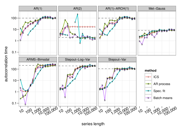
Figure 2: Autocorrelation times computed by four methods on seven series for a range of subsequence lengths. Each plot symbol represents a single estimate. The dashed line indicates the true autocorrelation time. Breaks in the lines for spectrum fit indicate instances where the method failed to produce an estimate. See section 4 for discussion.

For each series, I compare the true autocorrelation time to the autocorrelation time estimated by each method for subsequences ranging in length from 10 to 500,000. The results are plotted in figure 2. All four methods converge to the true value on all seven chains, with the exception of ICS on the AR(2) process. In general, the AR process method converges to the true autocorrelation time fastest, followed by ICS, batch means, and finally spectrum fit, which does not even produce an estimate in all cases. All four methods tend to underestimate autocorrelation times for all short sequences except those from the AR(2) process, which appears in small samples to have a longer autocorrelation time than it actually does.

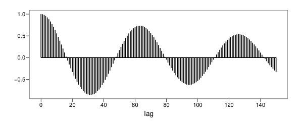
Figure 3: The autocorrelation function of the AR(2) series. See section 4 for discussion.

ICS is inconsistent on the AR(2) process because the autocorrelation function of the AR(2) process is significant at lags larger than its first zero-crossing (see figure 3). ICS and the other initial sequence estimators are not necessarily consistent when the underlying chain is not reversible; an AR(2) process is not, when considered a two state system. These estimators stop summing the sample autocorrelation function the first time its values fall below zero, so these estimators never see that values at large lags cancel values at small lags.

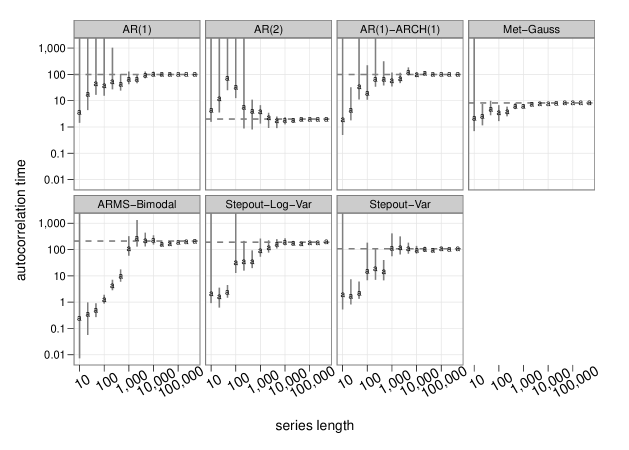
Figure 4: AR process-generated point estimates and 95% confidence intervals for the autocorrelation times of seven series for a range of subsequence lengths. The dashed line indicates the true autocorrelation time. The confidence intervals are somewhat reasonable. See section 4 for discussion.

The AR process method can also generate approximate confidence intervals for the autocorrelation time. 95% confidence intervals generated by the AR process method are shown in figure 4. The intervals are somewhat reasonable for subsequences longer than the true autocorrelation time. An exception is on AR(2), where the first few hundred elements do not represent the entire series but appear as though they might.

5 Discussion

The AR process method is more accurate than the three other methods and is the only method that, as implemented, generates confidence intervals, so I usually prefer it to the other three. The batch means estimate is faster to compute and almost as accurate, so it may be useful when speed is important and confidence intervals are not necessary.

The test set only contains seven series and reflects the type of data I encounter in my own work. To extend the comparison to other methods and series, one can use ACTCompare, an R package available at http://www.utstat.toronto.edu/mthompson.

6 Acknowledgments

I would like to thank Radford Neal for his comments on this paper and Charles Geyer for his discussion of initial sequence estimators.

References

- Fishman, (1978) Fishman, G. S. (1978). Principles of Discrete Event Simulation. John Wiley and Sons.
- Gelman et al., (2004) Gelman, A., Carlin, J. B., Stern, H. S., and Rubin, D. B. (2004). Bayesian Data Analysis, Second Edition. Chapman and Hall/CRC.
- Gelman and Rubin, (1992) Gelman, A. and Rubin, D. B. (1992). Inference from iterative simulation using multiple sequences. Statistical Science, (4):457–511.
- Geyer, (1992) Geyer, C. J. (1992). Practical Markov Chain Monte Carlo. Statistical Science, 7(4):473–511.
- Gilks et al., (1995) Gilks, W. R., Best, N. G., and Tan, K. K. C. (1995). Adaptive rejection Metropolis sampling within Gibbs sampling. Applied Statistics, 44(4):455–472.
- Heidelberger and Welch, (1981) Heidelberger, P. and Welch, P. D. (1981). A spectral method for confidence interval generation and run length control in simulations. Communications of the ACM, 24(4):233–245.
- Neal, (1993) Neal, R. M. (1993). Probabilistic inference using Markov Chain Monte Carlo methods. Technical Report CRG-TR-93-1, Dept. of Computer Science, University of Toronto.
- Neal, (2003) Neal, R. M. (2003). Slice sampling. Annals of Statistics, 31:705–767.
- Plummer et al., (2006) Plummer, M., Best, N., Cowles, K., and Vines, K. (2006). CODA: Convergence diagnosis and output analysis for MCMC. R News, 6(1):7–11.
- Straatsma et al., (1986) Straatsma, T. P., Berendsen, H. J. C., and Stam, A. J. (1986). Estimation of statistical errors in molecular simulation calculations. Molecular Physics, 57(1):89–95.
- Thompson, (2010) Thompson, M. B. (2010). Graphical comparison of MCMC performance. In preparation.
- Wei, (2006) Wei, W. W. S. (2006). Time Series Analysis: Univariate and Multivariate Methods, Second Edition. Pearson/Addison Wesley.