Non-perturbative renormalization of quark mass in $N_{f}=2+1$ QCD with the Schrödinger functional scheme

Abstract:

We present an evaluation of the quark mass renormalization factor for $N_{f}=2+1$ QCD. The Schrödinger functional scheme is employed as the intermediate scheme to carry out non-perturbative running from the low energy to deep in the high energy perturbative region. The regularization independent step scaling function of the quark mass is obtained in the continuum limit. Renormalization factors for the pseudo scalar density and the axial vector current are also evaluated for the same action and the bare couplings as two recent large scale $N_{f}=2+1$ simulations; previous work of the CP-PACS/JLQCD collaboration, which covered the up-down quark mass range heavier than $m_{\pi}\sim 500$ MeV and that of PACS-CS collaboration on the physical point using the reweighting technique.

1 Introduction

The strong coupling constant and the quark masses constitute fundamental parameters of the Standard Model. It is an important task of lattice QCD to determine these parameters using inputs at low energy scales. In the course of evaluating these fundamental parameters we need the process of renormalization in some scheme. The ${\overline{\rm MS}}$ scheme is one of the most popular schemes, and hence one would like to evaluate the running coupling constant and quark masses through input of low energy quantities on the lattice and convert them to the ${\overline{\rm MS}}$ scheme. A practical difficulty in this process is called the window problem that the conversion should be performed at much higher energy than the QCD scale. At the same time the renormalization scale $\mu$ should be kept much smaller than the lattice cut-off to reduce lattice artifacts: $1/L\ll\Lambda_{\rm QCD}\ll\mu\ll{1}/{a}$.

The Schrödinger functional (SF) scheme [1, 2] is designed to solve the window problem. A unique renormalization scale is introduced through the box size $L$ in the chiral limit and the scheme is mass independent. A wide range of renormalization scales can be covered by the step scaling function (SSF) technique. This matches our goal to obtain the coupling constant and quark masses in the $\overline{\rm MS}$ scheme. The SF scheme has been applied for evaluation of the $N_{f}=2+1$ QCD coupling [3].

For the quark mass renormalization factor the SF scheme has been applied for $N_{f}=2$ QCD [4]. At low energy scales of $\mu\sim 500$ MeV, where physical input is given, we expect the strange quark contribution to be important in addition to those of the up and down quarks. Thus the aim of this report is to go one step further and evaluate the quark mass renormalization factor in $N_{f}=2+1$ QCD . Our goal is to renormalize the bare light quark masses evaluated in two recent large-scale $N_{f}=2+1$ lattice QCD simulations [6, 7, 8] and derive the renormalization group invariant (RGI) quark mass $M$. Once the RGI mass $M$, which is scheme independent, is evaluated, the conversion into the $\overline{\rm MS}$ scheme can be carried out perturbatively.

We therefore first derive the renormalization factor $Z_{M}(g_{0})$, which converts the bare PCAC mass at a bare coupling $g_{0}$ to the RGI mass. Derivation of the renormalization factor proceeds in three steps [4, 5]

$$Z_{M}(g_{0},a/L_{\rm max})=\frac{Z_{A}(g_{0},a/L)}{Z_{P}(g_{0},a/L_{\rm max})}\frac{\overline{m}(1/L_{n})}{\overline{m}(1/L_{\rm max})}\frac{M}{\overline{m}(1/L_{n})}.$$ (1.1)

The first factor $Z_{A}/Z_{P}$ renormalizes the bare PCAC mass in the SF scheme at an appropriately low energy scale $L_{\rm max}$. The second factor ${\overline{m}(1/L_{n})}/{\overline{m}(1/L_{\rm max})}$ represents the running of the renormalized mass from $L_{\rm max}$ to a high energy scale $L_{n}$, which is evaluated non-perturbatively in the SF scheme. The last factor ${M}/{\overline{m}(1/L_{n})}$ represents the running from $L_{n}$ to infinitely high energy scale and is evaluated perturbatively for an appropriately high energy scale $L_{n}$.

2 Step scaling function

We adopt the renormalization group improved Iwasaki gauge action and the non-perturbatively ${O}(a)$ improved Wilson fermion action with the clover term. The Dirichlet boundary condition for the spatial gauge link is set to

$$U_{k}(x)|_{x_{0}=0}=U_{k}(x)|_{x_{0}=T}=1$$ (2.1)

and the twisted periodic boundary condition of the fermion fields in the three spatial directions is

$$\psi(x+L\hat{k})=e^{i\theta}\psi(x),\quad{\overline{\psi}}(x+L\hat{k})=e^{-i\theta}{\overline{\psi}}(x),\quad\theta=0.5.$$ (2.2)

We prepare seven renormalized coupling values to cover weak to strong coupling regions [3]. For each coupling we use three box sizes $L/a=4,6,8$ to take the continuum limit. At the three lattice sizes the values of $\beta$ and $\kappa$ were tuned to reproduce the same renormalized coupling keeping the PCAC mass to zero. On the same parameters we evaluate the pseudo scalar density renormalization factor ${Z_{P}(g_{0},a/L)}$ and ${Z_{P}(g_{0},a/(2L))}$ at two box sizes.

The renormalization factor $Z_{P}$ is defined in terms of two-point functions [4] of pseudo scalar density at bulk and at boundary. Taking the ratio of two renormalization factors at two renormalization scales $\mu=1/L$ and $1/(2L)$ we get the step scaling function (SSF) on the lattice

$$\Sigma_{P}\left(u,\frac{a}{L}\right)=\left.\frac{Z_{P}(g_{0},a/(2L))}{Z_{P}(g_{0},a/L)}\right|_{\overline{g}^{2}(L)=u,m=0},$$ (2.3)

where mass independent scheme in the massless limit is adopted.

We perform a perturbative improvement of the SSF before taking the continuum limit. For this purpose we need a perturbative evaluation of the lattice artifact in the SSF

$$\delta_{P}(u,a/L)=\frac{\Sigma_{P}\left(u,{a}/{L}\right)-\sigma_{P}(u)}{\sigma_{P}(u)}.$$ (2.4)

Instead of calculating $\delta_{P}$ at one and two-loop level perturbatively we calculate SSF’s directly by Monte-Carlo simulations at very weak coupling $\beta\geq 10$. The artifact is fitted to a polynomial form for each $a/L$,

$$1+\delta_{P}(u,a/L)=1+d_{1}(a/L)u+d_{2}(a/L)u^{2}.$$ (2.5)

Since the quadratic fit provides a reasonable description of data [5] we opt to cancel the $O(a)$ contribution dividing out the SSF by the quadratic fit.

Scaling behavior of the improved SSF is plotted in the left panel of Fig. 1.

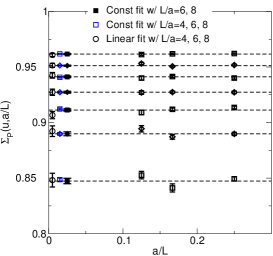
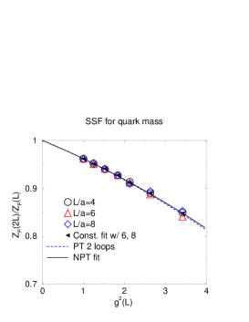
Figure 1: The SSF on the lattice with its continuum extrapolation at each renormalization scale (left) and the RG flow of the SSF (right).

Almost no scaling violation is found. We performed three types of continuum extrapolation: a constant extrapolation with the finest two (filled symbols) or all three data points (open symbols), or a linear extrapolation with all three data points (open circles), which are consistent with each other. The constant fit was employed with the finest two data points to find our continuum value.

The RG running of the continuum SSF is plotted in the right panel of Fig. 1. A polynomial fit of the continuum SSF to third order yields

$$\sigma_{P}(u)=1+p_{0}u+p_{1}u^{2}+p_{2}u^{3},$$ (2.6)

$$p_{1}=-0.002826,\quad p_{2}=0.000031$$ (2.7)

fixing the first coefficients $p_{0}$ to its perturbative value. The fitting function is also plotted (solid line) together with the two loops perturbative running (dashed line).

Multiplying the SSF according to a sequence of couplings $u_{i}$, which differ by a factor two in the renormalization scale, starting from $u_{0}=\overline{g}^{2}(L_{\rm max})$ we get the non-perturbative running of mass

$${\prod_{i=1}^{n}\sigma_{P}(u_{i})}=\frac{\overline{m}(1/L_{n})}{\overline{m}(1/L_{\rm max})}.$$ (2.8)

In Fig. 2 we plot the non-perturbative running mass $\overline{m}(1/L_{n})/M$ in units of the RGI mass as a function of the scale $\mu/\Lambda_{\rm SF}$, where $\mu=1/L_{n}$.

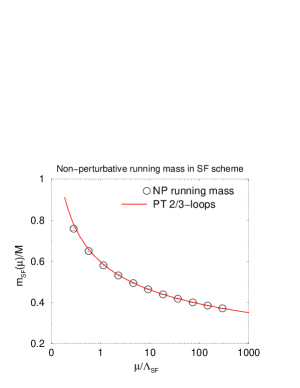
Figure 2: The non-perturbative running mass in the SF scheme. Solid line is a perturbative running with two and three loops RG function for the mass and the coupling.

3 $Z_{P}$ and $Z_{A}$ at low energy scale

We evaluate the renormalization factor $Z_{P}$ at the same bare coupling $\beta$, $1.83$, $1.90$ and $2.05$ adopted in the large scale simulations [6, 7, 8]. The reference scale $L_{\rm max}$ is given by the box size we used in this evaluation. The renormalized coupling $\overline{g}^{2}(L_{\rm max})$ should not exceed our maximal value $5.13$ for the coupling SSF significantly. We use the box size of $L/a=4$ for $\beta=1.83$ and $1.90$ to define $L_{\rm max}$ and $L/a=6$ for $\beta=2.05$. We adopt the lattice spacing $a$ as an intermediate scale.

The remaining ingredient of the renormalization factor (1.1) at low energy is $Z_{A}$ of the axial vector current. We calculate the renormalization factor according to the procedure in Ref. [9] through the axial Ward-Takahashi identity, which is applicable to small non-vanishing PCAC mass. The box size $L$ for the axial current need not coincide with $L_{\rm max}$ since $Z_{A}$ is scale independent in the continuum limit.

In this paper we adopted the following box size at each $\beta$ to define $Z_{A}$: $12^{3}\times 30$, $\theta=0.5$ at $\beta=1.83$, $10^{3}\times 24$, $\theta=0$ at $\beta=1.90$ and $12^{3}\times 30$, $\theta=0.5$ for $\beta=2.05$. The disconnected contribution [9] is included. In the left panel of Fig. 3 we plot the values for $Z_{A}$ according to our definition (filled circles), together with those without the disconnected contribution (open symbols). Scattering of points starting around $\beta=1.95$ indicates that lattice artifacts are increasingly large in our data for large lattice spacings.

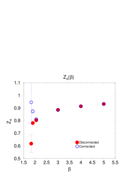
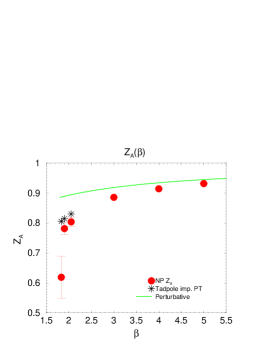
Figure 3: $\beta$ dependence of $Z_{A}(g_{0})$ with and without disconnected diagrams (left) and comparison with perturbative results (right).

In the right panel of Fig. 3 we compare our $Z_{A}(g_{0})$ with perturbative behavior (solid line) and results from the tadpole improved perturbation theory (star symbols).

4 RGI mass renormalization factor

We derive the renormalization factor $Z_{M}$ for the RGI mass, which is intended to renormalize the bare PCAC masses obtained in the two large scale simulations. The three hadron masses, $m_{\pi}$, $m_{K}$, $m_{\Omega}$ were used in Ref. [7, 8] to determine the light quark masses and the lattice spacing. Two choices $m_{\pi}$, $m_{\rho}$ $m_{K}$ or $m_{\pi}$, $m_{\rho}$ $m_{\phi}$ were adopted in Ref. [6]. The results for $Z_{M}$ are listed in Table 1. Also listed are the renormalization factors $Z_{m}^{\overline{\rm MS}}(\beta,\mu=2\ {\rm GeV})$ in the $\overline{\rm MS}$ scheme at a renormalization scale $\mu=2$ GeV. We emphasize that the renormalization factor here is defined in terms of the renormalization group functions for three flavors.

$\beta$	$Z_{M}$	$Z_{m}^{\overline{\rm MS}}$ ($K$)	PT(tad) $Z_{m}^{\overline{\rm MS}}$ ($K$)	$Z_{m}^{\overline{\rm MS}}$ ($\phi$)	PT(tad) $Z_{m}^{\overline{\rm MS}}$ ($\phi$)
$1.83$ [6]	$1.33(15)$	$1.04(12)$	$1.07161$	$1.04(12)$	$1.07019$
$1.90$ [6]	$1.693(46)$	$1.315(35)$	$1.09973$	$1.315(35)$	$1.09955$
$2.05$ [6]	$1.862(41)$	$1.417(29)$	$1.14487$	$1.416(29)$	$1.1446$
$1.90$ [7]	$1.693(46)$	$1.344(36)$	$1.11322$
$1.90$ [8]	$1.693(46)$	$1.347(36)$	$1.11322$

Table 1: $Z_{M}$ for the RGI mass and $Z_{m}^{\overline{\rm MS}}(2\ {\rm GeV})$ in the $\overline{\rm MS}$ scheme. ($K$) or ($\phi$) means which meson mass is used for physical scale input. Perturbative results with tadpole improvement are also listed.

The error in the renormalization factor includes all the statistical and systematic ones except for that from the choice of the reference scale $L_{\rm max}$. We tried a rough estimate of ${O}((a/L_{\rm max})^{2})$ error and we find a few percent effect at $\beta=2.05$, while the magnitude may increase to a 10 % level at lower values of $\beta$. However, a firmer conclusion requires the step scaling function at the couplings stronger than those explored in the present work.

As the last step we apply our renormalization factor to the bare PCAC masses in Refs. [6, 7, 8] to obtain values for the renormalized quark masses. We notice that the chiral perturbation theory was used to extract the physical quark mass in Ref. [6, 7], while the reweighting technique was adopted in Ref. [8] to evaluate the quark mass directly on the physical point. The numerical results are given in Table 2 and are plotted in Fig. 4 both for the averaged up and down quark mass (left panel) and for the strange quark mass (right panel). For the old CP-PACS/JLQCD work of Ref. [6] results with $K$ and $\phi$ meson input are plotted (filled squares and circles) together with perturbatively renormalized masses using tadpole improved renormalization factor (open squares and circles). The upward triangle represents the result for the more recent work of PACS-CS evaluated directly on the physical point using the reweighting technique [8]. The downward triangle represent a result of chiral extrapolation from the simulation point reaching down to $m_{\pi}=155$ MeV [7].

$\beta$	$M_{ud}^{\rm RGI}$	$m_{ud}^{\overline{\rm MS}}$	$M_{s}^{\rm RGI}$	$m_{s}^{\overline{\rm MS}}$
$1.83$ [6]	$3.30(38)$	$2.59(30)$	$86(10)$	$67.7(7.9)$
$1.90$ [6]	$4.47(17)$	$3.47(13)$	$115.3(4.4)$	$89.5(3.4)$
$2.05$ [6]	$5.29(24)$	$4.02(18)$	$136.1(6.5)$	$103.6(4.9)$
$1.90$ [7]	$3.84(16)$	$3.05(12)$	$110.5(4.0)$	$87.7(3.1)$
$1.90$ [8]	$3.49(34)$	$2.78(27)$	$109.0(3.0)$	$86.7(2.3)$

Table 2: Non-perturbatively renormalized mass for the averaged up and down quark and for the strange quark. $M^{\rm RGI}$ is the RGI mass and $m^{\overline{\rm MS}}$ is that in the $\overline{\rm MS}$ scheme at a scale $\mu=2$ GeV. The unit is in MeV. $K$-meson mass is used for physical input.

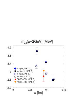
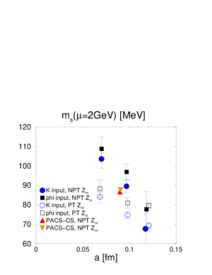
Figure 4: Scaling behavior of $m_{ud}^{\overline{\rm MS}}$ (left) and $m_{s}^{\overline{\rm MS}}$ (right).

It is disappointing that the old CP-PACS/JLQCD results do not exhibit a better scaling behavior by going from perturbative to non-perturbative renormalization factor. However, we should note a significant change in the average up and down quark mass with the recent PACS-CS work (filled triangles). This represents a systematic error due to chiral extrapolation of the old CP-PACS/JLQCD work whose pion mass reached only $m_{\pi}\sim 500$ MeV. We should also note that the renormalization factor $Z_{A}$ involves a large uncertainty at $\beta=1.83$ which is not reflected in the error bar of Fig. 4. We feel that results at $\beta=2.05$ using simulation with physical pion mass are needed to find the convincing values for light quark masses with our approach.

5 Conclusion

We have presented a calculation of the quark mass renormalization factor for the $N_{f}=2+1$ QCD in the mass independent Schrödinger functional scheme in the chiral limit. We calculate the SSF of the running mass on the lattice and applied a perturbative improvement. We find that the step scaling function shows a good scaling behavior and the continuum limit may be taken safely with a constant extrapolation. The non-perturbative SSF turned out to be almost consistent with the perturbative two loops result. We then derive the renormalization factor of the pseudo scalar density at low energy and that of axial vector current. Multiplying these factors we evaluate the non-perturbative renormalization factors for the RGI mass and that in the $\overline{\rm MS}$ scheme at a scale $\mu=2$ GeV.

Applying our non-perturbative renormalization factor to the present PACS-CS simulation result evaluated directly at the physical point yields $m_{ud}^{\overline{\rm MS}}(\mu=2\ {\rm GeV})=2.78(27)$ MeV for the average up and down quark, and $m_{s}^{\overline{\rm MS}}(\mu=2\ {\rm GeV})=86.7(2.3)$ MeV for the strange quark. Simulations at weaker couplings under way will tell if these values stay toward the continuum limit.

This work is supported in part by Grants-in-Aid of the Ministry of Education (Nos. 10143538, 20105001, 20105002, 20105003, 20105005, 20340047, 20540248, 20740139, 21340049, 22105501, 22244018, 22740138).

References

- [1] M. Lüscher, R. Narayanan, P. Weisz and U. Wolff, Nucl. Phys. B 384 (1992) 168.
- [2] S. Sint, Nucl. Phys. Proc. Suppl. 94 (2001) 79 and references there in.
- [3] S. Aoki et al. [PACS-CS Collaboration], JHEP 10 (2009) 053.
- [4] M. Della Morte, R. Hoffmann, F. Knechtli, J. Rolf, R. Sommer, I. Wetzorke and U. Wolff [ALPHA Collaboration], Nucl. Phys. B 729 (2005) 117.
- [5] S. Aoki et al. [PACS-CS collaboration], JHEP 1008 (2010) 101.
- [6] T. Ishikawa et al. [JLQCD Collaboration], Phys. Rev. D 78 (2008) 011502.
- [7] S. Aoki et al. [PACS-CS Collaboration], Phys. Rev. D 79 (2009) 034503.
- [8] S. Aoki et al. [PACS-CS Collaboration], Phys. Rev. D 81 (2010) 074503.
- [9] M. Della Morte, R. Hoffmann, F. Knechtli, R. Sommer and U. Wolff, JHEP 0507 (2005) 007.