Entanglement transitions in random definite particle states

Abstract

Entanglement within qubits are studied for the subspace of definite particle states or definite number of up spins. A transition from an algebraic decay of entanglement within two qubits with the total number $N$ of qubits, to an exponential one when the number of particles is increased from two to three is studied in detail. In particular the probability that the concurrence is non-zero is calculated using statistical methods and shown to agree with numerical simulations. Further entanglement within a block of $m$ qubits is studied using the log-negativity measure which indicates that a transition from algebraic to exponential decay occurs when the number of particles exceeds $m$. Several algebraic exponents for the decay of the log-negativity are analytically calculated. The transition is shown to be possibly connected with the changes in the density of states of the reduced density matrix, which has a divergence at the zero eigenvalue when the entanglement decays algebraically.

I Introduction

Entanglement has been extensively investigated in the recent past, as it is a critical resource for quantum information processing  Nielsen and Chuang (2000). One model of quantum computation, the one-way quantum computer Raussendorf and Briegel (2001), relies explicitly on entanglement. The resource of entanglement is not at all rare, a random pure quantum state is typically highly entangled Bandyopadhyay and Lakshminarayan (2002); Hayden et al. (2006). In fact there is so much entanglement in typical random pure states that recent studies Bremner et al. (2009); Gross et al. (2009) find them not to be useful for one-way quantum computation. This motivates the question of studying subsets of states with a control over the amount of entanglement available.

It is well known that most of the entanglement in many body quantum systems is multipartite. In random pure states of $N$ qubits, we need to consider blocks whose total size is at least larger than $N/2$, for them to be entangled Kendon et al. (2002). This being the case, entanglement in smaller blocks is nearly impossible to observe. Previous studies have shown how rare it is to have two qubits entangled in a many qubit random pure state Scott and Caves (2003); Kendon et al. (2002). In this paper it is shown that there is a surprising connection between the number of up-spins or particles present in definite particle states and entanglement. Thus producing definite particle random states, as defined below, may allow control over the type of entanglement that is desired. For instance if two qubit entanglement is to be obtained, it is shown that typical three-particle states will render this nearly impossible to achieve. The border between probable and improbable is described by a transition from an algebraic to an exponential decay, which is typically obtained at phase transitions. Further, the approach presented in this paper might shed light on methods that are applicable to a wider class of problems in the area of quantum complex systems.

Random pure states, or “full” random pure states, belong to the ensemble of states that are uniformly sampled from the Hilbert space, with the only constraint being normalization, in other words sampled from the unique Haar measure. Such states arise for instance in mesoscopic systems Beenakker (1997), nuclear physics Brody et al. (1981) etc. and have been modeled as eigenfunctions of random matrices from the usual Gaussian ensembles Mehta (2004). There have been studies that explore how to efficiently produce operators with statistical properties of random matrices Emerson et al. (2003). Classically chaotic systems have long been known to exhibit such states in their quantum limit, and studies of entanglement in quantum chaotic systems often take recourse to random states Benenti (2009); Lakshminarayan (2001).

The ensemble of interest in this work is taken to be the one where all the vectors that are constrained to be in the definite particle subspace are equally likely, subject again only to the constraint of normalization. This is equivalent to assuming that the Hamiltonian in the definite particle symmetry reduced subspaces are full random matrices. In this paper the random matrices are taken to be of the GOE (Gaussian Orthogonal Ensemble) Mehta (2004) type and hence the states studied are real. Any study that uses random states or random matrices is justified as a baseline with which to compare realistic Hamiltonian systems that may involve interactions in a complex, nonintegrable manner. In particular it is possible that due to the few-body nature of typical interactions, ensembles such as the Embedded GOE Kota (2001) will be of interest. However we believe that studying a usual ensemble like the GOE will form a baseline for entanglement studies of a rather large class of physically important systems which conserve particle number, or total spin.

A definite particle state is a random pure state in a fixed $S_{z}$ subspace formed by the basis vectors of the Hilbert space, which, when expressed in the spin-$z$ basis, have a fixed number, say $l$, of “ones”, or spin ups. Clearly many Hamiltonian systems including spin models such as the quantum spin-glass Georges et al. (2000), or the disordered Heisenberg chains Brown et al. (2008) are potential places where such states can occur as eigenstates. The number of particles allows to add complexity to the states in a systematic manner, and interesting properties for entanglement unfold in the process. Studies of entanglement in two-electron systems for instance are found in Naudts and Verhulst (2007). One other class of problems where there is potential to see the kind of transitions noted in this paper is in the study of site-entanglement of fermions in a lattice Larsson and Johannesson (2006), where the total number of qubits of this paper will be translated to the total number of sites, the number of particles will be the number of fermions and the block will refer to the sites within which the entanglement is found. It may also be noted that translationally invariant definite particle states with highly entangled nearest neighbor were constructed as “entangled rings” O’Connor and Wootters (2001).

A previous study of entanglement in random one-particle states showed that the averaged concurrence between any two qubits scales as $1/N$ Lakshminarayan and Subrahmanyam (2003). Thus with increasing number of qubits entanglement between any two still remains considerable, although decreasing, in contrast to a full random state. In this paper it is shown that for random two-particle states the average entanglement between two qubits scales as $1/N^{2}$, while for three-particle states this becomes exponentially small, as it goes as $\exp(-N\ln(N))$. Thus when the number of particles exceeds two a transition is seen in the entanglement between two qubits. It maybe noted that for full random states it is not precisely known how such an entanglement scales with the number of qubits.

It is possible to generalize the results of concurrence between two qubits to entanglement within the block $A$ having $m$ qubits of the system for instance by studying the log-negativity measure Vidal and Werner (2002). Numerical and some analytical evidence points to the plausible result that the entanglement decays with $N$ algebraically if the number of particles in the subspace ($l$) is less than or equal to the block-length ($m$). Once again the decay of entanglement becomes exponential when the number of particles exceeds the block-length. A study of the density of states of the reduced density matrix also shows a transition when the number of particles exceeds the block size; namely a divergence at the zero eigenvalue is replaced by a vanishing density. This paper studies this divergence and how this impacts the partial transpose in such a way that entanglement undergoes the kind of transition that is discussed herein.

The structure of the paper is as follows. In section  II, details of definite particle states and reduced density matrices of blocks of qubits are given. In section  III the entanglement between two qubits is studied as a function of the number of particles present in the state and as a function of the total number of qubits. Detailed analytical results are derived utilizing concurrence as a measure of entanglement. To demonstrate that the transition is independent of the particular measure of entanglement, as well as to facilitate generalization to larger blocks, the log-negativity between two qubits is also considered here. In section  IV entanglement among larger sets of qubits is studied by means of log-negativity and a few analytical and several numerical results are presented. In section V the density of states of the density matrix is studied and it is shown that there is a transition in its character as the number of particles exceeds the block size. Evidence is presented that this results in, or is reflected as, the entanglement transition.

II Definite particle states

A definite $l$-particle state is best written by grouping states with a given number of particles present in one block, say $A$, and its complementary block, say $B$. Let the number of qubits in block $A$ be $m$ and let $l\geq m$. Label the states by the number of particles (or total spin $S_{z}$) in subsets $A$ and $B$ to write:

$$|\psi\rangle = \sum_{j=1}^{{N-m\choose l}}c_{1j}^{(0)}|0\rangle_{A}|l\rangle^{j}_{B}+\sum_{j=1}^{{N-m\choose l-1}}\sum_{i=1}^{{m\choose 1}}c_{ij}^{(1)}|1\rangle_{A}^{i}|l-1\rangle_{B}^{j}$$ (1)

$$+ \ldots+\sum_{j=1}^{{N-m\choose l-m}}c_{1j}^{(m)}|m\rangle_{A}|l-m\rangle_{B}^{j}.$$

The reduced density matrix of the subsystem $A$ denoted $\rho_{A}$, is the state of the block of qubits we are interested in studying. These blocks correspond to having a given number of particles, $k$, in the subsystem $A$ and can be identified with one of the terms in the expression for the state. Further, each of these blocks can be written as $G_{k}=Q_{k}Q_{k}^{\dagger}$ where $Q_{k}$ is a matrix whose entries are the coefficients $c_{ij}^{(k)}$ of the state. The dimensions (#rows $\times$ #columns) of, the in general rectangular matrices, $Q_{k}$ and the square matrices $G_{k}$ are given by

$$\mbox{dim}\;Q_{k}={m\choose k}\times{N-m\choose l-k},\;\;\mbox{dim}\;G_{k}={m\choose k}\times{m\choose k}.$$ (2)

The condition that the trace of a density matrix is unity implies that $\sum_{k}{\rm Tr}(Q_{k}Q_{k}^{\dagger})=1.$ To construct the ensemble of $l$-particle states, draw all the $\mathcal{N}={N\choose l}$ coefficients $c_{ij}^{(k)}$ from the normal distribution $N(0,1)$ and normalize them so that the trace condition is met. This is equivalent to choosing them uniformly with the only constraint being normalization Wootters (1990).

The case when the number of particles $l$ is less than the block length $m$ can be similarly written:

$$|\psi\rangle = \sum_{j=1}^{{N-m\choose l}}c_{1j}^{(0)}|0\rangle_{A}|l\rangle^{j}_{B}+\sum_{j=1}^{{N-m\choose l-1}}\sum_{i=1}^{{m\choose 1}}c_{ij}^{(1)}|1\rangle_{A}^{i}|l-1\rangle_{B}^{j}$$ (3)

$$+ \ldots+\sum_{i=1}^{{m\choose l}}c_{i1}^{(l)}|l\rangle_{A}^{i}|0\rangle_{B}.$$

In this case the last non-zero block has dimension ${m\choose l}$, however it has only one non-zero eigenvalue, as the corresponding density matrix $Q_{l}Q_{l}^{\dagger}$ is that of a unnormalized pure state. The sum of the dimensionality of the $G_{k}$ block matrices in this case is less than $2^{m}$ and hence there are exact zero eigenvalues, in other words, the density matrix is rank-deficient. For example in the simple case of one-particle states, the two qubit density matrix has one exact zero eigenvalue. In fact it is easy to see that in general for one-particle states, the number of non-zero eigenvalues of the reduced density matrix of any number of qubits is at most two. From the dimension of the $Q_{k}$ matrices above we can formally write the minimum number of exact zero eigenvalues of the reduced density matrix for the case when $l<m$. Written in terms of rank:

$$\mbox{rank}\;\rho_{A}\leq\sum_{k=0}^{l}\mbox{min}\;\left[{m\choose k},\,{N-m\choose l-k}\right]<2^{m}.$$ (4)

In the case of $l\geq m$ the rank of typical reduced density matrices is full, that is the rank is $2^{m}$. This is seen by examining the dimensions of each of the blocks $G_{k}$. From Eq. (2) it follows that typical $G_{k}$ will not have exact zero eigenvalues if

$${m\choose k}\leq{N-m\choose l-k}.$$ (5)

A straightforward but nontrivial calculation shows that this is always the case if $N\geq 2l$. The equality is possible only when $l=m$. It is indeed assumed that $N\geq 2l$ throughout this paper without any loss of generality, due to the particle-hole symmetry. In the special case of $N=2l$ and $l=m$ all of the $Q_{k}$ matrices are of square type and the $G_{k}$ are formed then from symmetric states. This has implications for the density of states as will be discussed later in this paper (see section  V). With these details about the structure of the reduced density matrices of definite particle states, we now turn to a study of entanglement in them.

III Entanglement between two qubits in a definite particle state

The reduced density matrix of a block $A$ with $m=2$ qubits in a pure state of $l\geq 2$ particles with the total number of qubits equal to $N$ can be written as:

$$\rho_{A}=\left(\begin{matrix}a_{00}&0&0&0\\ 0&a_{11}&a_{12}&0\\ 0&a_{12}^{*}&a_{22}&0\\ 0&0&0&a_{33}\\ \end{matrix}\right),$$ (6)

where, $a_{00}=\sum_{i=1}^{\mu_{0}}(c_{1i}^{(0)})^{2},\;\;\;a_{33}=\sum_{i=1}^{\mu_{2}}(c_{1i}^{(2)})^{2}$, and

$$\left(\begin{matrix}a_{11}&a_{12}\\ a_{12}^{*}&a_{22}\\ \end{matrix}\right)=Q_{1}Q_{1}^{\dagger},\;Q_{1}=\left(\begin{matrix}c_{11}^{(1)}&\ldots&c_{1\mu_{1}}^{(1)}\\ c_{21}^{(1)}&\ldots&c_{2\mu_{2}}^{(1)}\\ \end{matrix}\right).$$ (7)

Here $\mu_{i}={N-2\choose l-i},\;i=0,1,2$. The results presented in this work deal with real coefficients, ${c_{ij}^{(k)}}^{*}=c_{ij}^{(k)}$, a situation that would be relevant for example for systems with time reversal symmetry. The central features, including the scaling, remain the same in the complex case. Also note that while the above expressions have been written when $l\geq 2$, it is straightforward to write the same when $l=1$, the case of 1-particle states. As a previous work has dealt with 1-particle states Lakshminarayan and Subrahmanyam (2003), this is not considered further, however a detailed analysis of log-negativity in this case is presented later on in this paper.

III.1 Concurrence between two qubits

Concurrence Wootters (1998) is a measure of entanglement present between two qubits such as those in the subsystem $A$. The above structure in Eq. (6), greatly simplifies the expression for concurrence O’Connor and Wootters (2001)

$$C=2\;\mbox{max}(|a_{12}|-\sqrt{a_{00}a_{33}},0),$$ (8)

and this allows for analytical estimates to be made, in contrast to the case of a full random state. Due to the large number of coefficients $c_{ij}^{(k)}$ involved, it is a good approximation to assume that the normalization constraint is only important to set their scale and that they are otherwise independent. This implies that these are i.i.d. random variables drawn from the normal distribution $N(0,1/\mathcal{N})$; recall that $\mathcal{N}={N\choose l}$. The random numbers are ingredients for the random variables $a_{00}$, $a_{12}$ and $a_{33}$ that determine the concurrence and hence the entanglement.

The approach to finding the mean concurrence will be to first estimate the probability that it will be nonzero. The term $a_{12}$ involves a correlation between two strings of normally distributed numbers, each of length $\mu_{1}$, the two rows of the matrix $Q_{1}$ in Eq. (7). On the other hand $a_{00}$ maybe taken to be effectively its average and considered to be non-fluctuating, as it is a sum over $\sim N^{l}$ random terms. The following approximation then ensues:

$$\mbox{Pr}(C>0)\approx\mbox{Pr}(|a_{12}|-\sqrt{\langle a_{00}\rangle}\sqrt{a_{33}}>0).$$ (9)

The distribution of $|a_{12}|$, $P_{12}$, is of central importance and can obtained from, for example, from the probability density function of one of the marginals of the Wishart distribution for correlation matrices Wishart (1928). Suppressing the calculation, the result is

$$P_{12}\left(|a_{12}|=x\right)=2\mathcal{N}\frac{K_{\nu}(\mathcal{N}x)}{\sqrt{\pi}\Gamma(\mu_{1}/2)}\left(\frac{\mathcal{N}x}{2}\right)^{\nu},$$ (10)

where $K_{\nu}(x)$ is the modified Bessel function of the second kind, and $\nu=(\mu_{1}-1)/2$. The distribution of $\sqrt{a_{33}}$, $P_{33}$, follows from that of (square root of) a chi-squared distribution with $\mu_{2}$ degrees of freedom:

$$P_{33}\left(\sqrt{a_{33}}=y\right)=\dfrac{\mathcal{N}^{\mu_{2}/2}}{2^{\mu_{2}/2-1}\Gamma(\mu_{2}/2)}y^{\mu_{2}-1}e^{-\mathcal{N}y^{2}/2}.$$ (11)

Thus in view of the approximation above it follows that:

$$\mbox{Pr}(C>0)=\int_{0}^{\infty}P_{33}(y)\int_{\sqrt{\langle a_{00}\rangle}y}^{\infty}P_{12}(x)\,dx\,dy.$$ (12)

This can be evaluated by steps which are outlined here: (a) change variable $y$ to $\sqrt{2y/\mathcal{N}}$, and $\mathcal{N}x$ to $x$; (b) use the integral representation $K_{\nu}(x)=\int_{0}^{\infty}e^{-x\cosh t}\cosh(\nu t)\,dt$, and change variable from $x\cosh t$ to $x$. This leads to the exact expression (given the approximation in Eq. (9))

$$\mbox{Pr}(C>0)=\beta\int_{0}^{\infty}\dfrac{\cosh(\nu t)}{\cosh^{\nu+1}t}\int_{0}^{\infty}y^{\frac{\mu_{2}}{2}-1}e^{-y}\,\Gamma\left(\nu+1,\sqrt{\gamma y}\cosh t\right)\,dy\,dt.$$ (13)

Here $\beta=2^{-\nu+1}/\sqrt{\pi}\Gamma(\mu_{1}/2)\Gamma(\mu_{2}/2)$, and $\gamma=2\langle a_{00}\rangle\mathcal{N}$. While further simplification is possible, for example by expanding $e^{-y}$, it is expedient to seek a non-trivial upper bound that reveals the nature of the decay with $N$, the number of qubits. A careful examination of the integrands indicate that this can be most easily achieved by using $e^{-y}<1$ and thus effectively removing the exponential from the integral. The remaining integrals can be done exactly to give the first inequality below, while the second follows from standard inequalities for ratios of gamma functions:

$$\mbox{Pr}(C>0)<\dfrac{2^{\mu_{2}}}{\gamma^{\mu_{2}/2}\sqrt{\pi}}\dfrac{\Gamma\left(\frac{\mu_{1}+\mu_{2}}{2}\right)}{\Gamma\left(\frac{\mu_{1}}{2}\right)}\dfrac{\Gamma(\frac{\mu_{2}+1}{2})}{\Gamma(\frac{\mu_{2}}{2}+1)}\\ <\frac{1}{\sqrt{\pi}}\left(\dfrac{2\mu_{1}\eta}{\gamma}\right)^{\frac{\mu_{2}}{2}}\dfrac{1}{\sqrt{\frac{\mu_{2}}{2}+\frac{1}{4}}},$$ (14)

where $\eta=1+(\mu_{2}-2)/(2\mu_{1})$. Note that when the number of particles is much less than the number of qubits, $\eta\approx 1$. For the case of two particle states, $l=2$, the first inequality yields

$$\mbox{Pr}(C>0)<\frac{2\sqrt{2}}{\pi}\frac{1}{\sqrt{N}},$$ (15)

as $\mu_{1}=N-2$ and $\mu_{2}=1$. The inequality is valid for large $N$, especially as the value of $\langle a_{00}\rangle$ is taken to be 1. As a matter of fact that this is an excellent estimate by itself is seen in Fig. (1).

The two particle case is of special interest and can be essentially derived from simpler formulae, if it is observed that the fluctuations in $a_{33}$, arising from a single realization of the random variables, is more than the others. Note that: $a_{00}\sim\mu_{0}/\mathcal{N}\sim 1$, $a_{33}\sim\mu_{2}/\mathcal{N}\sim 1/N^{2}$, and $|a_{12}|^{2}\sim\mu_{1}/\mathcal{N}^{2}\sim 4/N^{3}$. Hence typically the concurrence will indeed be zero. Replacing the average values for the fluctuating $a_{00}$ and $|a_{12}|$ results in $\mbox{Pr}(C>0)\approx\mbox{Pr}(\sqrt{a_{33}}<\sqrt{\frac{2}{\pi}}\frac{2}{N^{3/2}})=\frac{2\sqrt{2}}{\pi}\frac{1}{\sqrt{N}},$ coinciding with the upper bound just derived.The average value of $|a_{12}|$ is used, rather than the (square root of the) average of $|a_{12}|^{2}$; the exact distribution can be used to show that $\langle|a_{12}|^{2}\rangle=\frac{\pi}{2}(\langle|a_{12}|\rangle^{2})$. Thus for two particle states the probability of concurrence being positive decreases algebraically, in contrast to the one-particle case when $P(C>0)=1$, as $a_{33}=0$.

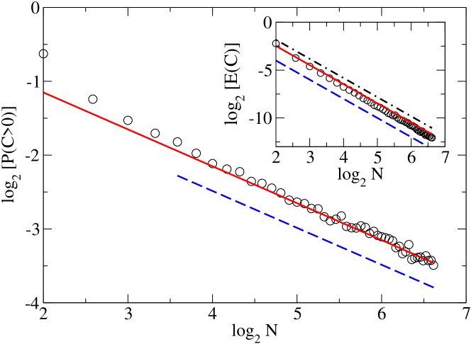
Figure 1: The scaling of $\mbox{Pr}(C>0)$ for random two particle states with $N$ qubits. The dashed line is of slope $-1/2$, the circles are from numerical simulations, while the solid line is the estimate in Eq. (15). Inset shows the average concurrence, the dashed line is of slope $-2$, the dashed-dot line is the upper-bound while the solid line is the estimate in Eq. (17).

For $l=3$, three particle states, a completely different behavior is obtained as $\mu_{1}\sim N^{2}/2$, $\mu_{2}\sim N$, and $\gamma\sim N^{3}/3$ which result in

$$\mbox{Pr}(C>0)<\sqrt{\frac{2}{\pi\,N}}\exp\left(-\frac{N}{2}\log(N/3)\right).$$ (16)

Unlike the two-particle case the probability that the concurrence is positive decreases at least exponentially with the number of qubits, see Fig. (2). Another new feature is that it is quite essential to take into account the fluctuations in both $|a_{12}|$ and in $a_{33}$. Ignoring say the fluctuations in $a_{33}$ results in much smaller estimates of the probability than what is found.

When $l>2$, but still much less than $N$, the upper-bound in Eq. (14) does not estimate the probability accurately. While it can be made tighter, this is indeed a good bound as it is simple, decreases with $N$, and shows the advertized transition in the entanglement as one particle is added to a two particle state. It will be seen that the entanglement hitherto shared between two qubits will now be available for three-body and multi-party entanglement.

If the fraction of particles $p=l/N$ is of order 1 (and less than $1/2$), the states are “macroscopically” occupied; employing the approximation that ${N\choose Np}\sim e^{SN}$ where $S=-p\ln(p)-(1-p)\ln(1-p)$ is the binary entropy corresponding to probability $p$, results in the upper bound $\mbox{Pr}(C>0)<d_{1}e^{-SN/2}\,e^{-d_{2}e^{SN}}$, where $d_{1}$ and $d_{2}$ are positive constants of order 1. However the upper-bound in Eq. (14) has to be used with caution as it can be rendered trivial if $(2\mu_{1}\eta/\gamma)>1$, and consequently $d_{2}$ becomes negative. Thus for $N=10$ qubits and $l=5$ particles the upper-bound $\approx 2.2$ is trivial while for $l=4$ it is $\approx 1.5\times 10^{-5}$. While $N=12$, $l=6$ results in a trivial bound, $l=5$ results in $\mbox{Pr}(C>0)<3.3\times 10^{-15}$. Similarly when $N=14$ and $l=6$, the upper-bound is $\approx 1.6\times 10^{-43}$, it is improbable that two qubits will be entangled.

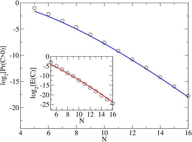
Figure 2: The probability $\mbox{Pr}(C>0)$ for three particle states, and the average concurrence as number of qubits $N$ is changed. Note that the y-axes are on a logarithmic scale. The circles are from numerical simulations while the solid line in the case of $\mbox{Pr}(C>0)$ is from an exact numerical evaluation of Eq. (12).

The mean concurrence, $\mathbb{E}(C)$ is now estimated. In the two particle case for instance

$$\mathbb{E}(C)\sim 2\langle|a_{12}|\rangle\mbox{Pr}(C>0)\sim\dfrac{16}{\pi^{3/2}N^{2}}.$$ (17)

A more general estimate is possible as $\mathbb{E}(C)=\mathbb{E}[2(x-\sqrt{\langle a_{00}\rangle}y)\Theta(x-\sqrt{\langle a_{00}\rangle}y)]$. Using the distribution $P_{12}(x)P_{33}(y)$ and following the same steps as outlined for the probability above it follows that

$$\mathbb{E}(C)<\dfrac{2^{\mu_{2}+2}}{\mathcal{N}\gamma^{\mu_{2}/2}\sqrt{\pi}}\dfrac{\Gamma\left(\frac{\mu_{1}+\mu_{2}+1}{2}\right)}{\Gamma\left(\frac{\mu_{1}}{2}\right)}<\frac{2\sqrt{\gamma}}{\mathcal{N}\sqrt{\pi}}\left(\dfrac{2\mu_{1}\eta^{\prime}}{\gamma}\right)^{\frac{\mu_{2}+1}{2}}$$ (18)

where $\eta^{\prime}=1+(\mu_{2}-1)/(2\mu_{1})$. In the two particle case this gives $\mathbb{E}(C)<8/\sqrt{\pi}N^{2}$, which is quite close to the estimate above. The exponential decay for three or more particles is manifest. The mean concurrences are shown in the insets of Figs. (1),(2).

III.2 Log-negativity among two qubits

The vanishingly small two qubit entanglement for more than two-particle states ($l=2$) goes into multiparty entanglement. A measure of entanglement that can be easily extended to a subsystem having more than two qubits is the log-negativity Vidal and Werner (2002) and is given by $E_{LN}(\rho^{AB})=\log(||\rho_{AB}^{\Gamma}||),$ where $||\rho^{\Gamma}||$ is the trace norm of the partial transpose matrix $\rho^{\Gamma}$ Peres (1996). When log-negativity is zero the state is said to have positive partial transpose (PPT) and in that case it is either separable or bound entangled Horodecki et al. (1998). When log-negativity is greater than zero the state is said to have negative partial transpose (NPT) and in that case it is entangled.

On studying entanglement in a block length of $2$ we get the entanglement between two qubits as measured by log-negativity. This decays algebraically as $1/N^{3.5}$ in contrast to the $1/N^{2}$ behavior of the concurrence for the case of two particles, but becomes exponential when the particle number is increased to three or more. See Fig. (3) for details. Thus on using a different measure of entanglement while indeed the exponents change the qualitative nature of the decay with the number of particles remains intact. It is also useful to contrast the case of 1-particle states and therefore log-negativity is now derived between any two qubits for both 1- and 2-particle states.

III.2.1 Block of 2 qubits and 1-particle states

In this case the reduced density matrix is block diagonal consisting of two square block and is given as follows:

$$\rho_{A}=\left(\begin{matrix}a_{00}&0&0&0\\ 0&a_{11}&a_{12}&0\\ 0&a_{12}^{*}&a_{22}&0\\ 0&0&0&0\\ \end{matrix}\right),$$ (19)

where, $a_{00}=\sum_{i=1}^{N-2}(c_{1i}^{(0)})^{2}$, and

$$\left(\begin{matrix}a_{11}&a_{12}\\ a_{12}^{*}&a_{22}\\ \end{matrix}\right)=Q_{1}Q_{1}^{\dagger},\mbox{and}\;Q_{1}=\left(\begin{matrix}c_{11}^{(1)}\\ c_{21}^{(1)}\\ \end{matrix}\right),$$ (20)

where to remind the reader the coefficients $c_{ij}$ are as defined in Eq. (1).

Partial transpose (PT) on the second qubit of $\rho_{A}$ results in

$$\rho_{A}^{\Gamma}=\left(\begin{matrix}a_{00}&0&0&a_{12}\\ 0&a_{11}&0&0\\ 0&0&a_{22}&0\\ a_{12}^{*}&0&0&0\\ \end{matrix}\right).$$ (21)

The eigenvalues of $\rho_{A}^{\Gamma}$ (as always in this paper, for the case of real coefficients ${c_{ij}^{(k)}}$) are $\Lambda_{\pm}=(a_{00}\pm\sqrt{(a_{00})^{2}+4a_{12}^{2}})/2$, $a_{11}$ and $a_{22}$. The only negative eigenvalue is $\Lambda_{-}$. From the assumptions of randomness of the state, for one-particle states we see that $a_{00}\sim 1$, $a_{12}^{2}\sim 1/N^{2}$. Using this the negative eigenvalue can be approximated by $-a_{12}^{2}/a_{00}\;\sim\;-a_{12}^{2}$. The log-negativity is given by $E_{LN}=\log(1-2\sum_{i}\omega_{i})\approx-2\sum_{i}\omega_{i}\approx 2a_{12}^{2}\approx 2/N^{2}$, where the sum is over all the negative eigenvalues ($\omega_{i}$) of $\rho_{A}^{\Gamma}$ and the approximation holds good since the $\omega_{i}$’s are much smaller than $1$. Indeed one finds that this estimate is in good agreement with the numerical results shown in Fig. (3). Note that the average concurrence between any two qubits for 1-particle states scales as $1/N$ Lakshminarayan and Subrahmanyam (2003).

III.2.2 Block of 2 qubits and 2-particle states

In this case reduced density matrix is block diagonal consisting of three square block and is given as in Eq. (6). Partial transpose on the second qubit of $\rho_{A}$ results in

$$\rho_{A}^{\Gamma}=\left(\begin{matrix}a_{00}&0&0&a_{12}\\ 0&a_{11}&0&0\\ 0&0&a_{22}&0\\ a_{12}^{*}&0&0&a_{33}\\ \end{matrix}\right).$$ (22)

The eigenvalues of this are

$$\Lambda_{\pm}=\dfrac{1}{2}\left(a_{00}+a_{33}\pm\sqrt{(a_{00}+a_{33})^{2}-4(a_{00}a_{33}-a_{12}^{2})}\right)$$

and the pair of $a_{11}$ and $a_{22}$. Again the only possible negative eigenvalue is $\Lambda_{-}$ which occurs when $a_{00}a_{33}-a_{12}^{2}$ is negative. In the case of two-particle sates, as we see earlier, $a_{00}\sim 1$, $a_{12}^{2}\sim 4/N^{3}$ and $a_{33}\sim 1/N^{2}$ and thus the eigenvalue $\Lambda_{-}$ can be approximated by $(a_{00}a_{33}-a_{12}^{2})/(a_{00}+a_{33})\;\sim\;a_{00}a_{33}-a_{12}^{2}$. Thus $E_{LN}=2a_{12}^{2}\;$Pr$((a_{00}a_{33}-a_{12}^{2})<0)$. Using Eq. (15) we find that

$$E_{LN}\sim\dfrac{16\sqrt{2}}{\pi}\dfrac{1}{N^{3.5}}$$

which is in good agreement with the numerical results shown in Fig. (3). In the case of a block of 2 qubits and 3-particle states one finds that the log-negativity scales exponentially with the total number of qubits $N$ as shown in Fig. (3). This follows on using the exponentially small probability for the concurrence to be positive (see Eq.  (16)) and a similar analysis as above.

IV Entanglement among larger subsets of qubits

While the previous section has dealt exclusively with a “block” of two qubits, here we take larger subsets of qubits to belong to block $A$. The Log-negativity measure will be used once again. A transition similar to the one above is exhibited for the entanglement between a qubit and the other pair when a block of $3$ qubits is considered. Algebraic decay of the log-negativity for $l\leq 3$ is replaced by exponential decay for $l>3$, see Fig. (4). The decay with particle number is algebraic and the exponent is the “slope” in Table 1. Further results for block lengths of 4 are presented in Table 2, in which case there are two distinct types of partitions, entanglement between two pairs of qubits (denoted as 2+2) and between a triple and a lone qubit (denoted 3+1). However the numerics becomes considerably more difficult thereon, and the slopes given may not be entirely converged. However, the transition from algebraic to exponential is a robust feature.

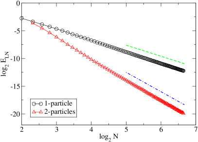
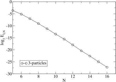
Figure 3: Scaling of log-negativity ($E_{LN}$) in a block of 2 qubits, with the total number $N$ of qubits for (left) one, two-particle and (right) three-particle states. In figure on left dashed line, dashed-dot line are having slope of -2, -3.5 respectively.

Table 1: Block length 3.

Particle # ($l$)	Decay with number of qubits $N$.
1	Alg.: slope = -2
2	Alg.: slope = -3
3	Alg.: slope = -4.5
4	Exponential

Table 2: Block length 4. Cases of (2+2,3+1)

Particle # ($l$)	Decay with number of qubits $N$.
1	Alg.: slopes = (-2.1, -2.1)
2	Alg.: slopes = (-2.1, -3.1)
3	Alg.: slopes = (-4.1, -4.1)
4	Alg.: slopes = (-5.7, -5.7)
5	Exponential

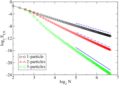
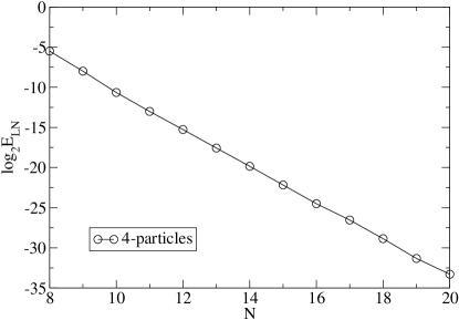
Figure 4: Scaling of log-negativity ($E_{LN}$) in a block of 3 qubits, with the total number $N$ of qubits for (left) one, two and three-particle and (right) four-particle states. In figure on left dashed line, dashed-dot line and simple straight line are having slope of -2, -3, -4.5 respectively.

It is possible to extend the analysis of the log-negativity of two qubits to the case of a block of three qubits and derive some of the exponents as stated in the table. Now large $N$ formulae for log-negativity in the case of a block of 3 qubits in 1-particle and 2-particle states are derived. It is shown that the log-negativity decays as $4/N^{2}$, $16/N^{3}$ for these cases respectively.

IV.0.1 Block of 3 qubits and 1-particle case.

In this case the reduced density matrix is block diagonal consisting of two square blocks, one of them ($a_{00}$) being just a number:

$$\rho_{A}=\left(\begin{matrix}a_{00}&0_{1\times 3}&0_{1\times 4}\\ 0_{3\times 1}&Q_{1}Q_{1}^{\dagger}&0_{3\times 3}\\ 0_{4\times 1}&0_{4\times 3}&0_{4\times 4}\\ \end{matrix}\right),$$ (23)

where $a_{00}=\sum_{i=1}^{N-3}(c_{1i}^{(0)})^{2}$, $0_{p\times q}$ are zero matrices with dimensions $p\times q$ and

$$Q_{1}Q_{1}^{\dagger}=\left(\begin{matrix}a_{11}&a_{12}&a_{13}\\ a_{12}^{*}&a_{22}&a_{23}\\ a_{13}^{*}&a_{23}^{*}&a_{33}\\ \end{matrix}\right),\;Q_{1}=\left(\begin{matrix}c_{11}^{(1)}\\ c_{21}^{(1)}\\ c_{31}^{(1)}\\ \end{matrix}\right).$$ (24)

Being 1-particle states these have only two nonzero eigenvalues in general. On PT it is seen that there are four nonzero eigenvalues. Partial transpose on the third qubit of $\rho_{A}$ results in

$$\rho_{A}^{\Gamma}=\left(\begin{matrix}a_{00}&0&0&0&a_{12}&a_{13}&0&0\\ 0&a_{11}&0&0&0&0&0&0\\ 0&0&a_{22}&a_{23}&0&0&0&0\\ 0&0&a_{23}^{*}&a_{33}&0&0&0&0\\ a_{12}^{*}&0&0&0&0&0&0&0\\ a_{13}^{*}&0&0&0&0&0&0&0\\ 0&0&0&0&0&0&0&0\\ 0&0&0&0&0&0&0&0\\ \end{matrix}\right).$$ (25)

The nonzero eigenvalues of $\rho^{\Gamma}$ are $a_{11}$, $a_{22}+a_{33}$ and

$$\Lambda_{\pm}=\dfrac{1}{2}\left(a_{00}\pm\sqrt{a_{00}^{2}+4(a_{12}^{2}+a_{13}^{2})}\right).$$

Note that there are correlations in the entries of the $Q_{1}Q_{1}^{\dagger}$ matrices, such as $a_{22}a_{33}-a_{23}^{2}=0$ as the state from the density matrix is constructed is an (unnormalized) pure state. Here $a_{00}\sim 1$, $a_{12}^{2}$ and $a_{13}^{2}\sim 1/N^{2}$. It can be seen that only one of the four nonzero eigenvalues is negative and it is $\Lambda_{-}$. Using this, the negative eigenvalue can be approximated as $-(a_{12}^{2}+a_{13}^{2})/a_{00}\approx-(a_{12}^{2}+a_{13}^{2})$. The log-negativity is therefore given by $E_{LN}\approx-2\sum_{i}\omega_{i}\approx 2(a_{12}^{2}+a_{13}^{2})\approx 4/N^{2}$. This estimate is in good agreement with numerical results as shown in Fig. (4).

IV.0.2 Block of 3 qubits and 2-particle case.

In this case the reduced density matrix is block diagonal consisting of three square blocks and is given as follows:

$$\rho_{A}=\left(\begin{matrix}a_{00}&0_{1\times 3}&0_{1\times 3}&0_{1\times 1}\\ 0_{3\times 1}&Q_{1}Q_{1}^{\dagger}&0_{3\times 3}&0_{3\times 1}\\ 0_{3\times 1}&0_{3\times 3}&Q_{2}Q_{2}^{\dagger}&0_{3\times 1}\\ 0_{1\times 1}&0_{1\times 3}&0_{1\times 3}&0_{1\times 1}\\ \end{matrix}\right),$$ (26)

where $a_{00}=\sum_{i=1}^{\alpha_{0}}(c_{1i}^{(0)})^{2}$, and

$$Q_{1}Q_{1}^{\dagger}=\left(\begin{matrix}a_{11}&a_{12}&a_{13}\\ a_{12}^{*}&a_{22}&a_{23}\\ a_{13}^{*}&a_{23}^{*}&a_{33}\\ \end{matrix}\right),\;Q_{1}=\left(\begin{matrix}c_{11}^{(1)}&\ldots&c_{1\alpha_{1}}^{(1)}\\ c_{21}^{(1)}&\ldots&c_{2\alpha_{1}^{(1)}}\\ c_{31}^{(1)}&\ldots&c_{3\alpha_{1}^{(1)}}\\ \end{matrix}\right),$$ (27)

$$Q_{2}Q_{2}^{\dagger}=\left(\begin{matrix}a_{44}&a_{45}&a_{46}\\ a_{45}^{*}&a_{55}&a_{56}\\ a_{46}^{*}&a_{56}^{*}&a_{66}\\ \end{matrix}\right),\;Q_{2}=\left(\begin{matrix}c_{11}^{(2)}\\ c_{21}^{(2)}\\ c_{31}^{(2)}\\ \end{matrix}\right).$$ (28)

Here $\alpha_{i}={N-3\choose 2-i},\;i=0,1,2$. Partial transpose on the third qubit of $\rho_{A}$ results in

$$\rho_{A}^{\Gamma}=\left(\begin{matrix}a_{00}&0&0&0&a_{12}&a_{13}&0&0\\ 0&a_{11}&0&0&0&0&0&0\\ 0&0&a_{22}&a_{23}&0&0&0&a_{46}\\ 0&0&a_{23}^{*}&a_{33}&0&0&0&a_{56}\\ a_{12}^{*}&0&0&0&a_{44}&a_{45}&0&0\\ a_{13}^{*}&0&0&0&a_{45}^{*}&a_{55}&0&0\\ 0&0&0&0&0&0&a_{66}&0\\ 0&0&a_{46}^{*}&a_{46}^{*}&0&0&0&0\\ \end{matrix}\right).$$ (29)

In this case, while the density matrix has one zero eigenvalue, the partial transpose has no zero eigenvalue. Apart from the eigenvalues $a_{11}$ and $a_{66}$, the other six eigenvalues are those of the matrices $A$ and $B$, where:

$$A=\left(\begin{matrix}a_{00}&a_{12}&a_{13}\\ a_{12}^{*}&a_{44}&a_{45}\\ a_{13}^{*}&a_{45}^{*}&a_{55}\\ \end{matrix}\right),\;B=\left(\begin{matrix}a_{22}&a_{23}&a_{46}\\ a_{23}^{*}&a_{33}&a_{56}\\ a_{46}^{*}&a_{56}^{*}&0\\ \end{matrix}\right).$$ (30)

The characteristic equation of matrix $A$ is

$$\lambda^{3}-\lambda^{2}(a_{00}+a_{44}+a_{55})-\lambda(a_{45}^{2}+a_{12}^{2}+a_{13}^{2}-a_{00}a_{44}-a_{00}a_{55}-a_{44}a_{55})$$ (31)

$$+(a_{00}a_{45}^{2}+a_{55}a_{12}^{2}+a_{44}a_{13}^{2}-a_{55}a_{00}a_{44}-2a_{12}a_{13}a_{45}) = 0.$$

Here we see that average of coefficients of $\lambda^{2}$ and $\lambda$ goes as $-1-2/N^{2}$ and $4/N^{2}$ while that of constant term goes as $16/N^{5}$. Thus typically the determinants of $A$ and $B$, which are the negative of the constant term, are negative, and hence the three eigenvalues of each matrix can either all be negative or have one lone negative value. That the latter is the case follows on noting that the traces of these two matrices are positive.

One may estimate the negative eigenvalue now. Assuming that the terms containing $\lambda^{3}$ and $\lambda^{2}$ are of smaller order, and keeping only the linear and constant terms one gets that the negative eigenvalues of $A$ is approximately $-4/N^{3}$. It is immediately verified that the assumptions just made are justified. The characteristic equation of matrix $B$ is

$$\lambda^{3}-\lambda^{2}(a_{22}+a_{33})-\lambda(a_{56}^{2}+a_{46}^{2}+a_{23}^{2}-a_{22}a_{33})+a_{22}a_{56}^{2}+a_{33}a_{46}^{2}-2a_{23}a_{46}a_{56}=0.$$

The average of the coefficients of $\lambda^{2}$ and $\lambda$ go as $-2/N$ and $4/N^{2}$ while that of the constant term goes as $16/N^{5}$. Using an argument similar to that used to approximate the negative eigenvalue of the matrix $A$, we can approximate the same for matrix $B$ as $-4/N^{3}$. The log-negativity is given by $E_{LN}\approx-2\sum_{i}\omega_{i}\approx 8/N^{3}+8/N^{3}=16/N^{3}$. This estimate is again in very good agreement with numerical results as shown in Fig. (4), including both the exponent and the constant.

V Density of states before and after PT

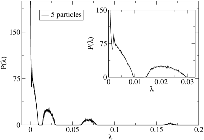
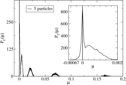
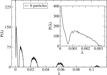
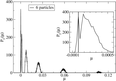
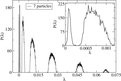
Figure 5: Density of states of the reduced density matrix $\rho_{A}$ (left column) and its partial transpose $\rho_{A}^{\Gamma}$ (right column). The block length ($m$) is equal to $6$, the total number of qubits ($N$) is $22$ and the particle number ($l$) varies as shown. The insets shows an enlarged view of the region near the origin of the respective figures. In the insets of the right column a vertical line at the origin has been shown to draw attention to the negative part of the spectrum.

The spectral properties of the reduced density matrix which represents the state of the block whose entanglement is under investigation is of natural interest. Apart from being positive semi-definite the eigenvalues of the reduced density matrix of a pure random state has a characteristic distribution or “density of states”, which is discussed further below. In contrast the corresponding spectrum for the partial transpose need not be positive semi-definite; indeed if the density of states now of the PT of the reduced density matrix, has support in the negative numbers, the corresponding state is entangled or NPT. The mechanism that is responsible for the transitions pointed to above remains to be fully investigated, however the density of states of the reduced density matrix may be playing a crucial role.

To elucidate this, as discussed in the Introduction, when $l<m$, that is the number of particles is smaller than the block length, there are many exact zero eigenvalues in the density matrix $\rho_{A}$, in contrast when $l\geq m$ the density matrix becomes of full rank. In fact when $l=m$ a detailed study of the density matrix shows a density of states that still diverges at 0, while for $l>m$ the density of states vanishes at zero. Negative eigenvalues develop in the partial transpose of the rank-deficient matrices corresponding to the case $l<m$. When the density of states of $\rho_{A}$ is bounded away from zero, as in the case of $l>m$, the partial transpose is also bounded away from zero and has typically only positive eigenvalues. In the marginal case when $l=m$ the divergent density of states of $\rho_{A}$ seems to lead to negative partial transpose. Thus whenever a density matrix has exact zero eigenvalues, or has a divergent density of states at zero, it will be typically NPT, and hence entangled. As the number of particles is increased beyond the block size, the spectrum of $\rho_{A}$ gets bounded away from zero and it becomes PPT. Thus the transition seems to originate in the transition of the density of states of the reduced density matrix, which in turn is due to the rank of the density matrix becoming full at the point of transition. However we emphasize that the observations made here are partially numerical and further work on the partial transpose of rank-deficient matrices is necessary to justify them rigorously.

If $|\psi\rangle$ is a full random state of $N$ qubits, mixing all particle numbers together, and let the subset $A$ have Hilbert space dimension $d_{A}$ and the complementary set, dimension $d_{B}$ ($d_{A}\leq d_{B}$). Then the density of states of the reduced density matrix of a subset $A$ of the qubits $\rho_{A}$, if $d_{A},d_{B}\gg 1$, will typically be distributed according to the Marcenko-Pastur rule Marcenko and Pastur (1967):

$$\begin{split}f(\lambda)&=\frac{d_{A}Q}{2\pi}\frac{\sqrt{(\lambda_{max}-\lambda)(\lambda-\lambda_{min})}}{\lambda}\\ {\lambda_{min}^{max}}&=\frac{1}{d_{A}}\bigg{(}1+\frac{1}{Q}\pm\frac{2}{\sqrt{Q}}\bigg{)};\;\;Q=d_{B}/d_{A}.\end{split}$$ (32)

In the “symmetric” case of $Q=1$, the density of states diverges at the origin, else it is bounded away from zero. In fact much is known about the distribution of the smallest eigenvalue in the symmetric case, including its distribution and average ($1/d_{A}^{3}$) Majumdar et al. (2008).

Corresponding questions for definite particle subspaces are of natural interest, and we present some results here for the density of states, but only in so far as they pertain to the problem of entanglement transition studied above. Thus in addition to the density of states, $P(\lambda)$ of the density matrix $\rho_{A}$ the density of states, $P_{\Gamma}(\mu)$, of the partial transpose, $\rho_{A}^{\Gamma}$ is of interest. In Fig. (5) is shown the density of states before and after the partial transposition for a case when there are $N=22$ qubits in all. The block $A$ consists of $m=6$ qubits and the density of states is shown as the particle number is changed across this value. Looking at the density of states $P(\lambda)$ for the case $l=6$ particles one can see the divergence at the origin as well as several clumps of eigenvalues. The origin of the clumps is quite easily understood as arising from the individual $G_{k}$ blocks acting as practically independent density matrices, the trace normalization condition being the only constraint amongst them. These individual blocks then tend to have density of states that are of the nature of the Marcenko-Pastur distribution with suitable dimensions. Thus roughly, especially for large $N$, the density of states is pretty much a superposition of such distributions.

The eigenvalues $\lambda$ of the extreme nonzero blocks $G_{0}$ and $G_{r}$ where $r=m$ or $l$ depending on whether $l\geq m$ or $<m$, are special in the sense that there is only a lone nonzero eigenvalue and they do not follow the Marcenko-Pastur distribution. In any case the “block” $G_{0}$ is just a number, while $G_{r}$ is a matrix for $l<m$ and a number for $l\geq m$. For example in the case when $m=2$, these two numbers are the values of $a_{00}$ and $a_{33}$ of Eq. (6), which are seen to be the sum of squares of the normally distributed coefficients. Therefore it is easy to see that in general they are chi-squared distributed with number of degrees of freedom $d$:

$$\frac{1}{2^{d/2}\Gamma(d/2)}\;x^{d/2-1}e^{-x/2},\;\;x\in[0,\infty)\;\mbox{and}\;d\geq 1,$$ (33)

where $x=\lambda\mathcal{N}$. The number of degrees of freedom $d$ depends on whether $l\leq m$ or $l>m$. In either case for the eigenvalue of $G_{0}$, $d$ is equal to ${N-m\choose l}$. In the case of the eigenvalue of the block $G_{r}$, $d={N-m\choose l-m}$ when $l\geq m$, and $d={m\choose l}$ for $l<m$. Thus when $l=m$, the number of particles is the block size, $d=1$ for the eigenvalue of the block $G_{r}$. Note that when $d=1$ the chi-squared distribution diverges at the origin, unlike the case $d>1$. Thus although at the transition point $l=m$, the density matrix $\rho_{A}$ is of full rank, it has a divergent density of states arising from this eigenvalue. Note that when $l>m$ these lone eigenvalues can never lead to a divergent density of states. Also from the inequality in Eq. (5) it follows that there will never be a symmetric case of the Marcenko-Pastur distribution when $l>m$. Thus indeed this completes the proof that the density of states does not diverge at zero when $l>m$, while it does for $l\leq m$.

Not much is known of the density of states of the partial transpose even for the case of full random states, except for a recent mathematical study Aubrun (2010) and an ongoing work Bhosale et al. which shows for instance that when a density matrix has a symmetric Marcenko-Pastur distribution ($Q=1$), its partial transpose has a semi-circle distribution. Indeed the density of states of the partial transposed matrix $\rho_{A}^{\Gamma}$ as shown in Fig. (5) is not very different from that of the density matrix itself. The important exceptions are cases where the density of states diverges at the origin (in the case of $l=5$ and $6$) and the density of states of $\rho_{A}^{\Gamma}$ clearly has support in the negative numbers, indicating the NPT nature of $\rho_{A}$. In contrast when there are $7$ particles the PT has almost no negative eigenvalues. A much more detailed study of the tails of these distributions show a very small fraction of negative eigenvalues, indicating that entanglement when present is very rare. This is reflected in the exponentially small probability of entangled states after the transition ($l>m$). Thus the origin of the entanglement transitions seems to lie in the change of character of the density of states of the reduced density matrix around zero.

VI Discussions and conclusion

While we have focused on the study entanglement within a block of qubits, one may also ask if transitions are seen in the entanglement of the block with the rest of the qubits, say measured by the von Neumann entropy. Preliminary work not presented here, as well as from the discussions above we believe that no such transition is seen. This is due to the fact that von Neumann entropy is fairly insensitive to the nature of the density of states around the zero eigenvalue. For instance even in the case of full random states, the symmetric states (equal bipartitions) do not possess qualitatively different entanglement entropy from the non-symmetric ones Page (1993). On the other hand, entanglement within the block, as measured by the log-negativity (or the concurrence in the case of two qubits) is sensitive to the presence of a large number of zero or near zero eigenvalues.

In summary this paper has given definitive evidence of a transition in entanglement between two qubits as the number of particles is increased to three. Using log-negativity it is shown that the following generalization would hold: the entanglement content in $m$ qubits decays algebraically with $N$, the number of qubits, if the number of particles $l\leq m$, and exponentially if $l>m$. Various exponents in the case of algebraic decay have been analytically derived for the case of concurrence as well as the log-negativity. The observation of a transition is further strengthened by studying the density of states of the reduced density matrix and its partial transpose. It is shown that the rank of the density matrix is not full till the number of particles is precisely equal to the block size; and that even at exactly the marginal case, the density of states of the reduced density matrix diverges at zero, although it is of full rank. The exact zero eigenvalues or the large number of very small ones seem to translate on partial transpose to negative eigenvalues, thus leading to typically entangled states. This is the case as long as the number of particles is less than or equal to the block size. Otherwise the density of states vanishes at zero and leads to a predominantly positive partial transpose, which results in the exponentially small entanglement.

The question of whether the transition studied is also observed on using other entanglement measures is a natural and interesting one. It is quite easy to see that the negativity measure (rather than the log-negativity studied here) also undergoes such a transition. Note that unlike the log-negativity measure which is not convex but is nevertheless an entanglement monotone Plenio (2005), the negativity measure is both convex and an entanglement monotone Vidal and Werner (2002). While many other measures, such as distillable entanglement Nielsen and Chuang (2000), are difficult to compute, it seems very plausible that the transition is indeed independent of the particular measure used. This is strengthened by the study of the spectra of the reduced density matrix and its partial transpose, and the fact that the transition may well have its origins in the behavior of their density of states.