Yang-Yang method for the thermodynamics of one-dimensional multi-component interacting fermions

Abstract

Using Yang and Yang’s particle-hole description, we present a thorough derivation of the thermodynamic Bethe ansatz equations for a general $SU(\kappa)$ fermionic system in one-dimension for both the repulsive and attractive regimes under the presence of an external magnetic field. These equations are derived from Sutherland’s Bethe ansatz equations by using the spin-string hypothesis. The Bethe ansatz root patterns for the attractive case are discussed in detail. The relationship between the various phases of the magnetic phase diagrams and the external magnetic fields is given for the attractive case. We also give a quantitative description of the ground state energies for both strongly repulsive and strongly attractive regimes.

I Introduction

Exactly solvable models of interacting fermions in one-dimension (1D) have attracted theoretical interest for more than half a century. Before 1950, it was not clear how to treat the Schrödinger equation for a large system of interacting fermions. The first important breakthrough was achieved by Tomonaga Tomonaga1950 who showed that fermionic interactions in 1D can mediate new collective degrees of freedom that are approximately bosonic in nature.

In 1963, Luttinger Luttinger1963 introduced an exactly solvable many-fermion model in 1D which consists of two types of particles, one with positive momentum and the other with negative momentum. However, Luttinger’s model suffers from several flaws which include the assumption that the fermions are spinless and massless, and more importantly an improperly filled negative energy Dirac sea. Mattis and Lieb Mattis1965 expanded on Luttinger’s work by correctly filling the negative energy states with “holes”. Before that, Lieb and Liniger Lieb1963a ; Lieb1963b solved the 1D interacting Bose gas with $\delta$-function interactions using Bethe’s hypothesis Bethe1931 . Later McGuire solved the equivalent spin-1/2 fermion problem for the special case where all fermions have the same spin except one having the opposite spin in the repulsive McGuire1965 and attractive McGuire1966 regimes. He showed that in the presence of an attractive potential a bound state is formed. Further progress by Lieb and Flicker LF followed on the two down spin problem. In 1967, Yang Yang1967 solved the fermion problem for the most general case where the number of spin ups and spin downs are arbitrary by making use of Bethe’s hypothesis. At the same time, Gaudin Gaudin1967 solved this problem for the ground state with no polarization.

Sutherland Sutherland1968 then showed that the fermion model with a general $SU(\kappa)$ spin symmetry is integrable and the solution is given in terms of $\kappa$ nested Bethe ansatz (BA) equations. And in 1970, Takahashi Takahashi1970 examined the structure of the bound states in the attractive regime with arbitrary spin and derived the ground state energy together with the distribution functions of bound states in terms of a set of coupled integral equations. Using Yang and Yang’s method YangYang1969 for the boson case, Takahashi Takahashi1971 and Lai Lai1971 ; Lai1973 derived the so-called thermodynamic Bethe ansatz (TBA) equations for spin-1/2 fermions in both the repulsive and attractive regimes. The spin-string hypothesis describing the excited states of spin rapidities was also introduced by both authors. Later on, Schlottmann Schlottmann1993 ; Schlottmann1994 derived the TBA equations for $SU(\kappa)$ fermions with repulsive and attractive interactions. See also Schlottmann’s epic review article on exact results for highly correlated electron systems in 1D S-review .

The TBA equations have been analyzed in several limiting cases, i.e., $T\rightarrow 0$, $T\rightarrow\infty$, $c\rightarrow 0$ and $|c|\rightarrow\infty$, where $T$ is the temperature and $c$ is the interaction strength. The ground state properties and the elemental charge and spin excitations were also studied for some special cases. However, the TBA equations for the attractive regime Schlottmann1994 ; S-review are not the most convenient for the analysis of phase transitions and thermodynamics. For the attractive case, it was shown that the ground state in the absence of symmetry breaking fields consists of spin neutral charge bound states of $\kappa$ particles. The repulsive case however consists of freely propagating charge states and spin waves with different velocities. The phenomenon of spin-charge separation plays a ubiquitous role in the low energy physics of 1D systems Giamarchi . However, the physics of these models, such as the universal thermodynamics of Tomonaga-Luttinger liquids, quantum criticality and the universal nature of contact interaction, are largely still hidden in the complexity of the TBA equations. It is thus important to develop new methods to extract the physics of 1D exactly solved many-body systems in order to bring them more closer to experiments.

Most recently, experimental advances in trapping and cooling atoms to very low temperatures allow a test of the theoretical predictions made so far. In particular, Liao et al. Liao2009 experimentally studied spin-1/2 fermions of ultracold ⁶Li atoms in a 2D array of 1D tubes with spin imbalance. The phase diagram was confirmed and it was discovered that a large fraction of a Fulde-Ferrell-Larkin-Ovchinnikov (FFLO)-like phase lies in the trapping center accompanied by two wings of a fully paired phase or unpaired phase depending on the polarization. This observation verified the theoretical predictions Orso ; Hu ; Guan2007 ; Mueller regarding the phase diagram and pairing signature for the ground state of strongly attractive spin-1/2 fermions in 1D. Although the FFLO phase has not yet been observed directly, the experimental results pave the way to direct observation and characterization of FFLO pairing Liao2009 .

In this paper, we derive the TBA equations for a general 1D system of fermions with $SU(\kappa)$ spin symmetry from Sutherland’s BA equations using the same approach as Yang and Yang for 1D bosons YangYang1969 . Both the repulsive and attractive cases are discussed. We also give the exact thermodynamics of the ground state of the attractive and repulsive cases in both the strong coupling and weak coupling limits. A general relationship between the different magnetic phases and the external magnetic field is discussed for the attractive case. How the external magnetic fields affect the different pairing phases in the attractive regime is also addressed. This paper gives a thorough derivation of many results in a recently published paper Guan2010 that provides the exact low temperature thermodynamics for strongly attractive $SU(\kappa)$ fermions with Zeeman splitting and shows that the system behaves like a universal Tomonaga-Luttinger liquid in the gapless phase.

II The Model

The Hamiltonian for the 1D $N$-body problem is

$$H=-\frac{\hbar^{2}}{2m}\sum_{i=1}^{N}\frac{\partial^{2}}{\partial x_{i}^{2}}+g_{1D}\sum_{1\leq i<j\leq N}\delta(x_{i}-x_{j})+\sum_{i=1}^{\kappa}N^{i}\epsilon^{i}_{Z}(\mu_{B}^{i},B).$$ (1)

It describes $N$ fermions of the same mass $m$ confined to a 1D system of length $L$ interacting via a $\delta$-function potential. The first and second terms in the Hamiltonian correspond to the kinetic energy and $\delta$-interaction potential respectively. The coupling constant $g_{1D}$ can be expressed in terms of the interaction strength $c=2/a_{1D}$ as $g_{1D}=-\hbar^{2}c/m$ where $a_{1D}$ is the effective 1D scattering length. For repulsive fermions, $c>0$ and for attractive fermions, $c<0$. We shall assume that the system has periodic boundary conditions i.e., $\psi(x_{1},\ldots,x_{i},\ldots,x_{N})=\psi(x_{1},\ldots,x_{i}+L,\ldots,x_{N})$ where $x_{i}$ is the position of the $i$-th particle. There will be $\kappa$ possible hyperfine states $|1\rangle,|2\rangle,\ldots,|\kappa\rangle$ that the fermions can occupy. The number of fermions in the state $|i\rangle$ is given by $N^{i}$ while the Zeeman energy $\epsilon^{i}_{Z}$ is determined by the magnetic moment $\mu^{i}_{B}$ and the magnetic field $B$. For brevity, we shall choose the dimensionless units $\hbar=2m=1$ for the rest of this paper.

The wavefunction $\psi$ for this Hamiltonian satisfies the symmetry of an irreducible representation $R_{\psi}=[\kappa^{N^{\kappa}},(\kappa-1)^{N^{\kappa-1}-N^{\kappa}},\ldots,2^{N^{2}-N^{3}},1^{N^{1}-N^{2}}]$, where the $N^{i}$s are such that $N^{1}\geq N^{2}\geq\ldots\geq N^{\kappa}$. The Young tableau which corresponds to this irreducible representation is given in FIG. 1. This system has $SU(\kappa)$ spin symmetry and $U(1)$ charge symmetry. Sutherland Sutherland1968 showed that this problem can be solved by repeatedly using the generalized Bethe’s hypothesis which was introduced by Yang Yang1967 . To obtain the total momentum $p=\sum_{j=1}^{N}k_{j}$ and the energy eigenspectrum $E=\sum_{j=1}^{N}k_{j}^{2}$ for the system, we need to find a set of quasimomenta $k_{j}$ that satisfies the equations

$$\exp(ik_{j}L)=\prod_{l=1}^{M_{1}}\frac{k_{j}-\Lambda^{(1)}_{l}+ic^{\prime}}{k_{j}-\Lambda^{(1)}_{l}-ic^{\prime}}\qquad j=1,\ldots,N$$ (2)

$$\prod_{\beta=1}^{M_{p-1}}\frac{\Lambda_{\alpha}^{(p)}-\Lambda_{\beta}^{(p-1)}+ic^{\prime}}{\Lambda_{\alpha}^{(p)}-\Lambda_{\beta}^{(p-1)}-ic^{\prime}}=-\prod_{\gamma=1}^{M_{p}}\frac{\Lambda_{\alpha}^{(p)}-\Lambda_{\gamma}^{(p)}+2ic^{\prime}}{\Lambda_{\alpha}^{(p)}-\Lambda_{\gamma}^{(p)}-2ic^{\prime}}\prod_{\delta=1}^{M_{p+1}}\frac{\Lambda_{\alpha}^{(p)}-\Lambda_{\delta}^{(p+1)}-ic^{\prime}}{\Lambda_{\alpha}^{(p)}-\Lambda_{\delta}^{(p+1)}+ic^{\prime}}$$

$$\alpha=1,\ldots,M_{p}\qquad\textrm{and}\qquad p=1,\ldots,\kappa-1$$ (3)

where $M_{0}:=N$, $M_{\kappa}=0$, $\Lambda_{j}^{(0)}:=k_{j}$ and $\Lambda_{j}^{(\kappa)}$ is undefined. The rapidities $\Lambda_{j}^{(p)}$ characterize the internal spin degrees of freedom. The quantum numbers $M_{i}$ are defined as $M_{i}=\sum_{j=i}^{\kappa-1}N^{j+1}$ and $c^{\prime}=c/2$. This set of $\kappa$ coupled algebraic equations are called the BA equations.

Figure 1: The Young tableau which corresponds to the irreducible representation $R_{\psi}=[\kappa^{N^{\kappa}},(\kappa-1)^{N^{\kappa-1}-N^{\kappa}},\ldots,2^{N^{2}-N^{3}},1^{N^{1}-N^{2}}]$.

III The root pattern

We shall only consider the strong coupling regime where $L|c|\gg 1$. For the repulsive case, it is easily shown that the roots $k_{j}$ must be real Takahashi . However the rapidities $\Lambda_{j}^{(p)}$ are allowed to take on nonzero imaginary values. It was first suggested by Lai Lai1971 that the rapidities appear as strings in the complex plane of the form

$$\Lambda_{\alpha}^{(p),n,j}=\Lambda_{\alpha}^{(p),n}+i(n+1-2j)|c^{\prime}|+O(\exp(-\delta L))\qquad j=1,\ldots,n$$ (4)

in the thermodynamic limit where $N,L\rightarrow\infty$ while keeping the ratio $N/L$ fixed. Here $n$ is the length of the string, $\alpha$ labels each individual string and $\Lambda_{\alpha}^{(p),n}$ denotes the real part of each string. Every string must be symmetric along the real axis, i.e. any complex solution is accompanied by its complex conjugate pair. This solution for the rapidities hold as long as $L|c|\gg 1$. In other words, it holds up to order $\exp(-\delta L)$ where $\delta$ is a positive monotonic increasing function of the interaction strength $|c|$. When the system is in its ground state, the rapidities do not form strings. The strings also obey the relation $M_{p}=\sum_{n=1}^{\infty}nM_{n}^{(p)}$ where $M_{n}^{(p)}$ is the number of $\Lambda_{j}^{(p)}$ strings with length $n$.

In the attractive regime, it is found that complex string solutions of $k_{j}$ also satisfy the BA equations. A system with $\kappa$-components of fermions has $SU(\kappa)$ symmetry. The quasimomenta $k_{j}$ may appear as bound states of up to length $\kappa$. For convenience, we denote the number of $k_{j}$ bound states with length $1\leq i\leq\kappa$ as $N_{i}$. In the ground state, none of the bound states can be broken which means that $N_{i}=N^{i}-N^{i+1}$. A bound state in $k$-space of length $m$ will take the form

$$k_{\alpha}^{m,j}=\lambda_{\alpha}^{(m-1)}+i(m+1-2j)|c^{\prime}|+O(\exp(-\delta L))\qquad j=1,\ldots,m$$ (5)

with real part $\lambda_{\alpha}^{(m-1)}$. In general, a $k_{\alpha}$ bound state of length $m$ will be accompanied by a $\Lambda_{\alpha}^{(1)}$ bound state of length $m-1$, a $\Lambda_{\alpha}^{(2)}$ bound state of length $m-2$ and so on until a $\Lambda_{\alpha}^{(m-1)}$ bound state of length $1$. Each accompanying bound state in $\Lambda^{(1)}$-space, $\Lambda^{(2)}$-space, …, $\Lambda^{(m-1)}$-space will share the same real part $\lambda_{\alpha}^{(m-1)}$. A graphical depiction is given in FIG. 2.

However, strings in $\Lambda^{(p)}$-space do not have to be accompanied by any shorter string. Therefore, the difference between our definition of a bound state and a string is that a bound state is a string that originates from $k$-space, and is accompanied by corresponding strings in each subsequent $\Lambda^{(p)}$-space. On the other hand a string in $\Lambda^{(p)}$-space characterizes the spin excitations that can exist independently in spin sectors.

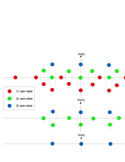
Figure 2: (Color online) Root pattern for the $\kappa=3$ case with $N=23$, $N^{1}=13$, $N^{2}=7$ and $N^{3}=3$ in the ground state ($T=0$). Bounds states are formed for charge and spin rapidities and are indicated by the dashed boundaries. Accompanying bound states in each subsequent $\Lambda^{(p)}$-space share the same real part. The maximum length of any bound state in $k$-space is $\kappa=3$. In an excited state ($T>0$), strings can also form in $\Lambda^{(p)}$-space.

IV The TBA equations: Repulsive case

The TBA equations which are expressed in the form of dressed energies allow us to precisely derive numerous thermodynamic quantities and to analyze the behavior of phase transitions at critical points. Explicit expressions for the free energy, grand partition function, pressure, chemical potential and so on can be directly obtained from the TBA equations. Physically, the TBA equations give us the energy of elementary excitations above the ground state. There are several steps to take in order to derive these equations. We will give an outline of each step in deriving these equations for the repulsive case, all of which follow from Yang and Yang’s pioneering work YangYang1969 .

The string solution for $\Lambda_{j}^{(p)}$ gives us a different form of the BA equations when substituted into the original equations (2) and (3). After lengthy calculations, we obtain

$$\exp(ik_{j}L)=\prod_{n=1}^{\infty}\prod_{\alpha=1}^{M_{n}^{(1)}}\frac{k_{j}-\Lambda_{\alpha}^{(1),n}+inc^{\prime}}{k_{j}-\Lambda_{\alpha}^{(1),n}-inc^{\prime}}$$ (6)

$$\prod_{l=1}^{N}\frac{\Lambda_{\alpha}^{(1),n}-k_{l}+inc^{\prime}}{\Lambda_{\alpha}^{(1),n}-k_{l}-inc^{\prime}}\prod_{m=1}^{\infty}\prod_{\beta=1}^{M_{m}^{(2)}}F_{nm}\left(\Lambda_{\alpha}^{(1),n}-\Lambda_{\beta}^{(2),m}\right)=-\prod_{m=1}^{\infty}\prod_{\beta=1}^{M_{m}^{(1)}}E_{nm}\left(\Lambda_{\alpha}^{(1),n}-\Lambda_{\alpha}^{(1),m}\right)$$ (7)

$$-\prod_{m=1}^{\infty}\prod_{\beta=1}^{M_{m}^{(p)}}E_{nm}\left(\Lambda_{\alpha}^{(p),n}-\Lambda_{\beta}^{(p),m}\right)=$$ (8)

$$\prod_{m=1}^{\infty}\prod_{\beta=1}^{M_{m}^{(p-1)}}F_{nm}\left(\Lambda_{\alpha}^{(p),n}-\Lambda_{\beta}^{(p-1),m}\right)\prod_{m=1}^{\infty}\prod_{\beta=1}^{M_{m}^{(p+1)}}F_{nm}\left(\Lambda_{\alpha}^{(p),n}-\Lambda_{\beta}^{(p+1),m}\right)$$

$$\prod_{m=1}^{\infty}\prod_{\beta=1}^{M_{m}^{(\kappa-2)}}F_{nm}\left(\Lambda_{\alpha}^{(\kappa-1),n}-\Lambda_{\beta}^{(\kappa-2),m}\right)=-\prod_{m=1}^{\infty}\prod_{\beta=1}^{M_{m}^{(\kappa-1)}}E_{nm}\left(\Lambda_{\alpha}^{(\kappa-1),n}-\Lambda_{\beta}^{(\kappa-1),m}\right).$$ (9)

The functions $E_{nm}(x)$ and $F_{nm}(x)$ are

$$E_{nm}(x)=\left\{\begin{array}[]{ll}e_{|n-m|}(x)e^{2}_{|n-m|+2}(x)\ldots e^{2}_{n+m-2}(x)e_{n+m}(x),&\hbox{for $n\neq m$;}\\ e^{2}_{2}(x)e^{2}_{4}(x)\ldots e^{2}_{2n-2}(x)e_{2n}(x),&\hbox{for $n=m$.}\end{array}\right.$$ (10)

$$F_{nm}(x)=\left\{\begin{array}[]{ll}e_{|n-m|+1}(x)e_{|n-m|+3}(x)\ldots e_{n+m-3}(x)e_{n+m-1}(x),&\hbox{for $n\neq m$;}\\ e_{1}(x)e_{3}(x)\ldots e_{2n-3}(x)e_{2n-1}(x),&\hbox{for $n=m$.}\end{array}\right.$$ (11)

where

$$e(x)=\frac{x+inc^{\prime}}{x-inc^{\prime}}.$$ (12)

Taking the logarithm of each equation yields

$$k_{j}L+\sum_{n=1}^{\infty}\sum_{\alpha=1}^{M_{n}^{(1)}}\theta\left(\frac{k_{j}-\Lambda_{\alpha}^{(1),n}}{nc^{\prime}}\right)=2\pi I_{j}$$ (13)

$$\sum_{l=1}^{N}\theta\left(\frac{\Lambda_{\alpha}^{(1),n}-k_{l}}{nc^{\prime}}\right)+\sum_{m=1}^{\infty}\sum_{\beta=1}^{M_{m}^{(2)}}\Gamma_{nm}\left(\frac{\Lambda_{\alpha}^{(1),n}-\Lambda_{\beta}^{(2),m}}{c^{\prime}}\right)=2\pi J_{\alpha}^{(1),n}+\sum_{m=1}^{\infty}\sum_{\beta=1}^{M_{m}^{(1)}}\Theta_{nm}\left(\frac{\Lambda_{\alpha}^{(1),n}-\Lambda_{\beta}^{(1),m}}{c^{\prime}}\right)$$ (14)

$$\sum_{m=1}^{\infty}\sum_{\beta=1}^{M_{m}^{(p-1)}}\Gamma_{nm}\left(\frac{\Lambda_{\alpha}^{(p),n}-\Lambda_{\beta}^{(p-1),m}}{c^{\prime}}\right)+\sum_{m=1}^{\infty}\sum_{\beta=1}^{M_{m}^{(p+1)}}\Gamma_{nm}\left(\frac{\Lambda_{\alpha}^{(p),n}-\Lambda_{\beta}^{(p+1),m}}{c^{\prime}}\right)$$ (15)

$$=2\pi J_{\alpha}^{(p),n}+\sum_{m=1}^{\infty}\sum_{\beta=1}^{M_{m}^{(p)}}\Theta_{nm}\left(\frac{\Lambda_{\alpha}^{(p),n}-\Lambda_{\beta}^{(p),m}}{c^{\prime}}\right)$$

$$\sum_{m=1}^{\infty}\sum_{\beta=1}^{M_{m}^{(\kappa-2)}}\Gamma_{nm}\left(\frac{\Lambda_{\alpha}^{(\kappa-1),n}-\Lambda_{\beta}^{(\kappa-2),m}}{c^{\prime}}\right)=2\pi J_{\alpha}^{(\kappa-1),n}+\sum_{m=1}^{\infty}\sum_{\beta=1}^{M_{m}^{(\kappa-1)}}\Theta_{nm}\left(\frac{\Lambda_{\alpha}^{(\kappa-1),n}-\Lambda_{\beta}^{(\kappa-1),m}}{c^{\prime}}\right)$$ (16)

where $I_{j}$ and $J_{\alpha}^{(p),n}$ are odd or half-odd integers depending on the quantum numbers. The functions $\Theta_{nm}(x)$ and $\Gamma_{nm}(x)$ are

$$\Theta_{nm}(x)=\left\{\begin{array}[]{ll}\theta\left(\frac{x}{|n-m|}\right)+2\theta\left(\frac{x}{|n-m|+2}\right)+\ldots+2\theta\left(\frac{x}{n+m-2}\right)+\theta\left(\frac{x}{n+m}\right),&\hbox{for $n\neq m$;}\\ 2\theta\left(\frac{x}{2}\right)+2\theta\left(\frac{x}{4}\right)+\ldots+2\theta\left(\frac{x}{2n-2}\right)+\theta\left(\frac{x}{2n}\right),&\hbox{for $n=m$.}\end{array}\right.$$ (17)

$$\Gamma_{nm}(x)=\left\{\begin{array}[]{ll}\theta\left(\frac{x}{|n-m|+1}\right)+\theta\left(\frac{x}{|n-m|+3}\right)+\ldots+\theta\left(\frac{x}{n+m-3}\right)+\theta\left(\frac{x}{n+m-1}\right),&\hbox{for $n\neq m$;}\\ \theta(x)+\theta\left(\frac{x}{3}\right)+\ldots+\theta\left(\frac{x}{2n-3}\right)+\theta\left(\frac{x}{2n-1}\right),&\hbox{for $n=m$.}\end{array}\right.$$ (18)

where

$$\theta(x)=2\tan^{-1}(x).$$ (19)

Let us now introduce continuous monotonic increasing functions $f(k)=2\pi I_{i}/L$ and $g_{n}^{(p)}(k)=2\pi J_{\alpha}^{(p),n}/L$. Denote $\rho(k)$ and $\rho^{h}(k)$ as the densities of “particles” and “holes” in $k$-space. Similarly, denote $\sigma_{n}^{(p)}$ and $\sigma_{n}^{(p),h}$ as the densities of “particles” and “holes” for strings with length $n$ in the $p$-th rapidity space. We shall express equations (13) to (16) in the continuum limit as

$$f(k)=k+\sum_{n=1}^{\infty}\int\theta\left(\frac{k-k^{\prime}}{nc^{\prime}}\right)\sigma_{n}^{(1)}(k^{\prime})dk^{\prime}$$ (20)

$$g_{n}^{(1)}(k) = \int\theta\left(\frac{k-k^{\prime}}{nc^{\prime}}\right)\rho(k^{\prime})dk^{\prime}+\sum_{m=1}\int\Gamma_{nm}\left(\frac{k-k^{\prime}}{c^{\prime}}\right)\sigma_{m}^{(2)}(k^{\prime})dk^{\prime}$$ (21)

$$-\sum_{m=1}\int\Theta_{nm}\left(\frac{k-k^{\prime}}{c^{\prime}}\right)\sigma_{m}^{(1)}(k^{\prime})dk^{\prime}$$

$$g_{n}^{(p)}(k) = \sum_{m=1}^{\infty}\int\Gamma_{nm}\left(\frac{k-k^{\prime}}{c^{\prime}}\right)\sigma_{m}^{(p-1)}(k^{\prime})dk^{\prime}+\sum_{m=1}^{\infty}\int\Gamma_{nm}\left(\frac{k-k^{\prime}}{c^{\prime}}\right)\sigma_{m}^{(p+1)}(k^{\prime})dk^{\prime}$$ (22)

$$-\sum_{m=1}^{\infty}\int\Theta_{nm}\left(\frac{k-k^{\prime}}{c^{\prime}}\right)\sigma_{m}^{(p)}(k^{\prime})dk^{\prime}$$

$$g_{n}^{(\kappa-1)}(k)=\sum_{m=1}^{\infty}\int\Gamma_{nm}\left(\frac{k-k^{\prime}}{c^{\prime}}\right)\sigma_{m}^{(\kappa-2)}(k^{\prime})dk^{\prime}-\sum_{m=1}^{\infty}\int\Theta_{nm}\left(\frac{k-k^{\prime}}{c^{\prime}}\right)\sigma_{m}^{(\kappa-1)}(k^{\prime})dk^{\prime}.$$ (23)

Using the relations $\frac{d}{dk}f(k)=2\pi(\rho(k)+\rho^{h}(k))$ and $\frac{d}{dk}g_{n}^{(p)}(k)=2\pi(\sigma_{n}^{(p)}(k)+\sigma_{n}^{(p),h}(k))$ in the thermodynamic limit, we then have

$$\rho(k)+\rho^{h}(k)=\frac{1}{2\pi}+\sum_{n=1}^{\infty}a_{n}\ast\sigma_{n}^{(1)}(k)$$ (24)

$$\sigma_{n}^{(1)}(k)+\sigma_{n}^{(1),h}(k)=a_{n}\ast\rho(k)+\sum_{m=1}^{\infty}S_{nm}\ast\sigma_{m}^{(2)}(k)-\sum_{m=1}^{\infty}T_{nm}\ast\sigma_{m}^{(1)}(k)$$ (25)

$$\sigma_{n}^{(p)}(k)+\sigma_{n}^{(p),h}(k)=\sum_{m=1}^{\infty}S_{nm}\ast\sigma_{m}^{(p-1)}(k)+\sum_{m=1}^{\infty}S_{nm}\ast\sigma_{m}^{(p+1)}(k)-\sum_{m=1}^{\infty}T_{nm}\ast\sigma_{m}^{(p)}(k)$$ (26)

$$\sigma_{n}^{(\kappa-1)}(k)+\sigma_{n}^{(\kappa-1),h}(k)=\sum_{m=1}^{\infty}S_{nm}\ast\sigma_{m}^{(\kappa-2)}(k)-\sum_{m=1}^{\infty}T_{nm}\ast\sigma_{m}^{(\kappa-1)}(k)$$ (27)

where the convolution integral $f\ast g(t)=\int f(\tau)g(t-\tau)d\tau$ is used. The functions $T_{nm}(x)$ and $S_{nm}(x)$ are

$$T_{nm}(x)=\left\{\begin{array}[]{ll}a_{|m-n|}(x)+2a_{|m-n|+2}(x)+\ldots+2a_{m+n-2}(x)+a_{m+n}(x),&\hbox{for $n\neq m$;}\\ 2a_{2}(x)+2a_{4}(x)+\ldots+2a_{2n-2}(x)+a_{2n}(x),&\hbox{for $n=m$.}\end{array}\right.$$ (28)

$$S_{nm}=\left\{\begin{array}[]{ll}a_{|m-n|+1}(x)+a_{|m-n|+3}(x)+\ldots+a_{m+n-3}(x)+a_{m+n-1}(x),&\hbox{for $n\neq m$;}\\ a_{1}(x)+a_{3}(x)+\ldots+a_{2n-3}(x)+a_{2n-1}(x),&\hbox{for $n=m$.}\end{array}\right.$$ (29)

where

$$a_{n}(x)=\frac{1}{\pi}\frac{n|c^{\prime}|}{(n|c^{\prime}|)^{2}+x^{2}}.$$ (30)

The Gibbs free energy per unit length is given by $\Omega/L=E/L-\mu N/L-TS/L+E_{z}/L$ where the first term corresponds to the ground state energy, the second term corresponds to the addition and extraction of particles from the system, the third term represents the entropy of the system and the last term is associated with the Zeeman energy per unit length of the system. $\mu$ is the chemical potential, $T$ is the temperature and $S/L$ is the entropy per unit length. For each infinitesimal interval $dk$, the energy is degenerate. The total number of microstates with this energy degeneracy is given by

$$dW=\frac{(L\rho(k)dk+L\rho^{h}(k)dk)!}{(L\rho(k)dk)!(L\rho^{h}(k)dk)!}\times\prod_{p=1}^{\kappa-1}\prod_{n=1}^{\infty}\frac{(L\sigma_{n}^{(p)}(k)dk+L\sigma_{n}^{(p),h}(k)dk)!}{(L\sigma_{n}^{(p)}(k)dk)!(L\sigma_{n}^{(p),h}(k)dk)!}.$$ (31)

Using Sterling’s approximation $\ln m!=m\ln m-m$ when $m\gg 1$, the entropy per unit length of the system follows as

$$\frac{S}{L} = \int\left\{(\rho+\rho^{h})\ln(\rho+\rho^{h})-\rho\ln\rho-\rho^{h}\ln\rho^{h}\right\}dk$$ (32)

$$+\sum_{n=1}^{\infty}\sum_{p=1}^{\kappa-1}\int\left\{(\sigma_{n}^{(p)}+\sigma_{n}^{(p),h})\ln(\sigma_{n}^{(p)}+\sigma_{n}^{(p),h})-\sigma_{n}^{(p)}\ln\sigma_{n}^{(p)}-\sigma_{n}^{(p),h}\ln\sigma_{n}^{(p),h}\right\}dk$$

where the entropy is defined as $S=\int\ln dW$.

The Zeeman energy can be expressed as

$$E_{z} = -\sum_{p=1}^{\kappa-1}H_{p}N^{p}$$ (33)

$$= -H_{1}N+\sum_{p=1}^{\kappa-1}(H_{p}-H_{p+1})M_{p}.$$

The following identities are required for further derivation

$$\frac{N}{L}=\int\rho(k)dk,\qquad\frac{E}{L}=\int k^{2}\rho(k)dk,\qquad\frac{M_{p}}{L}=\sum_{n=1}^{\infty}\int n\sigma_{n}^{(p)}(k)dk.$$ (34)

In the thermodynamic limit, the Zeeman energy can be written as

$$\frac{E_{z}}{L}=-H_{1}\int\rho(k)dk+\sum_{p=1}^{\kappa-1}\sum_{n=1}^{\infty}(H_{p}-H_{p+1})\int n\sigma_{n}^{(p)}(k)dk.$$ (35)

Minimizing the Gibbs free energy per unit length when the system is in equilibrium i.e., $d\Omega=0$ finally gives the TBA equations

$$\varepsilon(k)=k^{2}-\mu-H_{1}-T\sum_{n=1}^{\infty}a_{n}\ast\ln\left(1+e^{-\xi_{n}^{(1)}(k)/T}\right)$$ (36)

$$\xi_{n}^{(1)}(k) = n(H_{1}-H_{2})-Ta_{n}\ast\ln\left(1+e^{-\varepsilon(k)/T}\right)+T\sum_{m=1}^{\infty}T_{nm}\ast\ln\left(1+e^{-\xi_{m}^{(1)}(k)/T}\right)$$ (37)

$$-T\sum_{m=1}^{\infty}S_{nm}\ast\ln\left(1+e^{-\xi_{m}^{(2)}(k)/T}\right)$$

$$\xi_{n}^{(p)}(k) = n(H_{p}-H_{p+1})+T\sum_{m=1}^{\infty}T_{nm}\ast\ln\left(1+e^{-\xi_{m}^{(p)}(k)/T}\right)-T\sum_{m=1}^{\infty}S_{nm}\ast\ln\left(1+e^{-\xi_{m}^{(p-1)}(k)/T}\right)$$ (38)

$$-T\sum_{m=1}^{\infty}S_{nm}\ast\ln\left(1+e^{-\xi_{m}^{(p+1)}(k)/T}\right)$$

$$\xi_{n}^{(\kappa-1)}(k)=nH_{\kappa-1}+T\sum_{m=1}^{\infty}T_{nm}\ast\ln\left(1+e^{-\xi_{m}^{(\kappa-1)}(k)/T}\right)-T\sum_{m=1}^{\infty}S_{nm}\ast\ln\left(1+e^{-\xi_{m}^{(\kappa-2)}(k)/T}\right)$$ (39)

where we have defined $\rho^{h}(k)/\rho(k)=\exp(\varepsilon(k)/T)$ and $\sigma_{n}^{(p),h}(k)/\sigma_{n}^{(p)}=\exp(\xi_{n}^{(p)}(k)/T)$.

The pressure per unit length of the system is

$$p=-\frac{\partial\Omega}{\partial L}=\frac{T}{2\pi}\int\ln\left(1+e^{-\varepsilon(k)/T}\right)dk.$$ (40)

V The TBA equations: Attractive case

After substituting the complex solutions for the bound states and strings into the original BA equations (2) and (3), we obtain

$$\exp(im\lambda_{j}^{(m)}L) = (-1)^{m-1}\prod_{p=1}^{m-1}\prod_{q=p}^{\kappa}\prod_{l=1}^{N_{q}}\frac{\lambda_{j}^{(m)}-\lambda_{l}^{(q)}-i(q+m-2p)|c^{\prime}|}{\lambda_{j}^{(m)}-\lambda_{l}^{(q)}+i(q+m-2p)|c^{\prime}|}$$ (41)

$$\times\prod_{q=m+1}^{\kappa}\prod_{l=1}^{N_{q}}\frac{\lambda_{j}^{(m)}-\lambda_{l}^{(q)}-i(q-m)|c^{\prime}|}{\lambda_{j}^{(m)}-\lambda_{l}^{(q)}+i(q-m)|c^{\prime}|}$$

$$\times\prod_{n=1}^{\infty}\prod_{\alpha=1}^{M_{n}}\frac{\lambda_{j}^{(m)}-\Lambda_{\alpha}^{(m),n}-in|c^{\prime}|}{\lambda_{j}^{(m)}-\Lambda_{\alpha}^{(m),n}+in|c^{\prime}|}\qquad\textrm{for}\quad m=1,\ldots,\kappa$$

$$-\prod_{m=1}^{\infty}\prod_{\beta=1}^{M_{m}}E_{nm}(\Lambda_{\alpha}^{(p),n}-\Lambda_{\beta}^{(p),m})=$$ (42)

$$\prod_{l=1}^{N_{p}}\frac{\Lambda_{\alpha}^{(p),n}-\lambda_{l}^{(p)}+in|c^{\prime}|}{\Lambda_{\alpha}^{(p),n}-\lambda_{l}^{(p)}-in|c^{\prime}|}\prod_{m=1}^{\infty}\prod_{\beta=1}^{M_{m}}F_{nm}(\Lambda_{\alpha}^{(p),n}-\Lambda_{\beta}^{(p-1),m})$$

$$\times\prod_{m=1}^{\infty}\prod_{\beta=1}^{M_{m}}F_{nm}(\Lambda_{\alpha}^{(p),n}-\Lambda_{\beta}^{(p+1),m})\qquad\textrm{for}\quad p=1,\ldots,\kappa-1.$$

Taking the logarithm of each equation yields

$$m\lambda_{j}^{(m)}L = 2\pi K_{j}^{(m)}+\sum_{p=1}^{m-1}\sum_{q=p}^{\kappa}\sum_{l=1}^{N_{q}}\theta\left(\frac{\lambda_{j}^{(m)}-\lambda_{l}^{(q)}}{(q+m-2p)|c^{\prime}|}\right)+\sum_{q=m+1}^{\kappa}\sum_{l=1}^{N_{q}}\theta\left(\frac{\lambda_{j}^{(m)}-\lambda_{l}^{(q)}}{(q-m)|c^{\prime}|}\right)$$ (43)

$$+\sum_{n=1}^{\infty}\sum_{\alpha=1}^{M_{n}}\theta\left(\frac{\lambda_{j}^{(m)}-\Lambda_{\alpha}^{(m),n}}{n|c^{\prime}|}\right)$$

$$\sum_{l=1}^{N_{p}}\theta\left(\frac{\Lambda_{\alpha}^{(p),n}-\lambda_{l}^{(p)}}{n|c^{\prime}|}\right)=$$ (44)

$$2\pi L_{\alpha}^{(p),n}-\sum_{m=1}^{\infty}\sum_{\beta=1}^{M_{m}}\Gamma_{nm}\left(\frac{\Lambda_{\alpha}^{(p),n}-\Lambda_{\beta}^{(p-1),n}}{|c^{\prime}|}\right)-\sum_{m=1}^{\infty}\sum_{\beta=1}^{M_{m}}\Gamma_{nm}\left(\frac{\Lambda_{\alpha}^{(p),n}-\Lambda_{\beta}^{(p+1),n}}{|c^{\prime}|}\right)$$

$$+\sum_{m=1}^{\infty}\sum_{\beta=1}^{M_{m}}\Theta_{nm}\left(\frac{\Lambda_{\alpha}^{(p),n}-\Lambda_{\beta}^{(p),m}}{|c^{\prime}|}\right).$$

We introduce the continuous monotonic increasing functions $h_{m}(k)=2\pi K_{j}^{(m)}/L$ and $j_{n}^{(p)}(k)=2\pi L_{\alpha}^{(p),n}/L$. Denote $\rho_{m}(k)$ and $\rho_{m}^{h}(k)$ as the densities of “particles” and “holes” for the bound states with length $m$. Similarly, denote $\sigma_{n}^{(p)}$ and $\sigma_{n}^{(p),h}$ as the densities of “particles” and “holes” for strings with length $n$ in the $p$-th rapidity space. In the continuum limit, equations (43) and (44) become

$$h_{m}(k) = mk-\sum_{p=1}^{m-1}\sum_{q=p}^{\kappa}\int\theta\left(\frac{k-k^{\prime}}{(q+m-2p)|c^{\prime}|}\right)\rho_{q}(k^{\prime})dk^{\prime}$$ (45)

$$-\sum_{q=m+1}^{\kappa}\int\theta\left(\frac{k-k^{\prime}}{(q-m)|c^{\prime}|}\right)\rho_{q}(k^{\prime})dk^{\prime}-\sum_{n=1}^{\infty}\int\theta\left(\frac{k-k^{\prime}}{n|c^{\prime}|}\right)\sigma_{n}^{(m)}(k^{\prime})dk^{\prime}$$

$$j_{n}^{(p)}(k) = \int\theta\left(\frac{k-k^{\prime}}{n|c^{\prime}|}\right)\rho_{p}(k^{\prime})dk^{\prime}+\sum_{m=1}^{\infty}\int\Gamma_{nm}\left(\frac{k-k^{\prime}}{|c^{\prime}|}\right)\sigma_{m}^{(p-1)}(k^{\prime})dk^{\prime}$$ (46)

$$+\sum_{m=1}^{\infty}\int\Gamma_{nm}\left(\frac{k-k^{\prime}}{|c^{\prime}|}\right)\sigma_{m}^{(p+1)}(k^{\prime})dk^{\prime}-\sum_{m=1}^{\infty}\int\Theta_{nm}\left(\frac{k-k^{\prime}}{|c^{\prime}|}\right)\sigma_{m}^{(p)}(k^{\prime})dk^{\prime}.$$

From the relations $\frac{d}{dk}h_{m}(k)=2\pi(\rho_{m}(k)+\rho^{h}_{m}(k))$ and $\frac{d}{dk}j_{n}^{(p)}(k)=2\pi(\sigma_{n}^{(p)}(k)+\sigma_{n}^{(p),h}(k))$ in the thermodynamic limit, we obtain

$$\rho_{m}(k)+\rho^{h}_{m}(k)=\frac{m}{2\pi}-\sum_{p=1}^{m-1}\sum_{q=p}^{\kappa}a_{q+m-2p}\ast\rho_{q}(k)-\sum_{q=m+1}^{\kappa}a_{q-m}\ast\rho_{q}(k)-\sum_{n=1}^{\infty}a_{n}\ast\sigma_{n}^{(m)}(k)$$ (47)

$$\sigma_{n}^{(p)}(k)+\sigma_{n}^{(p),h}(k)=a_{n}\ast\rho_{p}(k)+\sum_{m=1}^{\infty}S_{nm}\ast\sigma_{m}^{(p-1)}(k)+\sum_{m=1}^{\infty}S_{nm}\ast\sigma_{m}^{(p+1)}(k)-\sum_{m=1}^{\infty}T_{nm}\ast\sigma_{m}^{(p)}(k).$$ (48)

The Gibbs free energy for the attractive case has the same expression as the repulsive case. However, the expressions for each term in the Gibbs free energy is different from the repulsive case. The total number of microstates with the same energy degeneracy in the attractive case is given by

$$dW=\prod_{m=1}^{\kappa}\frac{(L\rho_{m}(k)dk+L\rho_{m}^{h}(k)dk)!}{(L\rho_{m}(k)dk)!(L\rho_{m}^{h}(k)dk)!}\times\prod_{p=1}^{\kappa-1}\prod_{n=1}^{\infty}\frac{(L\sigma_{n}^{(p)}(k)dk+L\sigma_{n}^{(p),h}(k)dk)!}{(L\sigma_{n}^{(p)}(k)dk)!(L\sigma_{n}^{(p),h}(k)dk)!}.$$ (49)

The entropy per unit length of the system is

$$\frac{S}{L} = \sum_{m=1}^{\kappa}\int\left\{(\rho_{m}+\rho_{m}^{h})\ln(\rho_{m}+\rho_{m}^{h})-\rho_{m}\ln\rho_{m}-\rho_{m}^{h}\ln\rho_{m}^{h}\right\}dk$$ (50)

$$+\sum_{n=1}^{\infty}\sum_{i=1}^{\kappa-1}\int\left\{(\sigma_{n}^{(i)}+\sigma_{n}^{(i)h})\ln(\sigma_{n}^{(i)}+\sigma_{n}^{(i)h})-\sigma_{n}^{(i)}\ln\sigma_{n}^{(i)}-\sigma_{n}^{(i)h}\ln\sigma_{n}^{(i)h}\right\}dk.$$

The ground state energy per unit length was given by Takahashi Takahashi1970 as

$$\frac{E}{L}=\sum_{m=1}^{\kappa}\int\left(mk^{2}-\frac{m(m^{2}-1)}{3}|c^{\prime}|^{2}\right)\rho_{m}(k)dk.$$ (51)

It can be easily derived by taking the discrete sum $E=\sum_{j}k_{j}^{2}$ with the roots given in equation (5) and then extending it to the continuum limit. Therefore the Zeeman energy per unit length is

$$\frac{E_{z}}{L} = -\sum_{m=1}^{\kappa-1}n_{m}H_{m}$$ (52)

$$= -\sum_{m=1}^{\kappa-1}H_{m}\int\rho_{m}(k)dk+\sum_{m=1}^{\kappa-1}\sum_{n=1}^{\infty}(2H_{m}-H_{m-1}-H_{m+1})\int n\sigma_{n}^{(m)}(k)dk$$

where $H_{\kappa}=0$ because we only need $\kappa-1$ independent parameters to describe the relative distances between the energy levels of different fermionic species due to Zeeman splitting. Here we shall denote $n_{m}=N_{m}/L$ for brevity.

Minimizing the Gibbs free energy with respect to deviations in the various densities yields a set of coupled integral equations. On introducing the dressed energy terms $\exp(\varepsilon_{m}(k)/T)=\rho_{m}^{h}(k)/\rho_{m}(k)$ and $\exp(\xi_{n}^{(p)}(k)/T)=\sigma_{n}^{(p),h}(k)/\sigma_{n}^{(p)}(k)$, we arrive at the TBA equations for attractive fermions with arbitrary spin

$$\varepsilon_{m}(k) = mk^{2}-m\mu-H_{m}-\frac{m(m^{2}-1)}{3}|c^{\prime}|^{2}+T\sum_{p=1}^{m-1}\sum_{q=p}^{\kappa}a_{q+m-2p}\ast\ln\left(1+e^{-\varepsilon_{q}(k)/T}\right)$$ (53)

$$+T\sum_{q=m+1}^{\kappa}a_{q-m}\ast\ln\left(1+e^{-\varepsilon_{q}(k)/T}\right)-T\sum_{n=1}^{\infty}a_{n}\ast\ln\left(1+e^{-\xi_{n}^{(m)}(k)/T}\right)$$

$$\xi_{n}^{(p)}(k) = n(2H_{p}-H_{p-1}-H_{p+1})+Ta_{n}\ast\ln\left(1+e^{-\varepsilon_{p}(k)/T}\right)+T\sum_{m=1}^{\infty}T_{nm}\ast\ln\left(1+e^{-\xi_{m}^{(p)}(k)/T}\right)$$ (54)

$$-T\sum_{m=1}^{\infty}S_{nm}\ast\ln\left(1+e^{-\xi_{m}^{(p-1)}(k)/T}\right)-T\sum_{m=1}^{\infty}S_{nm}\ast\ln\left(1+e^{-\xi_{m}^{(p+1)}(k)/T}\right).$$

Take note that from the definition $\sigma_{n}^{(\kappa)}=\sigma_{n}^{(\kappa)h}=0$ given earlier, $\xi_{n}^{(\kappa)}(k)$ is undefined. Here $\varepsilon_{m}(k)$ with $1\leq m\leq\kappa$ are the dressed energies for the bound states of length $m$ e.g. $\varepsilon_{1}(k)$ is for unpaired fermions, $\varepsilon_{2}(k)$ is for pairs, $\varepsilon_{3}(k)$ is for trions and so on. The Fermi level is at $\varepsilon_{m}(Q_{m})=0$ which implies that the bound states of length $m$ are only occupied with fermions having quasimomenta $-Q_{m}<k<Q_{m}$. There is an equivalent description for the band fillings of the strings.

The pressure per unit length for the system is

$$p=-\frac{\partial\Omega}{\partial L}=\sum_{m=1}^{\kappa}\frac{mT}{2\pi}\int dk\ln\left(1+e^{-\varepsilon_{m}(k)/T}\right).$$ (55)

VI The ground state: Strong coupling limit

VI.1 Repulsive case

In this section we present the thermodynamic properties of the system in the ground state where $T\rightarrow 0$ and also in the antiferromagnetic case where $H_{p}=0$ for every $p=1,2,\ldots,\kappa-1$. In this regime, there are no string solutions for each level of rapidity because strings only exist in excited states. Hence the TBA equations simplify to

$$\varepsilon(k) = k^{2}-\mu+a_{1}\ast\xi^{(1)}(k)$$ (56)

$$\xi^{(1)}(k) = a_{1}\ast\varepsilon(k)-a_{2}\ast\xi^{(1)}(k)+a_{1}\ast\xi^{(2)}(k)$$ (57)

$$\xi^{(p)}(k) = -a_{2}\ast\xi^{(p)}(k)+a_{1}\ast\xi^{(p-1)}(k)+a_{1}\ast\xi^{(p+1)}(k)$$ (58)

$$\xi^{(\kappa-1)}(k) = -a_{2}\ast\xi^{(\kappa-1)}(k)+a_{1}\ast\xi^{(\kappa-2)}(k).$$ (59)

In the regime $c\gg 1$, we can estimate $a_{1}\ast\varepsilon(k)\approx-2\pi Pa_{1}(k)$ from equation (40). Taking the Fourier transform of equations (57) to (59) yields the difference equations

$$\widehat{\xi}^{(1)}(\omega) = \widehat{S}(\omega)\left[-2\pi P+\widehat{\xi}^{(2)}(\omega)\right]$$ (60)

$$\widehat{\xi}^{(p)}(\omega) = \widehat{S}(\omega)\left[\widehat{\xi}^{(p-1)}(\omega)+\widehat{\xi}^{(p+1)}(\omega)\right]$$ (61)

$$\widehat{\xi}^{(\kappa-1)}(\omega) = \widehat{S}(\omega)\widehat{\xi}^{(\kappa-2)}(\omega)$$ (62)

where

$$\widehat{S}(\omega)=\frac{1}{2\cosh|\omega c^{\prime}|}.$$ (63)

The general solution to this set of difference equations is

$$\widehat{\xi}^{(p)}(\omega)=-\frac{2\pi P\sinh((\kappa-p)|\omega c^{\prime}|)}{\sinh(\kappa|\omega c^{\prime}|)}.$$ (64)

The inverse Fourier transform for this function is

$$\xi^{(p)}(k)=\frac{\pi P}{\kappa c^{\prime}}\left(\frac{\sin(\frac{\pi p}{\kappa})}{\cos(\frac{\pi p}{\kappa})-\cosh(\frac{\pi k}{\kappa c^{\prime}})}\right).$$ (65)

The convolution integral in equation (56) can be decoupled when $c\gg 1$ where it becomes

$$a_{1}\ast\xi^{(1)}(k)\approx\frac{\pi P}{\kappa c^{\prime}}\int\frac{1}{\pi}\frac{nc^{\prime}}{(nc^{\prime})^{2}+k^{2}}\frac{\sin(\frac{\pi p}{\kappa})}{\cos(\frac{\pi p}{\kappa})-\cosh(\frac{\pi k}{\kappa c^{\prime}})}dk.$$ (66)

Using Parseval’s theorem,

$$\int_{-\infty}^{\infty}f(t)g(t)dt=\frac{1}{2\pi}\int_{-\infty}^{\infty}\widehat{f}(\omega)\widehat{g}(-\omega)d\omega$$ (67)

we obtain

$$a_{1}\ast\xi^{(1)}(k) = -P\int_{-\infty}^{\infty}e^{-|\omega c^{\prime}|}\frac{\sinh((\kappa-1)|\omega c^{\prime}|)}{\sinh(\kappa|\omega c^{\prime}|)}d\omega$$ (68)

$$= -2P\int_{0}^{\infty}\frac{e^{(\kappa-2)|\omega c^{\prime}|}-e^{-\kappa|\omega c^{\prime}|}}{e^{\kappa|\omega c^{\prime}|}-e^{-\kappa|\omega c^{\prime}|}}d\omega$$

$$= \frac{P}{\kappa c^{\prime}}\left(\mathcal{C}+\Psi\left(\frac{1}{\kappa}\right)\right)$$

where $\mathcal{C}=0.577\ldots$ is the Euler-Mascheroni constant and $\Psi(x)$ is the Psi (Digamma) function. The values of $\Psi(\frac{1}{\kappa})$ for $\kappa=1,2,3$ are $\Psi(1)=-\mathcal{C}$, $\Psi(\frac{1}{2})=-\mathcal{C}-2\ln 2$ and $\Psi(\frac{1}{3})=-\mathcal{C}-\frac{3}{2}\ln 3-\frac{\pi}{2\sqrt{3}}$. Therefore equation (56) becomes

$$\varepsilon(k)=k^{2}-\mu+\frac{P}{\kappa c^{\prime}}\left(\mathcal{C}+\Psi\left(\frac{1}{\kappa}\right)\right).$$ (69)

Using the conditions $\varepsilon(\pm Q)=0$, $-2\pi P=\int_{-Q}^{Q}\varepsilon(k)dk$ and $n=\partial P/\partial\mu$ followed by iteration to keep terms up to order 1/c gives the thermodynamic expressions

$$Q \approx \pi n\left[1+\frac{2}{\kappa\gamma}\left(\mathcal{C}+\Psi\left(\frac{1}{\kappa}\right)\right)\right]$$ (70)

$$\mu \approx \pi^{2}n^{2}\left[1+\frac{16}{3\kappa\gamma}\left(\mathcal{C}+\Psi\left(\frac{1}{\kappa}\right)\right)\right]$$ (71)

$$P \approx \frac{2}{3}\pi^{2}n^{2}\left[1+\frac{6}{\kappa\gamma}\left(\mathcal{C}+\Psi\left(\frac{1}{\kappa}\right)\right)\right]$$ (72)

$$F \approx \frac{1}{3}\pi^{2}n^{3}\left[1+\frac{4}{\kappa\gamma}\left(\mathcal{C}+\Psi\left(\frac{1}{\kappa}\right)\right)\right]$$ (73)

where $\gamma=c/n$.

VI.2 Attractive case

Having derived the expression for the densities of bound states in equation (47), we can derive the ground state energy from equation (51). As with the repulsive case, there are no string solutions in the ground state. In the strong coupling regime $|c|\gg 1$, equation (47) simplifies to

$$\rho_{m}(k)=\frac{m}{2\pi}-\sum_{p=1}^{m-1}\sum_{q=p}^{\kappa}\frac{n_{q}}{\pi}\frac{(q+m-2p)|c^{\prime}|}{(q+m-2p)^{2}|c^{\prime}|^{2}+k^{2}}-\sum_{q=m+1}^{\kappa}\frac{n_{q}}{\pi}\frac{(q-m)|c^{\prime}|}{(q-m)^{2}|c^{\prime}|^{2}+k^{2}}.$$ (74)

An expression for the Fermi points $Q_{m}$ can be derived by first evaluating the relation $n_{m}=\int_{-Q_{m}}^{Q_{m}}\rho_{m}(k)dk$ which gives

$$n_{m} = \frac{mQ_{m}}{\pi}-\sum_{p=1}^{m-1}\sum_{q=p}^{\kappa}\frac{2n_{q}}{\pi}\tan^{-1}\left(\frac{Q_{m}}{(q+m-2p)|c^{\prime}|}\right)-\sum_{q=m+1}^{\kappa}\frac{2n_{q}}{\pi}\tan^{-1}\left(\frac{Q_{m}}{(q-m)|c^{\prime}|}\right)$$ (75)

$$\approx \frac{mQ_{m}}{\pi}\left(1-\sum_{p=1}^{m-1}\sum_{q=p}^{\kappa}\frac{2n_{q}}{m(q+m-2p)|c^{\prime}|}-\sum_{q=m+1}^{\kappa}\frac{2n_{q}}{m(q-m)|c^{\prime}|}\right)$$

and then rearranging to obtain

$$Q_{m}=\frac{\pi n_{m}}{m}\left(1+\sum_{p=1}^{m-1}\sum_{q=p}^{\kappa}\frac{2n_{q}}{m(q+m-2p)|c^{\prime}|}+\sum_{q=m+1}^{\kappa}\frac{2n_{q}}{m(q-m)|c^{\prime}|}\right)+O\left(\frac{1}{|c^{\prime}|^{2}}\right).$$ (76)

The ground state energy per unit length (51) is then given by

$$\frac{E}{L} = \sum_{m=1}^{\kappa}\int_{-Q_{m}}^{Q_{m}}\frac{m^{2}k^{2}}{2\pi}dk-\sum_{m=1}^{\kappa}\sum_{p=1}^{m-1}\sum_{q=p}^{\kappa}\int_{-Q_{m}}^{Q_{m}}\frac{mn_{q}}{\pi}\frac{(q+m-2p)|c^{\prime}|k^{2}}{(q+m-2p)^{2}|c^{\prime}|^{2}+k^{2}}dk$$

$$-\sum_{m=1}^{\kappa}\sum_{q=m+1}^{\kappa}\frac{mn_{q}}{\pi}\frac{(q-m)|c^{\prime}|k^{2}}{(q-m)^{2}|c^{\prime}|^{2}+k^{2}}dk-\sum_{m=1}^{\kappa}\int_{-Q_{m}}^{Q_{m}}\frac{m(m^{2}-1)}{3}|c^{\prime}|^{2}\rho_{m}(k)dk$$

$$\approx \sum_{m=1}^{\kappa}\frac{m^{2}Q_{m}^{3}}{3\pi}-\sum_{m=1}^{\kappa}\sum_{p=1}^{m-1}\sum_{q=p}^{\kappa}\frac{2mn_{q}Q_{m}^{3}}{3\pi(q+m-2p)|c^{\prime}|}-\sum_{m=1}^{\kappa}\sum_{q=m+1}^{\kappa}\frac{2mn_{q}Q_{m}^{3}}{3\pi(q-m)|c^{\prime}|}$$

$$-\sum_{m=1}^{\kappa}\frac{m(m^{2}-1)}{3}n_{m}|c^{\prime}|^{2}$$

$$= \sum_{m=1}^{\kappa}\frac{\pi^{2}n_{m}^{3}}{3m}+\sum_{m=1}^{\kappa}\sum_{p=1}^{m-1}\sum_{q=p}^{\kappa}\frac{8\pi^{2}n_{m}^{3}n_{q}}{3m^{2}(q+m-2p)|c|}+\sum_{m=1}^{\kappa}\sum_{q=m+1}^{\kappa}\frac{8\pi^{2}n_{m}^{3}n_{q}}{3m^{2}(q-m)|c|}$$ (79)

$$-\sum_{m=1}^{\kappa}\frac{m(m^{2}-1)}{12}n_{m}|c|^{2}+O\left(\frac{1}{|c|^{2}}\right)$$

This expression does not include the Zeeman energy, which is equal to $-\sum_{m=1}^{\kappa}n_{m}H_{m}$. The actual ground state energy in the presence of an external magnetic field must include this term. One can easily derive the ground state energy up to arbitrary orders in $1/c$ by including higher order contributions to the Taylor expansions of the functions we applied them to. For better accuracy, we derived the ground state energy that includes terms up to order $1/c^{2}$ in the more compact form

$$\frac{E}{L}=\sum_{m=1}^{\kappa}\frac{\pi^{2}n_{m}^{3}}{3m}\left(1+\frac{2A_{m}}{|c|}+\frac{3A_{m}^{2}}{|c|^{2}}\right)-\sum_{m=1}^{\kappa}n_{m}\epsilon_{m}$$ (80)

where

$$A_{m}=\sum_{p=1}^{m-1}\sum_{q=p}^{\kappa}\frac{4n_{q}}{m(q+m-2p)}+\sum_{q=m+1}^{\kappa}\frac{4n_{q}}{m(q-m)}$$ (81)

and $\epsilon_{m}$ is the binding energy for a bound state with length $m$ i.e.,

$$\epsilon_{m}=\frac{m(m^{2}-1)}{12}|c|^{2}.$$ (82)

Looking back at the first TBA equation (53) for the attractive case, we can denote $\mu_{m}\equiv\mu+\frac{H_{m}}{m}+\frac{\epsilon_{m}}{m}$ as the effective chemical potentials for the bound states of length $m$. An expression for the effective chemical potentials can be derived as

$$\mu_{\alpha} = \frac{1}{\alpha}\frac{\partial}{\partial n_{\alpha}}\left(\frac{E}{L}+\sum_{m=1}^{\kappa}n_{m}\epsilon_{m}\right)$$ (83)

$$= \frac{\pi^{2}n_{\alpha}^{2}}{\alpha^{2}}\left(1+\frac{2A_{\alpha}}{|c|}+\frac{3A_{\alpha}^{2}}{|c|^{2}}\right)+\sum_{m=1}^{\kappa}\frac{2\pi^{2}n_{m}^{3}}{3m\alpha|c|}\frac{\partial A_{m}}{\partial n_{\alpha}}+\sum_{m=1}^{\kappa}\frac{2\pi^{2}n_{m}^{3}A_{m}}{m\alpha|c|^{2}}\frac{\partial A_{m}}{\partial n_{\alpha}}$$

$$= \frac{\pi^{2}n_{\alpha}^{2}}{\alpha^{2}}\left(1+\frac{2A_{\alpha}}{|c|}+\frac{3A_{\alpha}^{2}}{|c|^{2}}\right)+\frac{\vec{I}\cdot\vec{B}_{\alpha}}{|c|}+\frac{3\vec{A}\cdot\vec{B}_{\alpha}}{|c|^{2}}.$$

Here we used the vector notation $\vec{A}=(A_{1},A_{2},\ldots,A_{\kappa})$, $\vec{B}_{\alpha}=(B_{\alpha}^{1},B_{\alpha}^{2},\ldots,B_{\alpha}^{\kappa})$ and $\vec{I}=(1,1,\ldots,1)$ where

$$B_{\alpha}^{m} = \frac{2\pi^{2}n_{m}^{3}}{3m\alpha}\frac{\partial A_{m}}{\partial n_{\alpha}}$$ (84)

$$= \frac{8\pi^{2}n_{m}^{3}}{3m^{2}\alpha}\left(\frac{\Theta(\alpha-m-1)}{(\alpha-m)}+\sum_{j=1}^{m-1}\frac{\Theta(\alpha-j)}{(\alpha+m-2j)}\right)$$

for $m,\alpha=1,2,\ldots,\kappa$. The function $\Theta(x)$ is the Heaviside step function with properties $\Theta(x)=0$ when $x<0$ and $\Theta(x)=1$ when $x\geq 0$. For the special cases of $SU(3)$ and $SU(4)$ fermions, see refs. Guan2008 ; Guan2009 .

Zeeman splitting can be characterized by the parameters $\epsilon_{Z}^{m}$ or $H_{m}$. $\epsilon_{Z}^{m}$ is the Zeeman energy level for the species of fermions in state $|m\rangle$. $H_{m}$ on the other hand parameterizes the Zeeman energy level for bound states with length $m$. Both sets of parameters are related by the expression

$$\sum_{m=1}^{\kappa}\epsilon_{Z}^{m}n^{m}=-\sum_{m=1}^{\kappa-1}H_{m}(n^{m}-n^{m+1}).$$ (85)

A consistent solution to this relation for all $n^{m}$ is $\epsilon_{Z}^{1}=-H_{1}$, $\epsilon_{Z}^{\kappa}=H_{\kappa-1}$ and $\epsilon_{Z}^{m}=H_{m-1}-H_{m}$ for $2\leq m\leq\kappa-1$. If we denote the difference between the energy levels of fermions in state $|m+1\rangle$ and $|m\rangle$ as $\Delta_{m+1,i}=\epsilon_{Z}^{m+1}-\epsilon_{Z}^{m}$, we obtain the matrix relation

$$\left(\begin{array}[]{c}\Delta_{2,1}\\ \Delta_{3,2}\\ \Delta_{4,3}\\ \vdots\\ \\ \Delta_{\kappa-1,\kappa-2}\\ \Delta_{\kappa,\kappa-1}\\ \end{array}\right)=\left(\begin{array}[]{ccccccc}2&-1&&&&&\\ -1&2&-1&&&&\\ &-1&2&-1&&&\\ &&&\ddots&&&\\ &&&&&&\\ &&&&-1&2&-1\\ &&&&&-1&2\\ \end{array}\right)\left(\begin{array}[]{c}H_{1}\\ H_{2}\\ H_{3}\\ \vdots\\ \\ H_{\kappa-2}\\ H_{\kappa-1}\\ \end{array}\right)$$ (86)

where the blank entries in the upper and lower triangular sections of the $(\kappa-1)\times(\kappa-1)$ matrix are defined as zero.

A useful relation between $H_{m}$ and the effective chemical potentials is Guan2010

$$H_{m}=m(\mu_{m}-\mu_{\kappa})+\frac{m\epsilon_{\kappa}}{\kappa}-\epsilon_{m}$$ (87)

from the original definition of the effective chemical potential. The external fields $H_{m}$ can be tuned experimentally to drive the system between different phases where bound states of different lengths exist. In the special case called pure Zeeman splitting where $\Delta_{m+1,m}=\Delta$ for all $m$, the system has three distinct magnetic phases. The first phase consists of only $\kappa$-bound fermions when $H_{1}<H_{1}^{c1}$. The second phase contains a mixture of $\kappa$-bound fermions and unbound fermions when $H_{1}^{c1}<H_{1}<H_{1}^{c2}$. And the third phase is made up of only unbound fermions when $H_{1}>H_{1}^{c2}$.

The critical external fields $H_{1}^{c1}$ and $H_{1}^{c2}$ can be evaluated from equation (87) by taking $m=1$ and using the expressions for the effective chemical potentials from equation (83). Doing so gives

$$H_{1} = n^{2}\left[\frac{\kappa^{2}-1}{12}|\gamma|^{2}+\pi^{2}(m^{z})^{2}\left(1+\frac{8}{\kappa(\kappa-1)|\gamma|}-\frac{32m^{z}}{3\kappa(\kappa-1)|\gamma|}\right)\right.$$ (88)

$$-\left.\frac{\pi^{2}}{\kappa^{4}}(1-m^{z})^{2}\left(1-\frac{8}{3\kappa(\kappa-1)|\gamma|}+\frac{32m^{z}}{3\kappa(\kappa-1)|\gamma|}+\frac{16(1-m^{z})}{3\kappa^{2}|\gamma|}\sum_{j=1}^{\kappa-1}\frac{1}{j}\right)\right]$$

where $m^{z}$ is the spin normalized magnetization per particle density i.e., $m^{z}=\frac{2}{n(\kappa-1)}M^{z}_{\mathrm{true}}$. This means that while $M^{z}_{\mathrm{true}}$ depicts the true magnetization of the system, $m^{z}$ normalizes it and only takes on values from $0$ to $1$. The factor $\frac{\kappa-1}{2}$ corresponds to the species of fermion that has the highest hyperfine spin because the unbound phase is made up of these fermions only.

The critical field $H_{1}^{c1}$ corresponds to $m^{z}=0$, while $H_{1}^{c2}$ corresponds to $m^{z}=1$. Substituting these values for $m^{z}$ into the equation for $H_{1}$ yields the general results

$$H_{1}^{c1} = n^{2}\left[\frac{\kappa^{2}-1}{12}|\gamma|^{2}-\frac{\pi^{2}}{\kappa^{4}}\left(1-\frac{8}{3\kappa(\kappa-1)|\gamma|}+\frac{16}{3\kappa^{2}|\gamma|}\sum_{j=1}^{\kappa-1}\frac{1}{j}\right)\right]$$ (89)

$$H_{1}^{c2} = n^{2}\left[\frac{\kappa^{2}-1}{12}|\gamma|^{2}+\pi^{2}\left(1-\frac{8}{3\kappa(\kappa-1)|\gamma|}\right)\right].$$ (90)

The system has a linear field-dependent magnetization near the critical points. For a field slightly above $H_{1}^{c1}$, the magnetization is given by

$$m_{1}^{z}=\frac{\kappa^{4}}{2\pi^{2}n^{2}}(H_{1}-H_{1}^{c1})\left(1+\frac{8}{\kappa(\kappa-1)|\gamma|}-\frac{8}{\kappa^{2}|\gamma|}\sum_{j=1}^{\kappa-1}\frac{1}{j}\right).$$ (91)

On the other hand, for a field that is slightly below $H_{1}^{c2}$, the magnetization is given by

$$m_{2}^{z}=1-\frac{H_{1}^{c2}-H_{1}}{2\pi^{2}n^{2}}\left(1+\frac{8}{\kappa(\kappa-1)|\gamma|}\right).$$ (92)

VII Conclusion

We have presented a thorough derivation of the TBA equations for a system of 1D multi-component $\delta$-function interacting fermions in the presence of external magnetic fields. The key results, in terms of which the thermodynamic properties are obtained, are equations (36)–(39) for the repulsive case and equations (53)–(54) for the attractive case. The form of our TBA equations differs from those derived by Schlottmann Schlottmann1993 ; Schlottmann1994 ; S-review , but are nevertheless possibly interchangeable. To see how this can be done for the $SU(2)$ case, the reader is referred to Takahashi’s book Takahashi . The nature of charge bound states describing different sizes of atomic molecules was studied in terms of BA root patterns in the attractive regime. Quantum phase diagrams and quantum phase transitions were analytically studied from the dressed energy formalism. We also presented the ground state energies for the strongly repulsive and strongly attractive regimes. We found that all phase transitions for 1D $\delta$-function attractive fermions are of second order with a linear field-dependent magnetization in the vicinities of critical points, rather than a square-root field-dependent magnetization Schlottmann1993 ; Schlottmann1994 ; S-review . The linear field-dependence is as found for the SU(2) case Guan2007 and for the Hubbard model Woyn ; WP .

For the $SU(2)$ case, the TBA equations provide a comprehensive understanding of FFLO pairing and finite temperature thermodynamics of Tomonaga-Luttinger liquids Guan2007 ; Zhao . The key features of phase diagrams and low temperature density profiles of trapped 1D spin-1/2 fermions were experimentally confirmed by matching theoretical predictions from the TBA equations, see Liao et al. Liao2009 and references therein. For the $SU(\kappa)$ case, these TBA equations were used to study the universal thermodynamics through the derivation of the equations of state Guan2010 . The results presented in this paper provide the setting for further study of quantum critical behavior in 1D interacting Fermi gases, where the exact BA solutions provide insight into the physical origins of quantum criticality.

References

• (1) S. Tomonaga, Prog. Theor. Phys. 5, 544 (1950)
• (2) J. M. Luttinger, J. Math. Phys. 4, 1154 (1963)
• (3) D. C. Mattis and E. H. Lieb, J. Math. Phys. 6, 304 (1965)
• (4) E. H. Lieb and W. Liniger, Phys. Rev. 130, 1605 (1963)
• (5) E. H. Lieb, Phys. Rev. 130, 1616 (1963)
• (6) H. A. Bethe, Z. Phys. 71, 205 (1931)
• (7) J. B. McGuire, J. Math. Phys. 6, 432 (1965)
• (8) J. B. McGuire, J. Math. Phys. 7, 123 (1966)
• (9) E. H. Lieb and M. Flicker, Phys. Rev. 161, 179 (1967).
• (10) C. N. Yang, Phys. Rev. Lett. 19, 1312 (1967)
• (11) M. Gaudin, Phys. Lett. A 24, 55 (1967)
• (12) B. Sutherland, Phys. Rev. Lett. 20, 98 (1968)
• (13) M. Takahashi, Prog. Theor. Phys. 44, 899 (1970)
• (14) C. N. Yang and C. P. Yang, J. Math. Phys. 10, 1115 (1969)
• (15) M. Takahashi, Prog. Theor. Phys. 46, 1388 (1971)
• (16) C. K. Lai, Phys. Rev. Lett. 26, 1472 (1971)
• (17) C. K. Lai, Phys. Rev. A 8, 2567 (1973)
• (18) P. Schlottmann, J. Phys.: Condens. Matter 5 5869 (1993)
• (19) P. Schlottmann, J. Phys.: Condens. Matter 6 1359 (1994)
• (20) P. Schlottmann, Int. J. Mod. Phys. B 11, 355 (1997)
• (21) T. Giamarchi, Quantum Physics in One Dimension, Oxford University Press (2004)
• (22) Y. Liao, A. S. C. Rittner, T. Paprotta, W. Li, G. B. Partridge, R. G. Hulet, S. K. Baur and E. J. Mueller, Nature 467, 567 (2010)
• (23) X. W. Guan, M. T. Batchelor, C. Lee and M. Bortz, Phys. Rev. B 76, 085120 (2007)
• (24) G. Orso, Phys. Rev. Lett. 98, 070402 (2007)
• (25) H. Hu, X.-J. Liu and P. D. Drummond, Phys. Rev. Lett. 98, 070403 (2007)
• (26) M. Casula, D M. Ceperley and E. J. Mueller, Phys. Rev. A 78, 033607 (2008)
• (27) X. W. Guan, J. Y. Lee, M. T. Batchelor, X. G. Yin and S. Chen, Phys. Rev. A 82, 021606(R) (2010)
• (28) M. Takahashi, Thermodynamics of One-Dimensional Solvable Models, Cambridge University Press (1999)
• (29) X. W. Guan, M. T. Batchelor, C. Lee and H. Q. Zhou, Phys. Rev. Lett. 100, 200401 (2008)
• (30) X. W. Guan, M. T. Batchelor, C. Lee and J.-Y. Lee, EPL 86, 50003 (2009)
• (31) F. Woynarovich, Phys. Rev. B 43, 11448 (1991)
• (32) F. Woynarovich and K. Penc, Z. Phys. B 85, 269 (1991)
• (33) E. Zhao, X.-W. Guan, W. V. Liu, M. T. Batchelor and M. Oshikawa, Phys. Rev. Lett. 103, 140404 (2009)