Concentration inequalities of the cross-validation estimator for Empirical Risk Minimiser

Abstract

In this article, we derive concentration inequalities for the cross-validation estimate of the generalization error for empirical risk minimizers. In the general setting, we prove sanity-check bounds in the spirit of Kearns et al. (1999) “bounds showing that the worst-case error of this estimate is not much worse that of training error estimate ”. General loss functions and class of predictors with finite VC-dimension are considered. We closely follow the formalism introduced by Dudoit et al. (2003) to cover a large variety of cross-validation procedures including leave-one-out cross-validation, $k$-fold cross-validation, hold-out cross-validation (or split sample), and the leave-$\upsilon$-out cross-validation.

In particular, we focus on proving the consistency of the various cross-validation procedures. We point out the interest of each cross-validation procedure in terms of rate of convergence. An estimation curve with transition phases depending on the cross-validation procedure and not only on the percentage of observations in the test sample gives a simple rule on how to choose the cross-validation. An interesting consequence is that the size of the test sample is not required to grow to infinity for the consistency of the cross-validation procedure.

Keywords: Keywords : Cross-validation, generalization error, concentration inequality, optimal splitting, resampling.

1 Introduction and motivation

Pattern recognition (or classification or discrimination) is about predicting the unknown nature of an observation: an observation is a collection of numerical measurements, represented by a vector $x$ belonging to some measurable space $\mathcal{X}$. The unknown nature of the observation is denoted by $y$ belonging to a measurable space $\mathcal{Y}$. In pattern recognition, the goal is to create a measurable map $\phi:\mathcal{X}\rightarrow\mathcal{Y}$; $\phi(x)$ which represents one’s prediction of $y$ given $x$. The error of a prediction $\phi(x)$ when the true value is $y$ is measured by $L(y,\phi(x))$, where the loss function $L\in\mathcal{Y}^{2}\rightarrow\mathbb{R}_{+}$. For simplicity, we suppose $L\leq 1$. In a probabilistic setting, the distribution $\mathbb{P}$ of the random variable $(X,Y)\in\mathcal{X}\times\mathcal{Y}$ describes the probability of encountering a particular pair in practice. The performance of $\phi$, that is how the predictor can predict future data, is measured by the risk $R(\phi):=\mathbb{E}_{(X,Y)}L(Y,\phi(X))$. In practice, we have access to $n$ independent, identically distributed ($i.i.d.$) random pairs $(X_{i},Y_{i})_{1\leq i\leq n}$ sharing the same distribution as $(X,Y)$ called the learning sample and denoted $\mathcal{D}_{n}$. A learning algorithm $\Phi$ is trained on the basis of $\mathcal{D}_{n}$. Thus, $\Phi$ is a measurable map from $\mathcal{X}\times\cup_{n}(\mathcal{X}\times\mathcal{Y})^{n}$ to $\mathcal{Y}$. $Y$ is predicted by $\Phi(X,\mathcal{D}_{n}).$ The performance of $\Phi(.,\mathcal{D}_{n})$ is measured by the conditional risk called the generalization error denoted by $\widetilde{R}_{n}:=\mathbb{E}_{(X,Y)}[L(Y,\Phi(X,\mathcal{D}_{n}))\mid\mathcal{D}_{n}]$ with $(X,Y)\sim\mathbb{P}$ independent of $\mathcal{D}_{n}$ and with the following equivalent notation for the conditional expectation of $h(X,Y)$ given $Y$: $\mathbb{E}_{X}h(X,Y)$. In the following, if there is no ambiguity, we will also allow the notation $\phi(X,\mathcal{D}_{n})$ instead of $\Phi(X,\mathcal{D}_{n})$. Notice that $\widetilde{R}_{n}$ is a random variable measurable with respect to $\mathcal{D}_{n}$.

An important question is: The distribution $\mathbb{P}$ of the generating process being unknown, can we estimate how good a predictor trained on a learning sample of size $n$ is? In other words, can we estimate the generalization error $\widetilde{R}_{n}$? This fundamental statistical problem is referred to ”choice and assessment of statistical predictions” Stone (1974) . Many estimates have been proposed, among them the resubstitution estimate (or training estimate). The predictor is trained using the entire learning sample $\mathcal{D}_{n}$, and an estimate of the prediction is obtained by running the same learning process through the predictor and comparing predicted and actual responses. Thus, the resubstitution estimate $\widehat{R}_{n}:=\frac{1}{n}\sum_{i=1}^{n}L(Y_{i},\phi(X_{i},\mathcal{D}_{n}))$ can severely underestimate the bias. It can even drop to zero for some machine learning even though the generalization error is nonzero (for example, the $1-$nearest neighbor). The difficulty arises from the fact that the learning sample is used both for training and testing. In order to get rid of this downward bias, the estimation of the generalization error based on sample reuse have been favored among practitioners. Quoting Hastie et al. (2001): Probably the simplest and most widely used method for estimating prediction error is cross-validation. However, the role of cross-validation estimator, denoted by $\widehat{R}_{CV}$, is far from being well understood in a general setting. In particular, the following problems remain partially solved: ”Is $\widehat{R}_{CV}$ a good estimator of the generalisation error?”, ”How should one choose $k$ in a $k$-fold cross-validation” or ”Does cross-validation outperform the resubstitution error ?”. The purpose of this paper is to give a partial answer to the first two questions.

We introduce our main result for symmetric cross-validation procedures. We divide the learning sample into two samples: the training sample and the test sample, to be defined below. We denote by $p_{n}$ the percentage of elements in the test sample such that $np_{n}$ is an integer. For empirical risk minimizers over a class of predictors with finite VC-dimension $V_{\mathcal{C}}$, to be defined below, we have the following concentration inequality, for all $\varepsilon>0$:

$$\Pr\mathbb{(}|\widehat{R}_{CV}-\widetilde{R}_{n}|\geq\varepsilon)\leq B(n,p_{n},\varepsilon)+V(n,p_{n},\varepsilon),$$

with

• $B(n,p_{n},\varepsilon)=\displaystyle 5(2n(1-p_{n})+1)^{\frac{4V_{\mathcal{C}}}{1-p_{n}}}\exp(-\frac{n\varepsilon^{2}}{64})$

• $V(n,p_{n},\varepsilon)=\displaystyle\min\left(\exp(-\frac{np_{n}\varepsilon^{2}}{2}),\frac{16}{\varepsilon}\sqrt{\frac{V_{\mathcal{C}}(\ln(2(1-p_{n})+1)+4)}{n(1-p_{n})}}\right).$

The term $B(n,p_{n},\varepsilon)$ is a Vapnik-Chernovenkis-type bound controlled by the size of the training sample $n(1-p_{n})$ whereas the term $V(n,p_{n},\varepsilon)$ is the minimum between a Hoeffding-type term controlled by the size of the test sample $np_{n}$, a polynomial term controlled by the size of the training sample. As the percentage of observations in the test sample $p_{n}$ increases, the $V(n,p_{n},\varepsilon)$ term decreases but the $B(n,p_{n},\varepsilon)$ term increases.

The difference from the previous results on estimation of $\widetilde{R}_{n}$ is in the following:

• our bounds for intensive cross-validation procedures (i.e. $k$-fold cross-validation or leave-$\upsilon$-out cross-validation) are not worse than those for hold-out cross-validation.

• our inequalities not only depend on the percentage of observations in the learning sample $p_{n}$ but also on the precise type of cross-validation procedure: this is why we can discriminate between $k$-fold cross-validation and hold-out cross-validation even if $p_{n}$ is the same.

• we show that the size of the test sample does not need to grow to infinity for the cross-validation procedure to be consistent for the estimation of the generalization error.

Using these probability bounds, we can then deduce that the expectation of the difference between the generalization error and the cross-validation estimate $\mathbb{E}_{\mathcal{D}_{n}}|\widehat{R}_{CV}-\widetilde{R}_{n}|$ is of order$O_{n}(\sqrt{V_{\mathcal{C}}\ln(n(1-p_{n}))/n(1-p_{n})}+\sqrt{1/np_{n}})$. As far as $\mathbb{E}_{\mathcal{D}_{n}}|\widehat{R}_{CV}-\widetilde{R}_{n}|$ is concerned, we can define a splitting rule: the percentage of elements $p_{n}$ in the test sample should be proportional to $\frac{1}{1+V_{\mathcal{C}}^{1/3}}$, i.e. the larger the class of predictors is, the smaller the test sample in the cross-validation should be.

The paper is organized as follows. In the next section, we give a short review of literature. We detail the main cross-validation procedures and we summarize the previous results for the estimation of generalization error. In Section 3, we introduce the main notations and definitions. Finally, in Section 4, we introduce our results, in terms of concentration inequalities. In companion papers, we will show that in some cases, the cross-validation estimate can outperform the training estimate and prove that cross-validation can work out with infinite VC-dimension predictor.

2 Short Review of the literature on cross-validation

The cross-validation $\widehat{R}_{CV}$ includes leave-one-out cross-validation, $k$-fold cross-validation, hold-out cross-validation (or split sample), leave-$\upsilon$-out cross-validation (or Monte Carlo cross-validation or bootstrap cross-validation). In leave-one-out cross-validation, a single sample of size $n$ is used. Each member of the sample in turn is removed, the full modeling method is applied to the remaining $n-1$ members, and the fitted model is applied to the hold-backmember. An early (1968) application of this approach to classification is that of Lachenbruch et al. (1968). Allen (1968) gave perhaps the first application in multiple regression and Geisser (1975) sketches other applications. However, this special form of cross-validation has well-known limitations, both theoretical and practical, and a number of authors have considered more general multifold cross-validation procedures Breiman et al. (1984) ; Breiman et al. (1992) ; Burman (1989) ; Devroye et al. (1996) ; Geisser (1975) ; Györfi et al. (2002) ; McCarthy (1976) ; Picard et al. (1984) ; Ripley (1996) ; Shao (1993) ; Zhang (1993) ). The $k$-fold procedure divides the learning sample into $k$ equally sized  folds. Then, it produces a predictor by training on $k-1$ folds and testing on the remaining fold. This is repeated for each fold, and the observed errors are averaged to form the $k$-fold estimate. Leave-$\upsilon$-out cross-validation is a more elaborate and expensive version of cross-validation that involves leaving out all possible subsamples of $\upsilon$ cases. In the split-sample method or hold-out, only a single subsample (the training sample) is used to estimate the generalization error, instead of $k$ different subsamples; i.e., there is no crossing. Intuitively, there is a tradeoff between bias and variance in cross-validation procedures. Typically, we expect the leave-one-out cross-validation to have a low bias (the generalization error of a predictor trained on $n-1$ pairs should be close to the generalization error of a predictor trained on the $n$ pairs) but a high variance. Leave-one-out cross-validation often works well for estimating generalization error for continuous loss functions such as the squared loss, but it may perform poorly for discontinuous loss functions such as the indicator loss. On the contrary, $k$-fold cross-validation or leave-$\upsilon$-out cross-validation are expected to have a higher bias but a smaller variance due to resampling.

With the exception of Burman (1989), theoretical investigations of multifold cross-validation procedures have first concentrated on linear models (Li (1987);Shao (1993);Zhang (1993)). Results of Devroye et al. (1996) and Györfi et al. (2002) are discussed in Section 3. The first finite sample results are due to Devroye et al. (1979) and concern $k$-local rules algorithms under leave-one-out and hold-out cross-validation. More recently, Holden (1996a, b) derived finite sample results for the hold-out, $k-$fold and leave-one-out cross-validations for finite VC algorithms in the realisable case (the generalization error is zero). But the bounds for $k-$fold cross-validation are $k$ times worse than for hold-out cross-validation. Blum et al. (1999) have emphasized when $k-$fold can out perform hold-out cross-validation in a particular case of $k$-fold predictor. Kearns et al. (1999) has extended such results in the case of stable algorithms for the leave-one-out cross-validation procedure. Kearns et al. (1995) also derived results for hold-out cross-validation for VC algorithms without the realisable assumption. However, the bounds obtained are ”sanity check bounds” in the sense that they are not better than classical Vapnik-Chernovenkis’s bounds. Van Der Laan et al. (2004) derived finite sample results for the distance between the cross-validation estimate and a special benchmark and proved asymptotic results for the relation between the cross-validation risk and the generalization error. To our knowledge, bounds for intensive cross-validation procedures are missing. This might be due to the lack of independence between the crossing terms of the cross-validated estimate Kearns et al. (1995).

3 Notations and definitions

We introduce here useful definitions to define the various cross-validation procedures. First, we define binary vectors, i.e. $V_{n}=(V_{n,i})_{1\leq i\leq n}$ is a vector of size $n$, such that for all $i,V_{n,i}\in\{0,1\}$ and $\sum_{i}V_{n,i}\neq 0$. Consequently, knowing the binary vector, we can define the subsample associated with it: $\mathcal{D}_{V_{n}}:=\{(X_{i},Y_{i})\in\mathcal{D}_{n}|V_{n,i}=1,1\leq i\leq n\}$. The weighted empirical error of $\varphi$ is denoted by $\hat{R}_{V_{n}}(\phi)$ and defined by:

$$\hat{R}_{V_{n}}(\phi):=\frac{1}{\sum_{i=1}^{n}V_{n,i}}\sum_{i=1}^{n}V_{n,i}L(Y_{i},\phi(X_{i})).$$

For $\hat{R}_{1_{n}}$, with $1_{n}$ the binary vector of size $n$ with $1$ at every coordinate, we will use the simpler notation $\hat{R}_{n}$. For a predictor trained on a subsample, we define:

$$\phi_{V_{n}}(.):=\Phi(.,\mathcal{D}_{V_{n}}).$$

With the previous notations, notice that the predictor trained on the learning sample $\phi(.,\mathcal{D}_{n})\$can be denoted by $\phi_{1_{n}}(.)$. We will allow the simpler notation $\phi_{n}(.)$. The learning sample is divided into two disjoint samples: the training sample of size $n(1-p_{n})$ and the test sample of size $np_{n}$, where $p_{n}$ is the percentage of elements in the test sample. To represent the training sample, we define a random binary vector $V_{n}^{tr}$ of size $n$ independent of $\mathcal{D}_{n}$. $V_{n}^{tr}$ is called the training vector. We define the test vector by $V_{n}^{ts}:=1_{n}-V_{n}^{tr}$ to represent the test sample.

The distribution of $V_{n}^{tr}$ characterizes all the cross-validation procedures described in the previous section. Using our notations, we can now define the cross-validation estimator.

Definition 3.1 (Cross-validation estimator)

With the previous notations, the generalized cross-validation error of $\phi_{n}$ denoted by $\widehat{R}_{CV}$ is defined by the conditionnal expectation of $\hat{R}_{V_{n}^{ts}}(\phi_{V_{n}^{tr}})$ with respect to the random vector $V_{n}^{tr}$ given $\mathcal{D}_{n}$:

$$\widehat{R}_{CV}:=\mathbb{E}_{V_{n}^{tr}}\hat{R}_{V_{n}^{ts}}(\phi_{V_{n}^{tr}}).$$

We will give here some examples of distributions of $V_{n}^{tr}$ to show that we retrieve cross-validation procedures described previously. Suppose $n/k$ is a integer. The $k$-fold procedure divides the data into $k$ equally sized  folds. It then produces a predictor by training on $k$-1 folds and testing on the remaining fold. This is repeated for each fold, and the observed errors are averaged to form the $k$-fold estimate.

Example 3.1 ($k$-fold cross-validation)

$$\Pr(V_{n}^{tr} =(\underbrace{0,\ldots,0}_{n/k\text{ observations}},\underbrace{1,\ldots,1}_{n(1-1/k)\text{ observations}}))=\frac{1}{k},$$

$$\Pr(V_{n}^{tr} =(\underbrace{1,\ldots,1}_{n/k\text{ observations}},\underbrace{0,\ldots,0}_{n/k\text{ observations}},\underbrace{1,\ldots,1}_{n(1-2/k)\text{ observations}}))=\frac{1}{k},$$

$$\ldots$$

$$\Pr(V_{n}^{tr} =(\underbrace{1,\ldots,1}_{n(1-1/k)\text{ observations}},\underbrace{0,\ldots,0}_{n/k\text{ observations}}))=\frac{1}{k}.$$

We provide another popular example: the leave-one-out cross-validation. In leave-one-out cross-validation, a single sample of size $n$ is used. Each member of the sample in turn is removed, the full modeling method is applied to the remaining $n-1$ members, and the fitted model is applied to the hold-backmember.

Example 3.2 (leave-one-out cross-validation)

$$\Pr(V_{n}^{tr} =(0,1,\ldots,1))=\frac{1}{n}$$

$$\Pr(V_{n}^{tr} =(1,0,1,\ldots,1))=\frac{1}{n}$$

$$\ldots$$

$$\Pr(V_{n}^{tr} =(1,\ldots,1,0))=\frac{1}{n}.$$

We denote by $R_{opt}$ the minimal generalization error attained among the class of predictors $\mathcal{C}$, $R_{opt}=\inf_{\phi\in\mathcal{C}}R(\phi)$. In the sequel, we suppose that $\phi_{n}$ is an empirical risk minimizer over the class $\mathcal{C}$. For simplicity, we suppose the infimum is attained i.e. $\phi_{n}=\arg\min_{\phi\in\mathcal{C}}\widehat{R}_{n}(\phi)$. Notice that $R_{opt}$ is a parameter of the unknown distribution $\mathbb{P}_{(X,Y)}$ whereas $\widetilde{R}_{n}$ is a random variable.

At last, recall the definitions of:

Definition 3.2 (Shatter coefficients)

Let $\mathcal{A}$ be a collection of measurable sets. For $(z_{1,\ldots,}z_{n})$ $\in\{\mathbb{R}^{d}\}^{n}$, let $N_{\mathcal{A}}(z_{1,\ldots,}z_{n})$ be the number of differents sets in

$$\{\{z_{1},\ldots,z_{n}\}\cap A;A\in\mathcal{A}\}.$$

The n-shatter coefficient of $\mathcal{A}$ is

$$\mathcal{S}(n,\mathcal{A})=\max_{(z_{1,\ldots,}z_{n})\in\{\mathbb{R}^{d}\}^{n}}N_{\mathcal{A}}(z_{1,\ldots,}z_{n}).$$

That is, the shatter coefficient is the maximal number of different subsets of $n$ points that can be picked out by the class of sets $\mathcal{A}$.

Definition 3.3 (VC dimension)

Let $\mathcal{A}$ be a collection of sets with $\mathcal{A}\geq 2.$ The largest integer $k\geq 1$ for which $\mathcal{S}(k,\mathcal{A})=2^{k}$ is denoted by $V_{\mathcal{C}}$, and it is called the Vapnik-Chernovenkis dimension (or VC dimension) of the class $\mathcal{A}$. If $\mathcal{S}(n,\mathcal{A})=2^{n}$ for all n, then by definition $V_{\mathcal{C}}=\infty.$

A class of predictors $\mathcal{C}$ is said to have a finite VC-dimension $V_{\mathcal{C}}$ if the dimension of the collection of sets $\{A_{\phi,t}:\phi\in\mathcal{C},t\in[0,1]\}$ is equal to $V_{\mathcal{C}}$, where $A_{\phi,t}=\{(x,y)/L(y,\phi(x))>t\}$.

4 Results

4.1 Hypotheses $\mathcal{H}$

In the sequel, we suppose that the training sample and the test sample are disjoint and that the number of observations in the training sample and in the test sample are respectively $n(1-p_{n})$ and $np_{n}$. Moreover, we suppose also that the $\phi_{n}$ is an empirical risk minimizer on a sample with finite VC-dimension $V_{\mathcal{C}}$ and $L$ a loss function bounded by $1$. We also suppose that the predictors are symmetric according to the training sample, i.e. the predictor does not depend on the order of the observations in $\mathcal{D}_{n}$. Eventually, the cross-validation are symmetric i.e. $\Pr(V_{n,i}^{tr}=1)$ does not depend on $i$, this excludes the hold-out cross-validation. We denote these hypotheses by $\mathcal{H}$.

We will show upper bounds of the kind $\Pr(|\widehat{R}_{CV}-\widetilde{R}_{n}|\geq\varepsilon)\leq B(n,p_{n},\varepsilon)+V(n,p_{n},\varepsilon)$ with $\varepsilon>0$. The term $B(n,p_{n},\varepsilon)$ is a Vapnik-Chernovenkis-type bound whereas the term $V(n,p_{n},\varepsilon)$ is a Hoeffding-like term controlled by the size of the test sample $np_{n}$. This bound gives can be interpreted as a quantitative answer to the bias-variance trade-off question. As the percentage of observations in the test sample $p_{n}$ increases, the $V(n,p_{n},\varepsilon)$ term decreases but the $B(n,p_{n},\varepsilon)$ term increases. Notice that this bound is worse than the Vapnik-Chernovenkis-type bound and thus can be called a ”sanity-check bound” in the spirit of Kearns et al. (1999). Even though these bounds are valid for almost all the cross-validation procedures, their relevance depends highly on the percentage $p_{n}$ of elements in the test sample; this is why we first classify them according to $p_{n}$. At last, notice that our bounds can be refined using chaining arguments. However, this is not the purpose of this paper.

4.2 Cross-validation with large test samples

The first result deals with large test samples, i.e. the bounds are all the better if $np_{n}$ is large. Note that this result excludes the hold-out cross-validation because it does not make a symmetric use of the data.

Proposition 4.1 (Large test sample)

Suppose that $\mathcal{H}$ holds. Then, we have for all $\varepsilon>0$,

$$\Pr(\widehat{R}_{CV}-\widetilde{R}_{n}\geq\varepsilon)\leq B(n,p_{n},\varepsilon)+V(n,p_{n},\varepsilon),$$

with

• $B(n,p_{n},\varepsilon)=\displaystyle 4(2n(1-p_{n})+1)^{\frac{4V_{\mathcal{C}}}{1-p_{n}}}\exp(-\frac{n\epsilon^{2}}{25}),$

• $V(n,p_{n},\varepsilon)=\displaystyle\exp(-\frac{2np_{n}\varepsilon^{2}}{25}).$

First, we begin with a useful lemma( for the proof, see Appendices)

Lemma 4.1

Under the assumption of Proposition 4.1, we have for all $\varepsilon>0,$

$$\Pr\mathbb{(E}_{V_{n}^{tr}}\sup_{\phi\in\mathcal{C}}(\widehat{R}_{V_{n}^{tr}}(\phi)-R(\phi))\geq\varepsilon)\leq(\mathcal{S}(2n(1-p_{n}),\mathcal{C}))^{\frac{4}{1-p_{n}}}e^{-n\varepsilon^{2}},$$

and symmetrically

$$\Pr\mathbb{(E}_{V_{n}^{tr}}\sup_{\phi\in\mathcal{C}}(R(\phi)-\widehat{R}_{V_{n}^{tr}}(\phi))\geq\varepsilon)\leq(\mathcal{S}(2n(1-p_{n}),\mathcal{C}))^{\frac{4}{1-p_{n}}}e^{-n\varepsilon^{2}}.$$

Proof of proposition 4.1.

Recall that $\phi_{n}$ is based on empirical risk minimization. Moreover, for simplicity, we have supposed the infimum is attained i.e. $\phi_{n}=\arg\min_{\phi\in\mathcal{C}}\widehat{R}_{n}(\phi)$. Define $\bar{R}_{n(1-p)}:=\mathbb{E}_{V_{n}^{tr}}R(\phi_{V_{n}^{tr}})$.

We have by splitting according to $\bar{R}_{n(1-p)}$:

$$\Pr\mathbb{(}\widehat{R}_{CV}-\widetilde{R}_{n}\geq 5\varepsilon)\leq\underbrace{\Pr\mathbb{(}\widehat{R}_{CV}-\bar{R}_{n(1-p)}\geq\varepsilon)}_{V}+\underbrace{\Pr(\bar{R}_{n(1-p)}-\widetilde{R}_{n}\geq 4\varepsilon)}_{B}.$$

Notice that $\mathbb{E}_{\mathcal{D}_{n}}(\widehat{R}_{CV}-\bar{R}_{n(1-p)})=0$. Intuitively, $V$ corresponds to the variance term and is controlled in some way by the resampling plan. On the contrary, in the general setting, $\mathbb{E}_{\mathcal{D}_{n}}(\bar{R}_{n(1-p)}-\widetilde{R}_{n})\neq 0$, and $B$ is the bias term and measures the discrepancy between the error rate of size $n$ and of size $n(1-p_{n}).$

The first term $V$ can be bounded via Hoeffding’s inequality, as follows

$$V =\Pr(\mathbb{E}_{V_{n}^{tr}}(\widehat{R}_{V_{n}^{ts}}(\phi_{V_{n}^{tr}})-R(\phi_{V_{n}^{tr}}))\geq\varepsilon)$$

$$\leq\inf_{s>0}e^{-s\varepsilon}\mathbb{E}e^{s\mathbb{E}_{V_{n}^{tr}}(\widehat{R}_{V_{n}^{ts}}(\phi_{V_{n}^{tr}})-R(\phi_{V_{n}^{tr}}))}\text{ (by Chernoff's bound).}$$

Then, by Jensen’s inequality, we have

$$V\leq\inf_{s>0}e^{-s\varepsilon}\mathbb{E_{\mathcal{D}_{n}}}\mathbb{E}_{V_{n}^{tr}}e^{s(\widehat{R}_{V_{n}^{ts}}(\phi_{V_{n}^{tr}})-R(\phi_{V_{n}^{tr}}))}.$$

Thus, for $\mathbf{v_{n}^{tr},v_{n}^{ts}}$ fixed vectors, we have by linearity of expectation and the i.i.d assumption

$$V \leq\inf_{s>0}e^{-s\varepsilon}\mathbb{E}e^{s(\widehat{R}_{\mathbf{v_{n}^{ts}}}(\phi_{\mathbf{v_{n}^{tr}}})-R(\phi_{\mathbf{v_{n}^{tr}}}))}$$

$$\leq\inf_{s>0}e^{-s\varepsilon}\mathbb{E}_{\mathcal{D}_{\mathbf{v}_{n}^{tr}}}\mathbb{E}(e^{s(\widehat{R}_{\mathbf{v}_{n}^{ts}}(\phi_{\mathbf{v}_{n}^{ts}})-R(\phi_{\mathbf{v}_{n}^{tr}}))}\mid\mathcal{D}_{\mathbf{v}_{n}^{tr}}).$$

Finally, by lemma 1 in Lugosi (2003) since $\mathbb{E}(\widehat{R}_{\mathbf{v}_{n}^{ts}}(\phi_{\mathbf{v}_{n}^{ts}})-R(\phi_{\mathbf{v}_{n}^{tr}})\mid\mathcal{D}_{\mathbf{v}_{n}^{tr}})=0$ and the conditional independence:

$$V\leq\inf_{s>0}e^{-s\varepsilon}\mathbb{E}e^{\frac{s^{2}}{8np_{n}}}\leq e^{-2np_{n}\varepsilon^{2}}.$$

The second term may be treated by introducing the optimal error $R_{opt}$ which should be close to $\widetilde{R}_{n}$,

$$B =\Pr\mathbb{(}\bar{R}_{n(1-p)}-\widetilde{R}_{n}\geq 4\varepsilon)$$

$$=\Pr\mathbb{(E}_{V_{n}^{tr}}(R(\phi_{V_{n}^{tr}})-\widehat{R}_{{}_{V_{n}^{tr}}}(\phi_{V_{n}^{tr}})+\widehat{R}_{{}_{V_{n}^{tr}}}(\phi_{V_{n}^{tr}})-R_{opt})+R_{opt}-\widetilde{R}_{n}\geq 4\varepsilon).$$

Using the supremum and the fact that $\phi_{V_{n}^{tr}}$ is an empirical risk minimizer, we obtain:

$$B \leq\Pr\mathbb{(E}_{V_{n}^{tr}}\sup_{\phi\in\mathcal{C}}(R(\phi)-\widehat{R}_{V_{n}^{tr}}(\phi))+\mathbb{E}_{V_{n}^{tr}}\inf_{\phi\in\mathcal{C}}\widehat{R}_{V_{n}^{tr}}(\phi)-\inf_{\phi\in\mathcal{C}}R(\phi)$$

$$\quad+R_{opt}-\hat{R}_{n}+\hat{R}_{n}-\widetilde{R}_{n}\geq 4\varepsilon).$$

Then, since $\inf(A)-\inf(B)\leq\sup(A-B)$ and by definition of $\phi_{n}$, we deduce

$$B \leq\Pr\mathbb{(E}_{V_{n}^{tr}}\sup_{\phi\in\mathcal{C}}(R(\phi)-\widehat{R}_{V_{n}^{tr}}(\phi))\geq\varepsilon)+\Pr\mathbb{(E}_{V_{n}^{tr}}(\sup_{\phi\in\mathcal{C}}(\widehat{R}_{V_{n}^{tr}}(\phi)-R(\phi))\geq\varepsilon)$$

$$\quad+\Pr\mathbb{(}\sup_{\phi\in\mathcal{C}}(R(\phi)-\widehat{R}_{n}(\phi))\geq\varepsilon)+\Pr\mathbb{(}\sup_{\phi\in\mathcal{C}}(\widehat{R}_{n}(\phi)-R(\phi))\geq\varepsilon).$$

Thus, by Lemma 4.1, we get

$$B\leq 2(\mathcal{S}(2n(1-p_{n}),\mathcal{C}))^{\frac{4}{1-p_{n}}}e^{-n\varepsilon^{2}}+2\mathcal{S}(2n,\mathcal{C})^{4}e^{-n\varepsilon^{2}}.$$

Recall the following result (see e.g. Devroye et al. (1996))

$$\forall n,\mathcal{S}(n,\mathcal{C})\leq(n+1)^{V_{\mathcal{C}}}.$$ (1)

Thus, we finally obtain

$$B \leq 2(2n(1-p_{n})+1)^{\frac{4V_{\mathcal{C}}}{1-p_{n}}}e^{-n\varepsilon^{2}}+2(2n+1)^{4V_{\mathcal{C}}}e^{-n\varepsilon^{2}}$$

$$\leq 4(2n(1-p_{n})+1)^{\frac{4V_{\mathcal{C}}}{1-p_{n}}}e^{-n\varepsilon^{2}}.$$

$\Box$

Next, we obtain

Proposition 4.2 (Large test sample)

Suppose that $\mathcal{H}$ holds. Then, we have, for all $\varepsilon>0$,

$$\Pr(\widetilde{R}_{n}-\widehat{R}_{CV}\geq\varepsilon)\leq(2n+1)^{4V}\exp(-n\varepsilon^{2}).$$

Proof

First, the following lemma holds (for the proof, see appendices),

Lemma 4.2

Suppose that $\mathcal{H}$ holds, then we have $\widehat{R}_{CV}\geq\widehat{R}_{n}.$

Thus,

$$\Pr\mathbb{(}\widetilde{R}_{n}-\widehat{R}_{CV}\geq\varepsilon)\leq\Pr\mathbb{(}\widetilde{R}_{n}-\widehat{R}_{n}\geq\varepsilon)\leq\mathcal{S}(2n,\mathcal{C})^{4}e^{-\varepsilon^{2}n}\leq(2n+1)^{4V_{\mathcal{C}}}e^{-n\varepsilon^{2}}.$$

$\Box$

Using the two previous results, we have a concentration inequality for the absolute error $|\widehat{R}_{CV}-\widetilde{R}_{n}|$,

Corollary 4.1 (Absolute error for large test sample)

Suppose that $\mathcal{H}$ holds. Then, we have, for all $\varepsilon>0$,

$$\Pr(|\widetilde{R}_{n}-\widehat{R}_{CV}|\geq\varepsilon)\leq B(n,p_{n},\varepsilon)+V(n,p_{n},\varepsilon),$$

with

• $B(n,p_{n},\varepsilon)=\displaystyle 5(2n(1-p_{n})+1)^{\frac{4V_{\mathcal{C}}}{1-p_{n}}}\exp(-\frac{n\varepsilon^{2}}{25}),$

• $V(n,p_{n},\varepsilon)=\displaystyle\exp(-\frac{2np_{n}\varepsilon^{2}}{25}).$

With the previous concentration inequality, we can bound from above the expectation of $|\widetilde{R}_{n}-\widehat{R}_{CV}|$:

Corollary 4.2 ($L_{1}$ error for large test sample)

Suppose that $\mathcal{H}$ holds. Then, we have,

$$\mathbb{E}|\widehat{R}_{CV}-\widetilde{R}_{n}|\leq 10\sqrt{\frac{V(\ln(2n(1-p_{n})+1)+4)}{n(1-p_{n})}}+5\sqrt{\frac{2}{np_{n}}}.$$

Proof.

This is a direct consequence of the following lemma:

Lemma 4.3 (Devroye et al. (1996))

Let $X$ be a nonnegative random variable. Let $K,C$ nonnegative real such that $C\geq 1$. Suppose that for all $\varepsilon>0$ $\mathbb{P}(X\geq\varepsilon)\leq C\exp(-K\varepsilon^{2})$. Then:

$$\mathbb{E}X\leq\sqrt{\frac{\ln(C)+2}{K}}.$$

$\Box$

4.3 Cross-validation with small test samples

The previous bound is not relevant for all small test samples (typically leave-one-out cross-validation) since we are not assured that the variance term converges to $0$ (in leave-one-out cross-validation, $V(n,p_{n},\varepsilon)=\displaystyle\exp(-2\varepsilon^{2}/25)$). However, under $\mathcal{H}$, cross-validation with small test samples works also, as stated in the next proposition.

Proposition 4.3 (Small test sample)

Suppose that $\mathcal{H}$ holds. Then, we have, for all $\varepsilon>0$,

$$\Pr(\widehat{R}_{CV}-\widetilde{R}_{n}\geq\varepsilon)\leq B(n,p_{n},\varepsilon)+V(n,p_{n},\varepsilon),$$

with

• $B(n,p_{n},\varepsilon)=\displaystyle 4(2n(1-p_{n})+1)^{\frac{4V_{\mathcal{C}}}{1-p_{n}}}\exp(-\frac{n\varepsilon^{2}}{64}),$

• $V(n,p_{n},\varepsilon)=\displaystyle\frac{1}{16\varepsilon}\left(\sqrt{\frac{V_{\mathcal{C}}(\ln(2n(1-p_{n})+1)+4)}{n(1-p_{n})}}\right).$

For small test samples, we get the same conclusion but the rate of convergence for the term $V$ is slower than for large test samples: typically $O_{n}\left(\frac{1}{\varepsilon}\sqrt{\frac{\ln(n(1-p_{n}))}{n(1-p_{n})}}\right)$ against $O_{n}\left(\exp(-np_{n}\varepsilon^{2})/8\right).$

Proof.

Now, we get by splitting according to $\bar{R}_{n(1-p)}$:

$$\Pr\mathbb{(}\widehat{R}_{CV}-\widetilde{R}_{n}\geq 8\varepsilon)\leq\underbrace{\Pr\mathbb{(}\widehat{R}_{CV}-\bar{R}_{n(1-p)}\geq 4\varepsilon)}_{V}+\underbrace{\Pr\mathbb{(}\bar{R}_{n(1-p)}-\widetilde{R}_{n}\geq 4\varepsilon)}_{B}.$$

First, from the proof of proposition 4.4, we have $B\leq 4(2n(1-p_{n})+1)^{\frac{4V_{\mathcal{C}}}{1-p_{n}}}e^{-n\varepsilon^{2}}.$

Secondly, notice that $\mathbb{E(}\widehat{R}_{CV}-\bar{R}_{n(1-p)})=0$. To control $V$, we will need the following lemma (for the proof see appendices) which says that if a bounded random variable $X$ is centered and is nonpositive with small probability then it is nonnegative with also small probability.

Lemma 4.4

If $|X|\leq 1$ and $\mathbb{E}X=0$. Then for all $\varepsilon>0,$ we get

$$\mathbb{P(}X\geq\varepsilon)\leq\frac{\int_{0}^{1}\mathbb{P(}X\leq-x)dx}{\varepsilon}.$$

Moreover, we have since $\widehat{R}_{CV}\geq\widehat{R}_{n}$ by lemma 4.2

$$\Pr\mathbb{(}\widehat{R}_{CV}-\bar{R}_{n(1-p)}\leq-4\varepsilon) \leq\Pr\mathbb{(}\widehat{R}_{n}-\bar{R}_{n(1-p)}\leq-4\varepsilon)$$

$$\leq\Pr\mathbb{(}\widehat{R}_{n}-\widetilde{R}_{n}\leq-\varepsilon)+\Pr\mathbb{(}\widetilde{R}_{n}-\bar{R}_{n(1-p)}\leq-3\varepsilon).$$

Using lemma 4.1, it follows:

$$\Pr\mathbb{(}\widehat{R}_{CV}-\bar{R}_{n(1-p)}\leq-4\varepsilon) \leq\mathcal{S}(2n,\mathcal{C})^{4}e^{-\varepsilon^{2}n}+3\mathcal{S}(2n(1-p_{n}),\mathcal{C})^{\frac{4V_{\mathcal{C}}}{1-p_{n}}}e^{-n\varepsilon^{2}}$$

$$\leq 4(2n(1-p_{n})+1)^{\frac{4V_{\mathcal{C}}}{1-p_{n}}}e^{-n\varepsilon^{2}}.$$

Applying lemmas 4.4 and inequality 1 allows to conclude.

$\Box$

We have the following complementary but not symmetrical result:

Proposition 4.4 (Small test sample bis)

Suppose that $\mathcal{H}$ holds. Then, we have for all $\varepsilon>0$,

$$\mathbb{P}(\widetilde{R}_{n}-\widehat{R}_{CV}\geq\varepsilon)\leq(2n+1)^{4V_{\mathcal{C}}}\exp(-n\varepsilon^{2}).$$

Proof.

We have since $\widehat{R}_{CV}\geq\widehat{R}_{n}$:

$$\Pr\mathbb{(}\widetilde{R}_{n}-\widehat{R}_{CV}\geq\varepsilon)\leq\Pr\mathbb{(}\widetilde{R}_{n}-\widehat{R}_{n}\geq\varepsilon)\leq\mathcal{S}(2n,\mathcal{C})^{4}e^{-\varepsilon^{2}n}\leq(2n+1)^{4V_{\mathcal{C}}}e^{-n\varepsilon^{2}}.$$

$\Box$

From this result, we deduce that,

Corollary 4.3 (Absolute error for small test sample )

Suppose that $\mathcal{H}$ holds. Then, we have for all $\varepsilon>0$,

$$\Pr(|\widetilde{R}_{n}-\widehat{R}_{CV}|\geq\varepsilon)\leq B(n,p_{n},\varepsilon)+V(n,p_{n},\varepsilon),$$

• $B(n,p_{n},\varepsilon)=\displaystyle 5(2n(1-p_{n})+1)^{\frac{4V_{\mathcal{C}}}{1-p_{n}}}\exp(-\frac{n\varepsilon^{2}}{64})$

• $V(n,p_{n},\varepsilon)=\displaystyle\frac{16}{\varepsilon}\sqrt{\frac{V_{\mathcal{C}}(\ln(2n(1-p_{n})+1)+4)}{n(1-p_{n})}}.$

Eventually, we get

Corollary 4.4 ($L_{1}$ error for small test sample)

Suppose that $\mathcal{H}$ holds. Then, we have:

$$\mathbb{E}|\widehat{R}_{CV}-\widetilde{R}_{n}|\leq 16\sqrt{\frac{V_{\mathcal{C}}\ln(2n(1-p_{n})+1)+4}{n(1-p_{n})}}\left(\ln\left(\sqrt{\frac{n(1-p_{n})}{V_{\mathcal{C}}(\ln(2n(1-p_{n})+1)+4)}}\right)+2\right).$$

Proof.

We just need lemma 4.3 and the following simple lemma

Lemma 4.5

Let $X$ a nonnegative random variable bounded by $1$, $A>0$ a real such that $\mathbb{P}(X\geq\varepsilon)\leq\frac{A}{\varepsilon}$, for all $\varepsilon>0$. Then,

$$\mathbb{E}(X)\leq A(1-\ln(A))$$

$\Box$

Eventually, collecting the previous results, we can summarize the previous results for upper bounds in probability with the following theorem:

Theorem 4.5 (Absolute error for cross-validation)

Suppose that $\mathcal{H}$ holds. Then, we have for all $\varepsilon>0$,

$$\Pr(|\widetilde{R}_{n}-\widehat{R}_{CV}|\geq\varepsilon)\leq B_{sym}(n,p_{n},\varepsilon)+V_{sym}(n,p_{n},\varepsilon),$$

with

• $B_{sym}(n,p_{n},\varepsilon)=\displaystyle 5(2n(1-p_{n})+1)^{\frac{4V_{\mathcal{C}}}{1-p_{n}}}\exp(-\frac{n\varepsilon^{2}}{64})$

• $V_{sym}(n,p_{n},\varepsilon)=\displaystyle\min\left(\exp(-\frac{2np_{n}\varepsilon^{2}}{25}),\frac{16}{\varepsilon}\sqrt{\frac{V_{\mathcal{C}}(\ln(2(1-p_{n})+1)+4)}{n(1-p_{n})}}\right).$

An interesting consequence of this proposition is that the size of the test is not required to grow to infinity for the consistency of the cross-validation procedure in terms of convergence in probability.

4.4 $k$-fold cross-validation

For $k$-fold cross-validation, we can simply use the previous bounds together. Thus, we get

Proposition 4.6 (k-fold)

Suppose that $\mathcal{H}$ holds. Then, we have for all $\varepsilon>0$,

$$\Pr(|\widetilde{R}_{n}-\widehat{R}_{CV}|\geq\varepsilon)\leq B_{k}(n,p_{n},\varepsilon)+V_{k}(n,p_{n},\varepsilon)$$

with

• $B_{k}(n,p_{n},\varepsilon)=\displaystyle 5(2n(1-1/k)+1)^{\frac{4V_{\mathcal{C}}}{1-1/k}}\exp(-\frac{n\varepsilon^{2}}{64})$

• $V_{k}(n,p_{n},\varepsilon)=\displaystyle\min\left(\exp(-\frac{2n\varepsilon^{2}}{25k}),\frac{16}{\varepsilon}\sqrt{\frac{V_{\mathcal{C}}(\ln(2(1-1/k)+1)+4)}{n(1-1/k)}}\right).$

Since $k\geq 2$, notice the previous bound can itself be bounded by

$$5(2n+1)^{8V_{\mathcal{C}}}\exp(-\frac{n\epsilon^{2}}{64})+\min\left(2\exp(-\frac{2n\varepsilon^{2}}{25k}),\frac{16}{\varepsilon}\sqrt{\frac{(V_{\mathcal{C}}\ln(2n+1)+4)}{n}}\right).$$

In fact, the bound for the variance term $(V)$ can be improved by averaging the $k$ training errors. This step emphasizes the interest of $k$-fold cross-validation against simpler cross-validation.

Proposition 4.7 (k-fold)

Suppose that $\mathcal{H}$ holds. Then, in the case of the $k$-fold cross-validation procedure, we have for all $\varepsilon>0$:

$$\Pr(\widehat{R}_{CV}-\hat{R}_{n(1-p_{n})}\geq\varepsilon)\leq 2^{\frac{1}{p_{n}}}\exp\left(-\frac{n\epsilon^{2}}{64(\sqrt{V_{\mathcal{C}}\ln(2(2np_{n}+1))}+2)}\right).\\$$

Thus, averaging the observed errors to form the $k$-fold estimate improves the term $V_{\mathcal{C}}$ from

$$\min(2\exp(-\frac{32np_{n}\varepsilon^{2}}{49}),\frac{14}{\varepsilon}\sqrt{\frac{V_{\mathcal{C}}(\ln(2(1-p_{n})+1)+4)}{n(1-p_{n})}}).$$

to $\displaystyle 2^{\frac{1}{p_{n}}}\exp\left(-\frac{n\epsilon^{2}}{64(\sqrt{V\ln(2(2np_{n}+1))}+2)}\right)$. This result is important since it shows why intensive use of the data can be very fruitful to improve the estimation rate. Another interesting consequence of this proposition is that, for a fixed precision $\varepsilon$, the size of the test is not required to grow to infinity for the exponential convergence of the cross-validation procedure. For this, it is sufficient that the size of the test sample is larger than a fixed number $n_{0}$.

Proof.

Recall that the size of the training sample is $n(1-p_{n})$, and the size of the test sample is then $np_{n}$. For this proposition, we have $p_{n}<\frac{1}{2}$

We are interested in the behaviour of $\widehat{R}_{CV}-\bar{R}_{n(1-p)}=\mathbb{E}_{V_{n}^{tr}}\widehat{R}_{V_{n}^{ts}}(\phi_{V_{n}^{tr}})-\mathbb{E}_{V_{n}^{tr}}R(\phi_{V_{n}^{tr}}$) which is a sum of $\frac{1}{p_{n}}=k$ terms in the case of the $k$-fold cross-validation.

The difficulty is that these terms are neither independent, nor even exchangeable. We have in mind to apply the results about the sum of independent random variables. For this, we need a way to introduce independence in our samples. In the same time, we do not want to lose too much information. For this, we will introduce independence by using by using the supremum. We have,

$$\begin{array}[]{rcl}\Pr(\widehat{R}_{CV}-\bar{R}_{n(1-p)}\geq\varepsilon)&=&\Pr(\mathbb{E}_{V_{n}^{tr}}(\widehat{R}_{V_{n}^{ts}}(\phi_{V_{n}^{tr}})-R(\phi_{V_{n}^{tr}}))\geq\varepsilon)\\ &\leq&\Pr(\mathbb{E}_{V_{n}^{tr}}(\sup_{\phi\in\mathcal{C}}(\widehat{R}_{V_{n}^{ts}}(\phi)-R(\phi))\geq\epsilon).\end{array}$$

Now, we have a sum of $k=\frac{1}{p_{n}}$ i.i.d terms: $\mathbb{P}(\frac{1}{k}\sum Y_{i}\geq\epsilon)$, with $Y_{i}=\sup_{\phi\in\mathcal{C}}(\widehat{R}_{V_{n}^{ts}}(\phi)-R(\phi))$.

However, we have an extra piece of information: an upper bound for the tail probability of these variables, using the concentration inequality due to Vapnik (1998).

$$\Pr(\sup_{\phi\in\mathcal{C}}(\widehat{R}_{V_{n}^{ts}}(\phi)-R(\phi))\geq\epsilon)\leq c(np_{n},V_{\mathcal{C}})e^{-\frac{\epsilon^{2}}{2\sigma(np_{n})^{2}}}.$$

with $c(n,V_{\mathcal{C}})=2\mathcal{S}(2n,\mathcal{C}$ )$\leq 2(2n+1)^{V_{\mathcal{C}}}$ and $\sigma(n)^{2}=\frac{4}{n}$.

In fact, summing independent bounded variables with exponentially small tail probability gives us a better concentration inequality than the simple sum of independent bounded variables.

To show this, we proceed in three steps:

1. the $q$-Hölder norms of each variable is uniformly bounded by $\sqrt{q}$,

2. the Laplace transform of $Y_{i}$ is smaller than the Laplace transform of some particular normal variable,

3. using Chernoff’s method, we obtain a sharp concentration inequality.

1. First step (for the proof, see appendices), we prove

   Lemma 4.6

   Let $Y$ a random variable (bounded by $1)$ with subgaussian tail probability $\mathbb{P(}Y\geq\varepsilon)\leq ce^{-\frac{\epsilon^{2}}{2\sigma^{2}}}$ for all $\varepsilon>0$ with $\sigma^{2}>0$ and $c\geq 2$. Then, there exists a constant $\gamma$ such that, for every integer $q$,

   $$(\mathbb{E}{Y_{+}}^{q})^{\frac{1}{q}}\leq\sqrt{\gamma q},$$

   with $\gamma=(\sigma\sqrt{4\ln(c)}+{\pi}^{\frac{1}{4}}3^{\frac{1}{3}}2e^{-\frac{1}{2}}\sigma)^{2}$.

2. Second step (see exercise 4 in Lugosi (2003)), we have

   Lemma 4.7

   If there exists a constant $\gamma$, such that for every integer $q$

   $$(\mathbb{E}{Y_{+}}^{q})^{\frac{1}{q}}\leq\sqrt{\gamma q}.$$

   then we have

   $$\mathbb{E}(e^{sY})\leq\sqrt{2}e^{\frac{1}{6}}e^{\frac{s^{2}e\gamma}{2}}.$$

3. Third step, we have the result using Chernoff’s method.

   Lemma 4.8

   If, for some $\alpha>0$, $\beta>0$, we have:

   $$\mathbb{E}(e^{sY})\leq\alpha e^{\frac{s^{2}\beta^{2}}{2}}$$

   then if $(Y_{i})_{1\leq i\leq n}$ are i.i.d., we have:

   $$\mathbb{P}(\frac{1}{V}\sum_{i=1}^{V}Y_{i}>\epsilon)\leq\alpha^{V}e^{\frac{-V\epsilon^{2}}{2\beta^{2}}}$$

Putting lemma 4.6 4.7 4.8 together, we eventually get:

$$\mathbb{P}(\mathbb{E}_{V_{n}^{tr}}(\sup_{\phi\in\mathcal{C}}\widehat{R}_{V_{n}^{tr}}(\phi)-R(\phi))\geq\varepsilon)\leq(\sqrt{2}e^{1/6})^{\frac{1}{p_{n}}}\exp{\left(\frac{-\frac{1}{p_{n}}\epsilon^{2}}{2\sigma(np_{n})^{2}(e^{\frac{1}{2}}\sqrt{4\ln(c(np_{n},V_{\mathcal{C}}))}+{\pi}^{\frac{1}{4}}3^{\frac{1}{3}}2)^{2}}\right).}$$

$\Box$

Symmetrically, we obtain:

Proposition 4.8 (k-fold bis)

Suppose that $\mathcal{H}$ holds. Then, in the case of the $k$-fold cross-validation procedure, we have for all $\varepsilon>0$

$$\mathbb{P}(\hat{R}_{n(1-p_{n})}-\widehat{R}_{CV}\geq\varepsilon)\leq 2^{\frac{1}{p_{n}}}\exp\left(-\frac{n\epsilon^{2}}{64(\sqrt{V_{\mathcal{C}}\ln(2(2np_{n}+1))}+2)}\right).$$

Eventually, we have a control on the absolute deviation

Theorem 4.9 (Absolute error for the k-fold)

Suppose that $\mathcal{H}$ holds. Then, in the case of the $k$-fold cross-validation procedure, we have for all $\varepsilon>0$,

$$\Pr(|\widetilde{R}_{n}-\widehat{R}_{CV}|\geq\varepsilon)\leq B_{k}(n,p_{n},\varepsilon)+V_{k}(n,p_{n},\varepsilon)$$

with

• $B_{k}(n,p_{n},\varepsilon)=\displaystyle 5(2n(1-1/k)+1)^{\frac{4V_{\mathcal{C}}}{1-1/k}}\exp(-\frac{n\varepsilon^{2}}{64})$

• $V_{k}(n,p_{n},\varepsilon)=$

  $$\min(\exp(-\frac{2n/\varepsilon^{2}}{25k}),\frac{16}{\varepsilon}\sqrt{\frac{V_{\mathcal{C}}(\ln(2(1-1/k)+1)+4)}{n(1-1/k)}},$$

  $$\quad 22^{\frac{1}{p_{n}}}\exp(-\frac{n\epsilon^{2}}{25\ast 64(\sqrt{V_{\mathcal{C}}\ln(2(2np_{n}+1))}+2)})).$$

4.5 Hold-out cross-validation

For hold-out cross-validation, the symmetric condition that for all $i$, $\Pr\mathbb{(}i\in\mathcal{D}_{V_{n}^{tr}})$ is independent of $i$ is no longer valid. Indeed, in the hold-out cross-validation (or split sample), there is no crossing again.

In the next proposition, we suppose that the training sample and the test sample are disjoint and that the number of observations in the learning sample and in the test sample are still respectively $n(1-p_{n})$ and $np_{n}$. Moreover, we suppose also that the predictors $\phi_{n}$ are empirical risk minimizers on a class $\mathcal{C}$ with finite $V_{\mathcal{C}}$-dimension $V_{\mathcal{C}}$ and $L$ a loss function bounded by $1$. We denote these hypotheses by $\mathcal{G}$.

We get the following result

Theorem 4.10 (Hold-out)

Suppose that $\mathcal{G}$ holds. Then, we have for all $\varepsilon>0$,

$$\Pr(|\widetilde{R}_{n}-\widehat{R}_{CV}|\geq\varepsilon)\leq B_{hold}(n,p_{n},\varepsilon)+V_{hold}(n,p_{n},\varepsilon)$$

with

• $B_{hold}(n,p_{n},\varepsilon)=\displaystyle 8(2n(1-p_{n})+1)^{4V_{\mathcal{C}}}\exp(-\frac{2n(1-p_{n})\varepsilon^{2}}{25})$

• $V_{hold}(n,p_{n},\varepsilon)=\displaystyle 2\exp(-\frac{2np_{n}\varepsilon^{2}}{25}).$

Proof. We just have to follow the same steps as in proposition 4.5. But in the case of hold-out cross-validation, notice that

$$\Pr\mathbb{(E}_{V_{n}^{tr}}\sup_{\phi\in\mathcal{C}}(\widehat{R}_{V_{n}^{tr}}(\phi)-R(\phi))\geq\varepsilon) =\Pr(\sup_{\phi\in\mathcal{C}}(\widehat{R}_{\mathbf{v}_{n}^{tr}}(\phi)-R(\phi))\geq\varepsilon)$$

$$\leq\mathcal{S}(2n(1-p_{n}),\mathcal{C})^{4}e^{-n(1-p_{n})\varepsilon^{2}}$$

Moreover, the lemma 4.4 is no longer valid, since $\mathbb{E}_{V_{n}^{tr}}R_{V_{n}^{ts}}(\phi_{n})\neq\widehat{R}_{n}$.

$\Box$

4.6 Discussion

We base the next discussion on upperbounds, so the following heuristic arguments are questionable if the bounds are loose.

Crossing versus non-crossing

One can wonder: what is the use of averaging again over the different folds of the $k$-fold cross-validation, which is time consuming? As far as the expected errors are concerned, the upper bounds are the same for crossing cross-validation procedures and for hold-out cross-validation. But suppose we are given a level of precision $\varepsilon$, and we want to find an interval of length $2\varepsilon$ with maximal confidence. Then notice that $B_{sym}/B_{hold}=(2n(1-p_{n})+1)^{\frac{4V_{\mathcal{C}}p_{n}}{1-p_{n}}}\exp(-np_{n}\varepsilon^{2})$. Thus if $p_{n}$ is constant, $B_{sym}/B_{hold}\rightarrow_{n\rightarrow\infty}0$: the term $B$ will be much greater for hold-out based on large learning size. On the contrary, if the learning size is small, then the term $B$ is smaller for non crossing procedure for a given $p_{n}$. This might due to the absence of resampling.

Regarding the variance term $V_{hold}(n,p_{n},\varepsilon)$, we need the size of the test sample to grow to infinity for the consistency of the hold-out cross-validation. On the contrary, for crossing cross-validation, the term $V$ converges to $0$ whatever the size of the test is.

$k$-fold cross-validation versus others

If we consider the $L_{1}$ error, the upper bounds are the same for crossing cross-validation procedures and for other cross-validation procedures. But if we look for the interval of length $2\varepsilon$ with maximal confidence, then notice that $V_{k}/V_{sym}\rightarrow_{n\rightarrow\infty}0$ (with $V_{k},V_{sym}$ defined respectively in theorems 4.9, 4.5) if the number of elements in the training sample $np_{n}$ is constant and large enough. Thus, if the learning size is large enough, the $V$ term is much smaller for the $k$-fold cross-validation, thanks to the crossing.

Estimation curve

The expression of the variance term $V$ depends on the percentage of observations $p_{n}$ in the test sample and on the type of cross-validation procedure. We have thus a control of the variance term depending on $p_{n}.$

We can define the estimation curve (in probability or in $L_{1}$ norm) which gives for each cross-validation procedure and for each $p_{n}$ the estimation error.

Definition 4.1 (Estimation curve in probability)

Let $\varepsilon>0$:

$$\mathcal{AC}:p_{n}\mapsto B(n,p_{n},\varepsilon)+V(n,p_{n},\varepsilon).$$

with $B(n,p_{n},\varepsilon)$ and $V(n,p_{n},\varepsilon)$ defined in theorem 4.5.

This can be done with the expectation of the absolute of deviation or with the probability upper bound if the level of precision is $\varepsilon$.

Definition 4.2 (Estimation curve in $L_{1}$ norm)

$$\mathcal{AC}:p_{n}\mapsto B(n,p_{n})+V(n,p_{n}).$$

with $B(n,p_{n})$ and $V(n,p_{n})$ defined as in proposition 4.2.

We say that the estimation curve in probability experiences a phase transition when the convergence rate $V(n,p_{n},\varepsilon)$ changes. The estimation curve experiences at least one transition phase. The transition phases just depend on the class of predictors and on the sample size. On the contrary of the learning curve, the transition phases of the estimation curve are independent of the underlying distribution. The different transition phases define three different regions in the values of $p_{n}$ the percentage of observations in the test sample. This three regions emphasize the different roles played by small test sample cross-validation, large test samples cross-validation and $k$-fold cross-validation.

Optimal splitting and confidence intervals

The estimation curve gives a hint for this simple but important question: how should one choose the cross-validation procedure in order to get the best estimation rate? How should one choose $k$ in the $k$-fold cross-validation? The quantitative answer of theses questions is the $\arg\min$ of the estimation curve $\mathcal{AC}$.

That is in probability

$$p_{n}^{\star}(\varepsilon)=\arg\min_{p_{n}}\mathcal{AC}(p_{n},\varepsilon).$$

or in $L_{1}$ norm:

$$p_{n}^{\star}=\arg\min_{p_{n}}\mathcal{AC}(p_{n}).$$

As far as the $L_{1}$ norm is concerned, we can derive a simple expression for the choice of $p_{n}$. Indeed, if we use chaining arguments in the proof of proposition 4.1, that is: there exists a universal constant $c>0$ such that $\mathbb{E}\sup_{\phi\in\mathcal{C}}(\widehat{R}_{\mathbf{W}_{n}^{tr}}(\phi)-R(\phi))\leq c\sqrt{\frac{V_{\mathcal{C}}}{n(1-p_{n})}}$ (for the proof, see e.g. Devroye et al. (1996)). The proposition 4.2 thus becomes:

Corollary 4.5 ($L_{1}$ error for large test sample)

Suppose that $\mathcal{H}$ holds. Then, there exists a universal constant $c>0$ such that:

$$\mathbb{E}|\widehat{R}_{CV}-\widetilde{R}_{n}|\leq c\sqrt{\frac{V_{\mathcal{C}}}{n(1-p_{n})}}+2\sqrt{\frac{6}{np_{n}}}.$$

We can then minimize the last expression in $p_{n}$. After derivation, we obtain $p_{n}^{\star}=((\frac{c^{2}V_{\mathcal{C}}}{2\sqrt{(}6)})^{1/3}+1)^{-1}$. Thus, the larger the VC-dimension is, the larger the training sample should be. Since it may be difficult to find an explicit constant, one may try to solve: $\sqrt{\frac{V_{\mathcal{C}}(\ln(2n)+4))}{n(1-p_{n})}}+2\sqrt{\frac{6}{np_{n}}}$. We obtain then a computable rule $p_{n}^{\star}=((\frac{V_{\mathcal{C}}(\ln(2n)+4))}{2\sqrt{(}6)})^{1/3}+1)^{-1}$

Another interesting issue is: knowing the number of observations $n$ and the class of predictors, we can now derive an optimal minimal $1-\alpha$-confidence interval, together with the cross-validation procedure. We look at the values $(\varepsilon,p_{n})$ such that the upperbound $B(n,p_{n},\varepsilon)+V(n,p_{n},\varepsilon)$ is below the threshold $\alpha$. Then, we select the couple $(\varepsilon^{\ast},p_{n}^{\ast})$ among those values for which $\varepsilon$ is minimal. On figure 1, we fix a choice of $\alpha=5\%$. We observe that, for values of $n$ between $1000$ and $10000$ and for small VC-dimension, a choice of $p\simeq 10\%$, i.e. the ten-fold cross-validation, seems to be a reasonable choice.

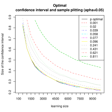
Figure 1: Upperbounds for cross-validation procedures with different splitting

5 Appendices

5.1 Notations and definitions

We recall the main notations and definitions.

Name	Notation	Definition
Generalisation error	$\widetilde{R}_{n}$	$\mathbb{E}_{P}[L(Y,\phi(X,\mathcal{D}_{n}))\mid\mathcal{D}_{n}]$
Resubstitution estimate	$\widehat{R}_{n}$	$\frac{1}{n}\sum_{i=1}^{n}L(Y_{i},\phi_{n}(X_{i},\mathcal{D}_{n}))$
Cross-validation estimate	$\widehat{R}_{CV}$	$\mathbb{E}_{V_{n}^{tr}}\hat{R}_{V_{n}^{ts}}(\phi_{V_{n}^{tr}})$
Cross-validation risk	$\bar{R}_{n(1-p)}$	$\mathbb{E}_{V_{n}^{tr}}R(\phi_{V_{n}^{tr}})$
Optimal error	$R_{opt}$	$\inf_{\phi\in\mathcal{C}}R(\phi)$

Table 1: Main notations

5.2 Proofs

We recall three very useful results. The first one, due to Hoeffding (1963), bounds the difference between the empirical mean and the expected value. The second one, due to Vapnik et al. (1971) , bounds the supremum over the class of predictors of the difference between the training error and the generalization error. The last one is called the bounded differences inequality McDiarmid (1989) .

Theorem 5.1 (Hoeffding (1963))

Let $X_{1,\ldots,}X_{n}$ independent random variables in $[a_{i},b_{i}]$. Then for all $\varepsilon>0,$

$$\mathbb{P}(\sum X_{i}-\mathbb{E}(\sum X_{i})\geq n\mathbb{\varepsilon})\leq e^{-\frac{2\varepsilon^{2}}{\sum_{i}(b_{i-}a_{i})^{2}}}$$

Theorem 5.2 (Vapnik et al. (1971))

Let $\mathcal{C}$ a class of predictors with finite VC-dimension and $L$ a loss function bounded by $1$. Then for all $\varepsilon>0,$

$$\mathbb{P}(\sup_{\phi\in\mathcal{C}}(\widehat{R}_{n}(\phi)-L(\phi))\geq\varepsilon)\leq c(n,V_{\mathcal{C}})e^{-\frac{\varepsilon^{2}}{2\sigma(n)^{2}}}$$

with $c(n,V_{\mathcal{C}})=2\mathcal{S}(2n,\mathcal{C}$)$\leq 2(2n+1)^{V_{\mathcal{C}}}$ and if $n\geq V_{\mathcal{C}},$ $2\mathcal{S}(2n,\mathcal{C}$)$\leq 2(\frac{2ne}{V_{\mathcal{C}}})^{V_{\mathcal{C}}}$ and $\sigma(n)^{2}=\frac{4}{n}$

Theorem 5.3 (McDiarmid)

Let $X_{1,\ldots,}X_{n}$ be independent random variables taking values in a sample $\mathcal{X}$, and assume that $f:\mathcal{X}^{n}\rightarrow\mathcal{R}$ satisfies

$$\forall i,\sup_{\begin{subarray}{c}x_{1},\ldots,x_{i},\ldots,x_{n}\\ x_{i}^{{}^{\prime}}\end{subarray}}|f(x_{1},...,x_{n})-f(x_{1},...,x_{i^{\prime}},...,x_{n})|\leq c_{i}.$$

Then, for all $\varepsilon>0,$

$$\mathbb{P(}f(X_{1},...,X_{n})-\mathbb{E}f(X_{1},...,X_{n})\geq\varepsilon)\leq e^{-\frac{2\varepsilon^{2}}{\sum_{i}c_{i}^{2}}}.$$

5.2.1 Proof of lemma 4.1

First, notice that

$$\mathbb{P(E}_{V_{n}^{tr}}\sup_{\phi\in\mathcal{C}}(\widehat{R}_{V_{n}^{tr}}(\phi)-R(\phi))-\mathbb{EE}_{V_{n}^{tr}}\sup_{\phi\in\mathcal{C}}(\widehat{R}_{V_{n}^{tr}}(\phi)-R(\phi))\geq\varepsilon)\leq e^{-2n\varepsilon^{2}},$$

using McDiarmid’s inequality by setting $f(X_{1},\ldots,X_{n})=\mathbb{E}_{V_{n}^{tr}}\sup_{\phi\in\mathcal{C}}(\widehat{R}_{V_{n}^{tr}}(\phi)-R(\phi))$ and since for all $i$,

$$\sup_{\begin{subarray}{c}x_{1},\ldots,x_{i},\ldots,x_{n}\\ x_{i}^{{}^{\prime}}\end{subarray}}|\mathbb{E}_{V_{n}^{tr}}\sup_{\phi\in\mathcal{C}}(\widehat{R}_{V_{n}^{tr}}(\phi)-R(\phi))-\mathbb{E}_{V_{n}^{tr}}\sup_{\phi\in\mathcal{C}}(\widehat{R}_{V_{n}^{tr}}^{{}^{\prime}}(\phi)-R(\phi))|$$

$$=\sup_{\begin{subarray}{c}x_{1},\ldots,x_{i},\ldots,x_{n}\\ x_{i}^{{}^{\prime}}\end{subarray}}\left|\mathbb{E}_{V_{n}^{tr}}\left[\sup_{\phi\in\mathcal{C}}(\widehat{R}_{V_{n}^{tr}}(\phi)-R(\phi))-\sup_{\phi\in\mathcal{C}}(\widehat{R}_{V_{n}^{tr}}^{{}^{\prime}}(\phi)-R(\phi))\right]\right|$$

$$\leq\sup_{\begin{subarray}{c}x_{1},\ldots,x_{i},\ldots,x_{n}\\ x_{i}^{{}^{\prime}}\end{subarray}}\mathbb{E}_{V_{n}^{tr}}\left|\sup_{\phi\in\mathcal{C}}(\widehat{R}_{V_{n}^{tr}}(\phi)-R(\phi))-\sup_{\phi\in\mathcal{C}}(\widehat{R}_{V_{n}^{tr}}^{{}^{\prime}}(\phi)-R(\phi))\right|$$

by Jensen’s inequality

$$\leq\sup_{\begin{subarray}{c}x_{1},\ldots,x_{i},\ldots,x_{n}\\ x_{i}^{{}^{\prime}}\end{subarray}}\mathbb{E}_{V_{n}^{tr}}\sup_{\phi\in\mathcal{C}}|\widehat{R}_{V_{n}^{tr}}(\phi)-\widehat{R}_{V_{n}^{tr}}^{{}^{\prime}}(\phi)|$$

$$\text{since }|\sup f-\sup g|\leq\sup|f-g|$$

$$\leq\frac{1}{n}.$$

Indeed, if we note $Q$ the number of elements in the sum $\mathbb{E}_{V_{n}^{tr}}$, the number of changes is lower than $\leq\frac{1}{Q}(\frac{1}{n(1-p_{n})}\text{multiplied by the number of times }i^{\prime}\text{ in the learning sample})$ that is $\frac{1}{Q}(\frac{1}{n(1-p_{n})}Q(1-p_{n}))=\frac{1}{n}$

Furthermore, we have

$$\mathbb{EE}_{V_{n}^{tr}}\sup_{\phi\in\mathcal{C}}(\widehat{R}_{V_{n}^{tr}}(\phi)-R(\phi)) =\mathbb{E}\sup_{\phi\in\mathcal{C}}(\widehat{R}_{\mathbf{v}_{n}^{tr}}(\phi)-R(\phi))$$

$$\text{with }\mathbf{v}_{n}^{tr}\text{ a fixed vector}$$

$$\leq\sqrt{\frac{2\ln(\mathcal{S}(2n(1-p_{n}),\mathcal{C})}{n(1-p_{n})}.}$$

by Vapnik-Chernovenkis’s inequality.

Thus, if we denote $\Pr\mathbb{(E}_{V_{n}^{tr}}\sup_{\phi\in\mathcal{C}}(\widehat{R}_{V_{n}^{tr}}(\phi)-R(\phi))\geq\varepsilon)$ by $P_{1}$ it leads to

$$P_{1}= \Pr\mathbb{(E}_{V_{n}^{tr}}\sup_{\phi\in\mathcal{C}}(\widehat{R}_{V_{n}^{tr}}(\phi)-R(\phi))-\mathbb{EE}_{V_{n}^{tr}}\sup_{\phi\in\mathcal{C}}(\widehat{R}_{V_{n}^{tr}}(\phi)-R(\phi))$$

$$\qquad\geq\varepsilon-\mathbb{EE}_{V_{n}^{tr}}\sup_{\phi\in\mathcal{C}}(\widehat{R}_{V_{n}^{tr}}(\phi)-R(\phi)).$$

Then, using the two previous inequalities

$$P_{1}\leq \Pr\mathbb{(E}_{V_{n}^{tr}}\sup_{\phi\in\mathcal{C}}(\widehat{R}_{V_{n}^{tr}}(\phi)-R(\phi))-\mathbb{EE}_{V_{n}^{tr}}\sup_{\phi\in\mathcal{C}}(\widehat{R}_{V_{n}^{tr}}(\phi)-R(\phi))$$

$$\qquad\geq\varepsilon-\sqrt{\frac{2\ln(\mathcal{S}(2n(1-p_{n}),\mathcal{C})}{n(1-p_{n})}}).$$

Since $2(u-v)^{2}\geq u^{2}-2v^{2}$, it follows

$$P_{1}\leq \exp(-2n(\varepsilon-\sqrt{\frac{2\ln(\mathcal{S}(2n(1-p_{n}),\mathcal{C})}{n(1-p_{n})}})^{2})\leq\exp(-n(\varepsilon^{2}-\frac{4\ln(\mathcal{S}(2n(1-p_{n}),\mathcal{C})}{n(1-p_{n})})))$$

$$\leq \mathcal{S}(2n(1-p_{n}),\mathcal{C})^{4/(1-p_{n})}\exp(-n\varepsilon^{2}).$$

$\Box$

5.2.2 Proof of lemma 4.1

Recall that $\widehat{R}_{CV}=\mathbb{E}_{V_{n}^{tr}}\widehat{R}_{{}_{V_{n}^{ts}}}(\phi_{V_{n}^{tr}})$

But by definition of $\phi_{n}$, we have $\widehat{R}_{n}(\phi_{n})\leq\widehat{R}_{n}(\phi_{V_{n}^{tr}})$.

It follows that $\frac{1}{n}(np_{n}\widehat{R}_{{}_{V_{n}^{ts}}}(\phi_{n})+\sum_{i\in V_{n}^{tr}}L(Y_{i,}\phi_{n}(X_{i}))\leq\frac{1}{n}(np_{n}\widehat{R}_{{}_{V_{n}^{ts}}}(\phi_{V_{n}^{tr}})\quad+\sum_{i\in V_{n}^{tr}}L(Y_{i,}\phi_{V_{n}^{tr}}(X_{i})).$

Thus, since $\sum_{i\in V_{n}^{tr}}L(Y_{i,}\phi_{n}(X_{i}))\geq\sum_{i\in V_{n}^{tr}}L(Y_{i,}\phi_{V_{n}^{tr}}(X_{i}))$ by definition of $\phi_{V_{n}^{tr}}$, we have $\widehat{R}_{{}_{V_{n}^{ts}}}(\phi_{n})\leq\widehat{R}_{{}_{V_{n}^{ts}}}(\phi_{V_{n}^{tr}}).$

From this, we deduce $\widehat{R}_{CV}=\mathbb{E}_{V_{n}^{tr}}\widehat{R}_{{}_{V_{n}^{ts}}}(\phi_{V_{n}^{tr}})\geq\mathbb{E}_{V_{n}^{tr}}\widehat{R}_{{}_{V_{n}^{ts}}}(\phi_{n})=\widehat{R}_{n}.$

$\Box$

5.2.3 Proof. of lemma 4.4

$$\forall\varepsilon>0,\mathbb{P}(X\geq\varepsilon)\leq\mathbb{P}(X_{+}\geq\varepsilon)\leq\frac{\mathbb{E}X_{+}}{\varepsilon}=\frac{\mathbb{E}X_{\_}}{\varepsilon}=\frac{\int_{0}^{1}\mathbb{P}(X_{-}\geq x)dx}{\varepsilon}=\frac{\int_{0}^{1}\mathbb{P}(X\leq-x)dx}{\varepsilon}.$$

$\Box$

5.2.4 Proof. of lemma 4.6

First, suppose that $q>1$ and notice that

$$\begin{array}[]{rcl}\mathbb{E}{Y_{+}}^{q}&=&\int_{0}^{\infty}qy^{q-1}\mathbb{P}(Y_{+}>y)dy\\ &=&q\int_{0}^{\infty}y^{q-1}\mathbb{P}(Y>y)dy.\end{array}$$

We thus deduce that because of the subgaussian inequality:

$$\begin{array}[]{rcl}\mathbb{E}{Y_{+}}^{q}&\leq&q\int_{0}^{\sigma\sqrt{4\ln(c)}}y^{q-1}dy+q\int_{\sigma\sqrt{4\ln(c)}}^{\infty}cy^{q-1}e^{-\frac{y^{2}}{2\sigma^{2}}}dy.\end{array}$$

Then, with $\mathcal{N}$ a standard normal:

$$\begin{array}[]{rcl}\mathbb{E}{Y_{+}}^{q}&\leq&(\sigma\sqrt{4\ln(c)})^{q}+qc\int_{\sigma\sqrt{4\ln(c)}}^{\infty}y^{q-1}e^{-\frac{y^{2}}{2\sigma^{2}}}dy\\ &\leq&(\sigma\sqrt{4\ln(c)})^{q}+qc\sqrt{2\pi}\sigma\mathbb{E}((\sigma\mathcal{N})^{q-1}1_{(\sigma\sqrt{4\ln(c)}\leq\sigma\mathcal{N})}).\end{array}$$

This gives by Cauchy-Schwarz’s inequality:

$$\begin{array}[]{rcl}\mathbb{E}{Y_{+}}^{q}&\leq&(\sigma\sqrt{4\ln(c)})^{q}+qc\sqrt{2\pi}\sigma^{q}(\mathbb{E}\mathcal{N}^{2(q-1)}1_{0\leq\mathcal{N}})^{\frac{1}{2}}(\mathbb{P}(\sqrt{4\ln(c)}\leq\mathcal{N}))^{\frac{1}{2}}.\end{array}$$

It leads to, since $\mathbb{E}\mathcal{N}^{2p}=\frac{(2p)!}{2^{p}p!}$, and$\sqrt{4\ln(c)}\geq 1$,

$$\begin{array}[]{rcl}\mathbb{E}{Y_{+}}^{q}&\leq&(\sigma\sqrt{4\ln(c)})^{q}+(2\pi)^{1/4}qc\sigma^{q}(\mathbb{E}\mathcal{N}^{2(q-1)})^{\frac{1}{2}}(e^{-\frac{(2)\ln(c)}{2}})^{\frac{1}{2}}\\ &\leq&(\sigma\sqrt{4\ln(c)})^{q}+(2\pi)^{1/4}q\sigma^{q}(\frac{(2(q-1))!}{2^{(q-1)}(q-1)!})^{\frac{1}{2}}.\end{array}$$

We obtain, since $\sqrt{2\pi n}(\frac{n}{e})^{n}e^{\frac{1}{12n}}\leq n!\leq\sqrt{2\pi n}(\frac{n}{e})^{n}e^{\frac{1}{12n+1}}$,

$$\begin{array}[]{rcl}\mathbb{E}{Y_{+}}^{q}&\leq&(\sigma\sqrt{4\ln(c)})^{q}+(2\pi)^{1/4}q\sigma^{q}\left(\frac{\sqrt{2\pi 2(q-1)}(\frac{2(q-1)}{e})^{2(q-1)}e^{\frac{1}{24(q-1)+1}}}{2^{(q-1)}\sqrt{2\pi(q-1)}(\frac{(q-1)}{e})^{k(q-1)}e^{\frac{1}{12(q-1)}}}\right)^{\frac{1}{2}}\\ &\leq&(\sigma\sqrt{4\ln(c)})^{q}+(2\pi)^{1/4}q\sigma^{q}(\sqrt{2}(\frac{2(q-1)}{e})^{(q-1)}e^{\frac{1}{24(q-1)+1}-\frac{1}{12(q-1)}})^{\frac{1}{2}}\\ &\leq&(\sigma\sqrt{4\ln(c)})^{q}+(2\pi)^{1/4}q2^{\frac{1}{4}}\sigma^{q}(\frac{2(q-1)}{e})^{\frac{q-1}{2}}.\end{array}$$

Thus, since $(a+b)^{\frac{1}{q}}\leq a^{\frac{1}{q}}+b^{\frac{1}{q}},a,b\geq 0$:

$$\begin{array}[]{rcl}(\mathbb{E}{Y_{+}}^{q})^{\frac{1}{q}}&\leq&\left((\sigma\sqrt{4\ln(c)})^{q}+(2\pi)^{1/4}q2^{\frac{1}{4}}\sigma^{q}(\frac{2(q-1)}{e})^{\frac{q-1}{2}}\right)^{\frac{1}{q}}\\ &\leq&\left((\sigma\sqrt{4\ln(c)})^{q}\right)^{\frac{1}{q}}+\left((2\pi)^{1/4}q2^{\frac{1}{4}}\sigma^{q}(\frac{2(q-1)}{e})^{\frac{q-1}{2}}\right)^{\frac{1}{q}},\end{array}$$

which gives since $q^{\frac{1}{q}}\leq 3^{\frac{1}{3}},(\frac{2(q-1)}{e})^{\frac{q-1}{2q}}\leq(\frac{2q}{e})^{\frac{q-1}{2q}}\leq(\frac{2q}{e})^{\frac{q}{2q}}$ since $\frac{2q}{e}\geq 1$:

$$\begin{array}[]{rcl}(\mathbb{E}{Y_{+}}^{q})^{\frac{1}{q}}&\leq&\sigma\sqrt{4\ln(c)}+q^{\frac{1}{q}}((2\pi)^{1/4}2^{\frac{1}{4}})^{\frac{1}{q}}\sigma(\frac{2(q-1)}{e})^{\frac{q-1}{2q}}\\ &\leq&\sigma\sqrt{4\ln(c)}+3^{\frac{1}{3}}2^{\frac{1}{4}}\sigma(\frac{2q}{e})^{\frac{1}{2}}.\end{array}$$

$$\begin{array}[]{rcl}&\leq&\sigma\sqrt{4\ln(c)}+(2\pi)^{1/4}3^{\frac{1}{3}}2^{\frac{3}{4}}e^{-\frac{1}{2}}\sigma\sqrt{q}\\ &\leq&(\sigma\sqrt{4\ln(c)}+(2\pi)^{1/4}3^{\frac{1}{3}}2^{\frac{3}{4}}e^{-\frac{1}{2}}\sigma)\sqrt{q}\\ &\leq&\sqrt{\gamma q}.\end{array}$$

with $\gamma=(\sigma\sqrt{4\ln(c)}+(2\pi)^{1/4}3^{\frac{1}{3}}2^{\frac{3}{4}}e^{-\frac{1}{2}}\sigma)^{2}$

For $q=1$, notice that:

$$\begin{array}[]{rcl}(\mathbb{E}{Y_{+}}^{q})^{\frac{1}{q}}&\leq&\sigma\sqrt{4\ln(c)}+\frac{1}{2}\sigma\\ &\leq&\sqrt{\gamma q}.\end{array}$$

$\Box$

References

• Allen (1968) Allen, D. M. (1968) The relationship between variable selection and data augmentation and a method for prediction. Technometrics, 16, 125-127.
• Arlot (2007) Arlot, S. (2007). Model selection by resampling penalization. submitted to COLT.
• Bengio et al. (2004) Bengio, Y. and Grandvalet, Y. (2004). No Unbiased Estimator of the Variance of K-Fold Cross-Validation. Journal of Machine Learning Research 5, 1089-1105.
• Markatou et al. (2005) Biswas, S. Markatou, M., Tian, H., and Hripcsak, G. (2005). Analysis of Variance of Cross-Validation Estimators of the Generalization Error. Journal of Machine Learning Research, vol. 6, 1127-1168.
• Breiman et al. (1984) Breiman, L., Friedman, J.H., Olshen, R. and Stone, C.J. (1984). Classification and regression trees. The Wadsworth statistics probability series. Wadsworth International Group.
• Breiman et al. (1992) Breiman, L. and Spector, P. (1992). Submodel selection and evaluation in regression: The X-random case International Statistical Review, 60, 291-319.
• Blum et al. (1999) Blum, A., Kalai, A., and Langford, J. (1999). Beating the hold-out: Bounds for k-fold and progressive cross-validation. Proceedings of the International Conference on Computational Learning Theory.
• Bousquet et al. (2001) Bousquet, O. and Elisseef, A. (2001). Algorithmic stability and generalization performance In Advances in Neural Information Processing Systems 13: Proc. NIPS’2000.
• Bousquet et al. (2002) Bousquet, O. and Elisseef, A. (2002). Stability and generalization. Journal of Machine Learning Research, 2:499-526.
• Burman (1989) Burman, P. (1989). A comparative study of ordinary cross-validation, v-fold cross-validation and the repeated learning-testing methods. Biometrika, 76:503– 514.
• Devroye et al. (1996) Devroye, L., Gyorfi, L. and Lugosi, G. (1996). A Probabilistic Theory of Pattern Recognition. Number 31 in Applications of Mathematics. Springer.
• Devroye et al. (1979) Devroye, L. and Wagner, T. (1979). Distribution-free performance bounds for potential function rules. IEEE Trans. Inform. Theory, Vol.25, pp. 601-604.
• Devroye et al. (1979) Devroye, L. and Wagner, T. (1979). Distribution-free inequalities for the deleted and holdout error estimates. IEEE Transactions on Information Theory, Vol.25(5), pp. 601-604.
• Dudoit et al. (2003) Dudoit, S. and Van Der Laan, M.J. (2003). Asymptotics of cross-validated risk estimation in model selection and performance assessment. Technical Report 126, Division of Biostatistics, University of California, Berkeley.
• Dudoit et al. (2004) Dudoit, S., van der Laan, M.J., Keles, S., Molinaro, A.M. , Sinisi, S.E. and Teng, S.L. (2004). Loss-based estimation with cross-validation: Applications to microarray data analysis. SIGKDD Explorations, Microarray Data Mining Special Issue.
• Van Der Laan et al. (2004) Van Der Laan, M.J., Dudoit, S. and Van der Vaart, A. (2004),The cross-validated adaptive epsilon-net estimator, Statistics and Decisions, 24 373-395.
• Geisser (1975) Geisser, S. (1975). The predictive sample reuse method with applications. Journal of the American Statistical Association, 70:320–328.
• Györfi et al. (2002) Györfi,L. Kohler, M. and Krzyzak, M. and Walk, H. (2002a). A distribution-free theory of nonparametric regression. Springer-Verlag, New York.
• Hastie et al. (2001) Hastie, T., Tibshirani, R. and Friedman, J.H. (2001). The Elements of Statistical Learning: Data Mining, Inference, and Prediction. Springer-Verlag.
• Hoeffding (1963) Hoeffding, W. (1963). Probability inequalities for sums of bounded random variables. Journal of the American Statistical Association, 58, 13?30.
• Holden (1996a) Holden, S.B. (1996). Cross-validation and the PAC learning model. Research Note RN/96/64, Dept. of CS, Univ. College, London.
• Holden (1996b) Holden, S.B. (1996). PAC-like upper bounds for the sample complexity of leave-one-out cross validation. In Proceedings of the Ninth Annual ACM Workshop on Computational Learning Theory, pages 41 50.
• Kearns et al. (1999) Kearns, M. and Ron, D. (1999). Algorithmic stability and sanity-check bounds for leave-one-out cross-validation. Neural Computation, 11:1427 1453.
• Kearns et al. (1995) Kearns, M. (1995). A bound on the error of cross validation, with consequences for the training-test split. In Advances in Neural Information Processing Systems 8. The MIT Press.
• Kearns et al. (1995) Kearns, M. J., Mansour, Y., Ng, A. and Ron, D. (1995). An experimental and theoretical comparison of model selection methods. In Proceedings of the Eighth Annual ACM Workshop on Computational Learning Theory, pages 21 30. To Appear in Machine Learning, COLT95 Special Issue.
• Kutin (2002) Kutin, S. (2002). Extensions to McDiarmid’s inequality when differences are bounded with high probability. Technical report, Department of Computer Science, The University of Chicago. In preparation.
• Kutin et al. (2002) Kutin, S. and Niyogi, P. (2002). Almost-everywhere algorithmic stability and generalization error. Uncertainty in Artificial Intelligence (UAI), August 2002, Edmonton, Canada.
• Lachenbruch et al. (1968) Lachenbruch, P.A. and Mickey, M. (1968). Estimation of error rates in discriminant analysis. TechnometricsLM68 Estimation of error rates in discriminant analysis. Technometrics, 10, 1-11.
• Li (1987) Li, K-C. (1987). Asymptotic optimality for cp, cl, cross-validation and generalized cross-validation: Discrete index sample. Annals of Statistics, 15:958–975.
• Lugosi (2003) Lugosi, G. (2003). Concentration-of-measure inequalities presented at the Machine Learning Summer School 2003, Australian National University, Canberra,
• McCarthy (1976) McCarthy, P. J. (1976). The use of balanced half-sample replication in crossvalidation studies. Journal of the American Statistical Association, 71: 596–604.
• McDiarmid (1989) McDiarmid, C. (1989). On the method of bounded differences. In Surveys in combinatorics, 1989 (Norwich, 1989), pages 148 188. Cambridge Univ. Press, Cambridge.
• McDiarmid (1998) McDiarmid, C. (1998). Concentration. In Probabilistic Methods for Algorithmic Discrete Mathematics, pages 195 248. Springer, Berlin.
• Picard et al. (1984) Picard, R.R. and Cook, R.D..(1984). Cross-validation of regression models. Journal of the American Statistical Association, 79:575–583.
• Ripley (1996) Ripley, B. D. (1996). Pattern recognition and neural networks. Cambridge University Press, Cambridge, New York.
• Shao (1993) Shao, J. (1993). Linear model selection by cross-validation. Journal of the American Statistical Association, 88:486–494.
• Stone (1974) Stone, M. (1974). Cross-validatory choice and assessment of statistical predictions. Journal of the Royal Statistical Society B, 36, 111?147.
• Stone (1977) Stone, M. (1977).Asymptotics for and against cross-validation. Biometrika, 64, 29?35.
• Vapnik et al. (1971) Vapnik, V. and Chervonenkis, A. (1971). On the uniform convergence of relative frequencies of events to their probabilities. Theory of Probability and its Applications, 16, 264?280.
• Van Der Vaart (1996) Van der Vaart, A. W. and Wellner, J. (19936. Weak Convergence and Empirical Processes. Springer-Verlag, New York.
• Vapnik et al. (1971) Vapnik, V. N. and Chervonenkis, A. Y. (1971). On the uniform convergence of relative frequencies of events to their probabilities. Theory of Probability and its Applications, 16(2):264–280.
• Vapnik (1982) Vapnik, V. (1982). Estimation of Dependences Based on Empirical Data. Springer-Verlag.
• Vapnik (1995) Vapnik, V. (1995). The nature of statistical learning theory. Springer.
• Vapnik (1998) Vapnik, V. (1998). Statistical learning theory. John Wiley and Sons Inc., New York. A Wiley-Interscience Publication.
• Yang (2007) Yang, Y. (2007). Consistency of Cross Validation for Comparing Regression Procedures. Accepted by Annals of Statistics.
• Zhang (1993) Zhang, P. (1993). Model selection via multifold cross-validation. Annals of Statistics, 21:299–313.
• Zhang (2000) Zhang, T. (2001). A leave-one-out cross validation bound for kernel methods with applications in learning. 14th Annual Conference on Computational Learning Theory - Springer.