Discussion of “Riemann manifold Langevin and Hamiltonian Monte Carlo methods” by M. Girolami and B. Calderhead

Introduction

This technical report is the union of two contributions to the discussion of the Read Paper Riemann manifold Langevin and Hamiltonian Monte Carlo methods (Calderhead and Girolami, 2010), presented in front of the Royal Statistical Society on October 13^th 2010 and to appear in the Journal of the Royal Statistical Society Series B.

The first comment establishes a parallel and possible interactions with Adaptive Monte Carlo methods. The second comment exposes a detailed study of Riemannian Manifold Hamiltonian Monte Carlo (RMHMC) for a weakly identifiable model presenting a strong ridge in its geometry.

1 On Adaptive Monte Carlo – J. Cornebise and G. Peters

The utility of RMMALA and RMHMC methodology is its ability to adapt Markov chain proposals to the current state. Many articles design Adaptive Monte Carlo (MC) algorithms to learn efficient MCMC proposals, such as the special case of controlled MCMC, Haario et al. (2001) which utilizes a historically estimated global covariance for a Random Walk Metropolis Hastings (RWMH) algorithm. Similarly, Atchadé (2006) devised global adaptation in MALA. Surveys are provided in Atchadé et al. (2009), Andrieu and Thoms (2008) and Roberts and Rosenthal (2009).

When the proposal remains essentially unchanged regardless of the current Markov chain state, performance may be poor if the shape of the target distribution varies widely over the parameter space. A typical illustration involves the “banana-shaped” warped Gaussian (see comments by Cornebise and Bornn), ironically originally utilized to illustrate the strength of early Adaptive MC (Haario et al., 1999, Figure 1). This algorithm learned local geometry by estimating the covariance matrix based on a sliding window of past states. However, Haario et al. (2001, Appendix A) showed it could exhibit strong bias, perhaps connected to requirements of “diminishing adaptation” as studied in Andrieu and Moulines (2006). Recent locally adaptive algorithms satisfy this condition, e.g. State-dependent proposal scalings (Rosenthal, 2010, Section 3.4) fits a parametric family to the covariance as a function of the state, or the parameterized parameter space approach of Regional Adaptive Metropolis Algorithms (Roberts and Rosenthal, 2009, Section 5).

Riemannian approaches provide strong rationale for parameterizing the proposal covariance as a function of the state – without learning, when the FIM (or observed FIM) can be computed or estimated, (see comment by Doucet and Jacob). With unknown FIM, or to learn the optimal step size, it would be interesting to combine Riemannian Monte Carlo with adaption. A first step could involve a simplistic Riemann-inspired algorithm such as a centered RWMH via the (observed) FIM as the proposal covariance (Section 4.3.1 Marin and Robert, 2007, as used in) – equivalent to one step of RMMALA without drift.

An additional use of Riemannian MC could be within the MCMC step of Particle MCMC (Andrieu et al., 2010), where adaption was highly advantageous in the AdPMCMC algorithms of Peters et al. (2010).

Another interesting extension involves considering the stochastic approximation alternative approach, based on a curvature updating criterion of (Okabayashi and Geyer, 2010, Equation 10), for an adaptive line search. This was proposed as an alternative to MCMC-MLE of Geyer (1991) for complex dependence structures in exponential family models. In particular comparing properties of this curvature based condition based on local gradient information with adaptive RMMALA and RMHMC versions of the MCMC-MLE algorithms would be instructive.

Additionally, one may consider how to extend Riemannian MC to trans-dimensional MC such as reversible jump (Richardson and Green, 1997), for which adaptive extensions are rare (Green and Hastie, 2009, Section 4.2). We wonder how a geometric approach may be extended to efficiently explore disjoint unions of model subspaces as in Nevat et al. (2009).

Finally, an open question to the community: could such geometric tools be utilized in Approximate Bayesian Computation (Beaumont et al., 2009), e.g. to design the distance metric between summary statistics?

2 RMHMC for unidentifiable models – J. Cornebise and L. Bornn

In this comment we show how the proposed RMHMC method can be particularly useful in the case of strong geometric features such as ridges commonly occurring in nonidentifiable models. While it has been suggested to use tempering or adaptive methods to handle these ridges (Neal, 2001; Haario et al., 2001, e.g.), they remain a celebrated challenge for new Monte Carlo methods (Cornuet et al., 2009). We suspect that RMHMC, by exploiting the geometry of the surface to help make intelligent moves along the ridge, is a brilliant advance for nonidentifiability sampling issues.

Consider observations $y_{1},\dots,y_{n}\sim\mathcal{N}(\theta_{1}+\theta_{2}^{2},\sigma_{y}^{2})$. The parameters $\theta_{1}$ and $\theta_{2}$ are non-identifiable without any additional information beyond the observations: any values such that $\theta_{1}+\theta_{2}^{2}=c$ for some constant $c$ explain the data equally well. By imposing a prior distribution, $\theta_{1},\theta_{2}\sim\mathcal{N}(0,\sigma_{\theta}^{2})$, we create weak identifiability, namely decreased posterior probability for $c$ far from zero. Figure 1 shows the prior, likelihood, and ridge-like posterior for the model.

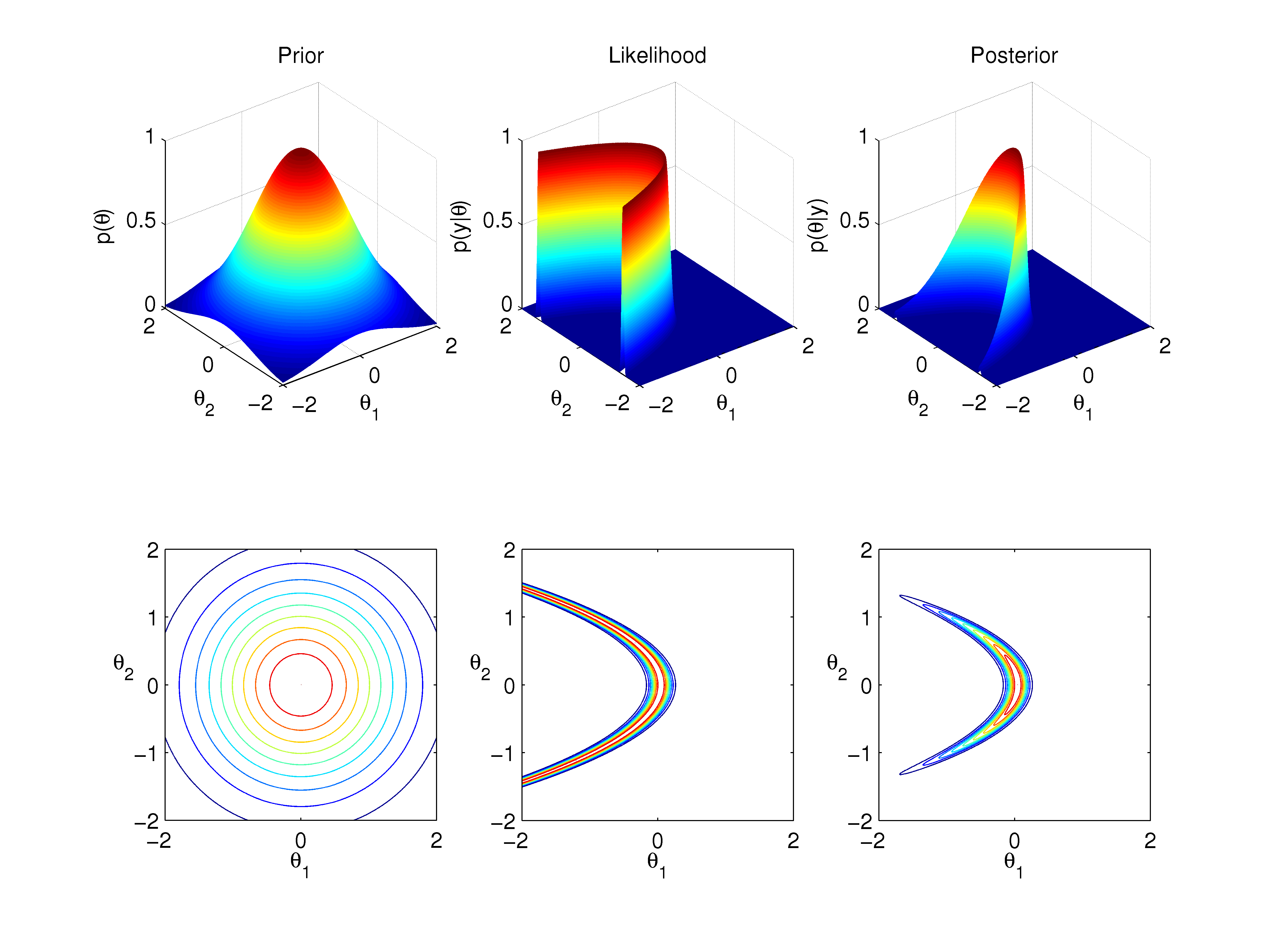
Figure 1: Prior, likelihood, and posterior for the warped bivariate Gaussian with $n=100$ values generated from the likelihood with parameter settings $\sigma_{\theta}=\sigma_{y}=1$. As the sample size increases and the prior becomes more diffuse, the posterior becomes less identifiable and the ridge in the posterior becomes stronger.

For this problem, we have

$$\bm{G}(\bm{\theta})=\left(\begin{array}[]{cc}\displaystyle\frac{n}{\sigma_{y}^{2}}+\frac{1}{\sigma_{\theta}^{2}}&\displaystyle\frac{2n\theta_{2}}{\sigma_{y}^{2}}\\[10.00002pt] \displaystyle\frac{2n\theta_{2}}{\sigma_{y}^{2}}&\displaystyle\frac{4n\theta_{2}^{2}}{\sigma_{y}^{2}}+\frac{1}{\sigma_{\theta}^{2}}\end{array}\right).$$

Figure 2 compares typical trajectories of both HMC and RMHMC, demonstrating the ability of RMHMC to follow the full length of the ridge.

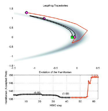
(a) RMHMC

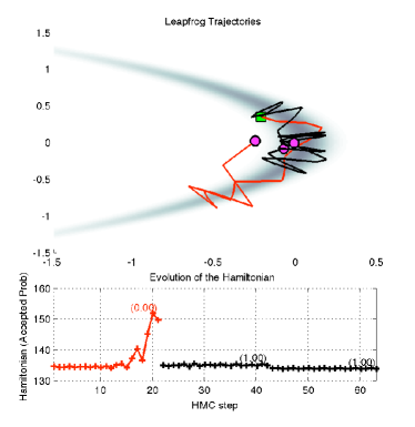
(b) HMC

Figure 2: Three typical consecutive trajectories of 20 leapfrog steps each, with step size of $0.1$, for the RMHMC and HMC algorithm, chosen to highlight two acceptances (black) and one rejection (red), representative of the approximately $65\%$ acceptance ratio for both HMC and RMHMC. We see that RMHMC is able to track the contours of the density and reach to the furthest tails of the ridge, adapting to the local geometry, whereas the spherical moves of HMC oscillate back and forth across the ridge.

HMC and RMHMC also differ in sensitivity to the step size. As described by Neal (2010), HMC suffers from the presence of a critical step size above which the error explodes, accumulating at each leapfrog step. In contrast, RMHMC occasionally exhibits a sudden jump in the Hamiltonian at one specific leapfrog step, followed by well-behaving steps (as seen in Figure 2.(a)). This is due to the possible divergence of the fixed point iterations (FPI) in the generalized leapfrog equations

$$\mathbf{p}\left(\tau+\frac{\varepsilon}{2}\right)=\mathbf{p}(\tau)-\frac{\varepsilon}{2}\nabla_{\bm{\theta}}H\left\{\bm{\theta}\left(\tau\right),\mathbf{p}\left(\tau+\frac{\varepsilon}{2}\right)\right\}$$ (16)

for given momentum $\mathbf{p}(\tau)$, parameter $\bm{\theta}(\tau)$ and step size $\varepsilon$. Figure 3 shows the probability of (16) having a solution $\mathbf{p}(\varepsilon/2)$ as a function of $\bm{\theta}(0)$, and of the derivative at the fixed point being “small enough” for the FPI to converge; the well-known sufficient theoretical threshold on the derivative (Fletcher, 1987, see e.g.) is $1$, but we conservatively chose $1.2$ based on typical successful runs.

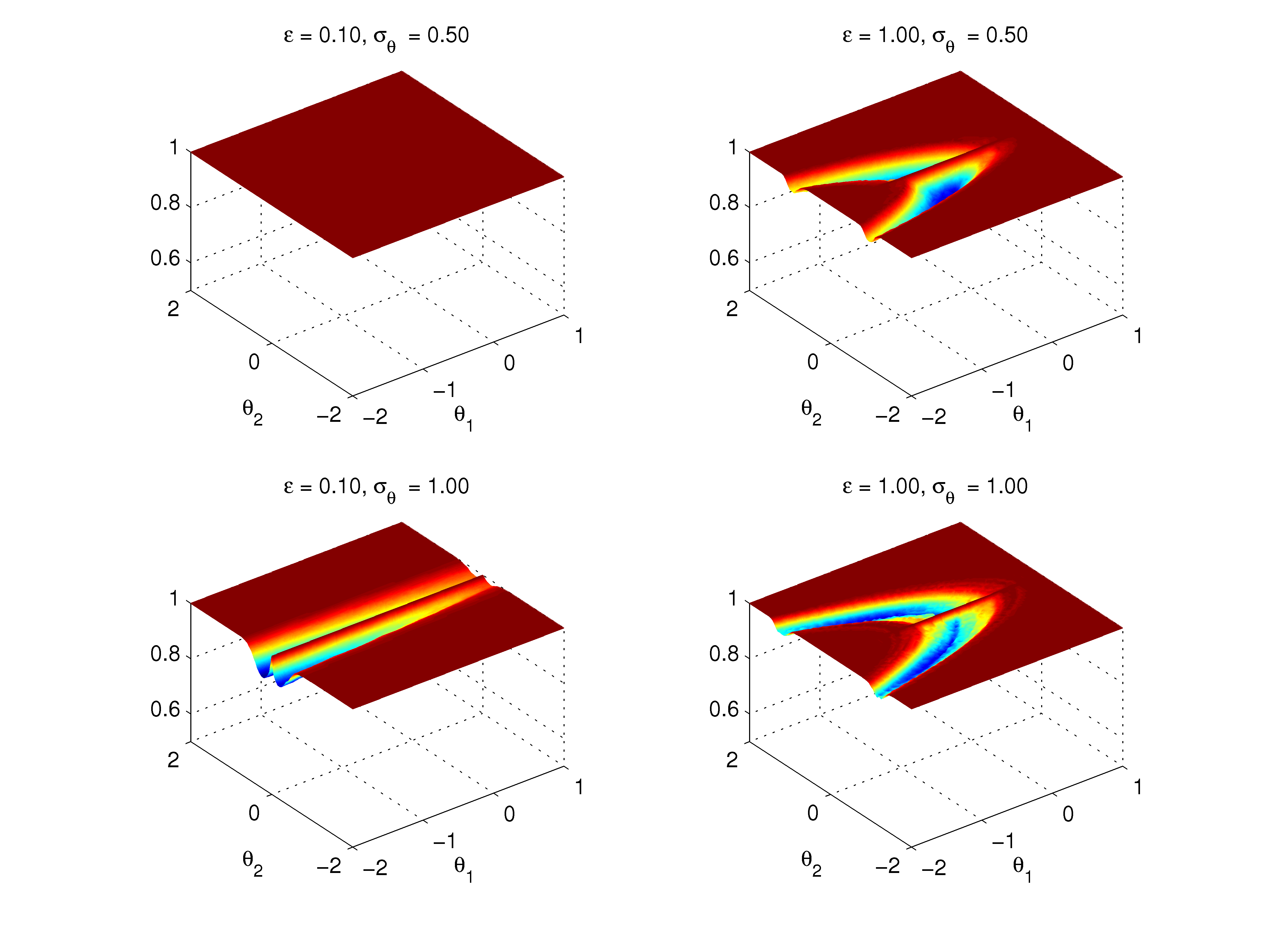
(a) Probability of existence of fixed point

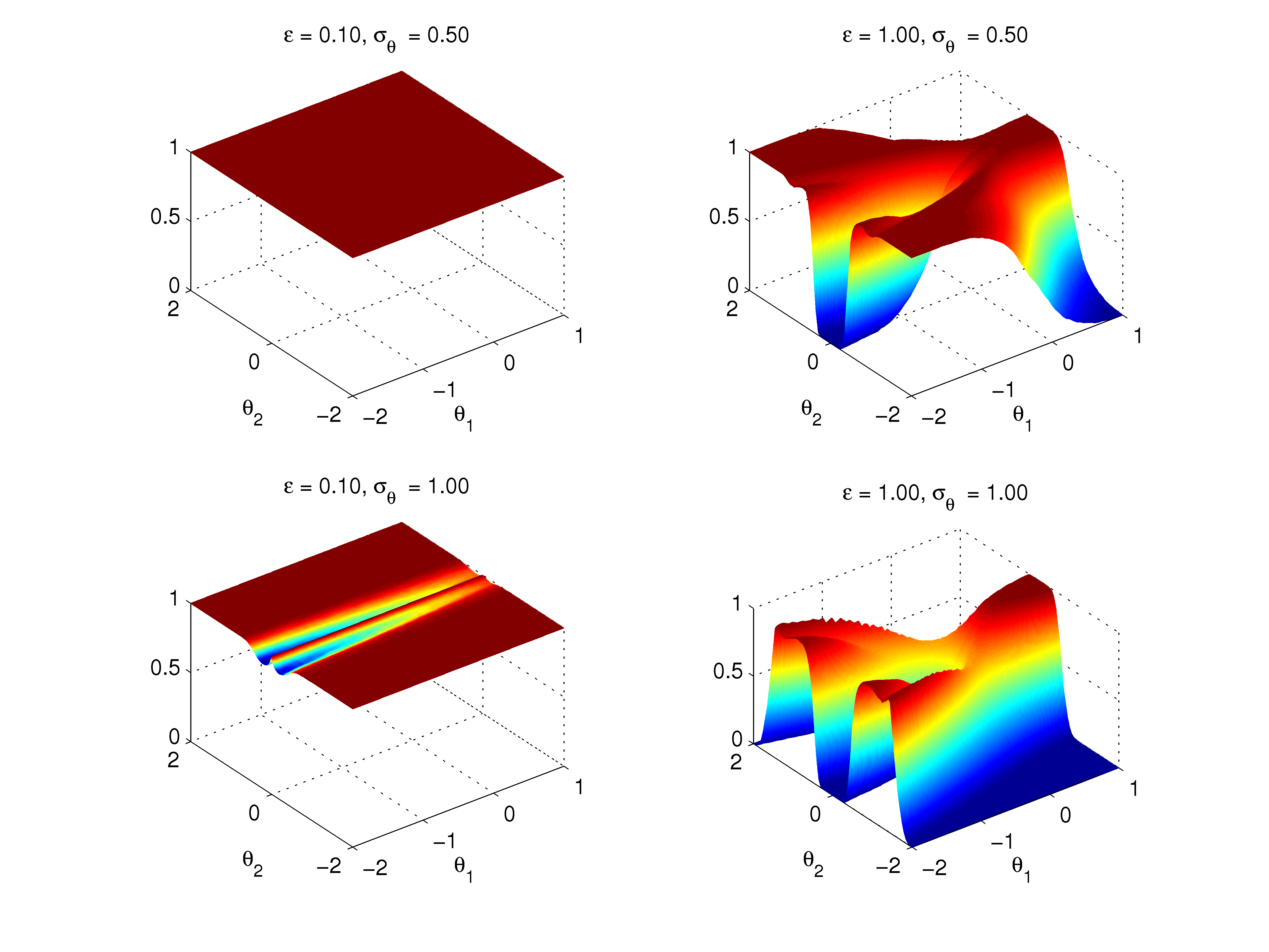
(b) Probability of existence of fixed point and of a derivative lower than 1.2

Figure 3: Probability of a single iteration of the generalized leapfrog (a) admitting a fixed point $\mathbf{p}\left(\frac{\varepsilon}{2}\right)$, (b) admitting a fixed point and having a small enough derivative at the fixed point for the FPI to converge. Both plotted as a function of starting point $\bm{\theta}(0)$. Shown for two step sizes $\varepsilon\in\{0.1,1.0\}$, and two prior distribution standard deviations $\sigma_{\theta}\in\{0.5,1.0\}$, i.e. varying levels of identifiability. The region of stability for FPI becomes much smaller as the step size increases and as identifiability decreases, even creating regions with null probability of convergence.

When the finite number of FPI diverges, the Hamiltonian explodes; however, subsequent steps may still admit a fixed point, and hence behave normally. Unsurprisingly, this behavior is much more likely to occur for larger step sizes.

While the regions of low probability can strongly decrease the mixing of the algorithm, they do not affect the theoretical convergence ensured by the rejection step. Far from being a downside, understanding this behavior can bring much practical insight when choosing the step size – possibly adapting it on-the-fly, when RMHMC already provides a clever way to adaptively devise the direction of the moves.

References

- Andrieu and Moulines (2006) C. Andrieu and É. Moulines. On the ergodicity properties of some adaptive MCMC algorithms. The Annals of Applied Probability, 16(3):1462–1505, 2006.
- Andrieu and Thoms (2008) C. Andrieu and J. Thoms. A tutorial on adaptive MCMC. Statistics and Computing, 18(4):343–373, 2008.
- Andrieu et al. (2010) C. Andrieu, A. Doucet, and R. Holenstein. Particle Markov chain Monte Carlo methods. J. R. Statis. Soc. B, 72(3):269–342, 2010.
- Atchadé et al. (2009) Y. Atchadé, G. Fort, E. Moulines, and P. Priouret. Adaptive Markov Chain Monte Carlo: Theory and Methods. Technical report, 2009.
- Atchadé (2006) Y.F. Atchadé. An adaptive version for the Metropolis adjusted Langevin algorithm with a truncated drift. Methodology and Computing in Applied Probability, 8(2):235–254, 2006.
- Beaumont et al. (2009) M.A. Beaumont, J.M. Cornuet, J.M. Marin, and C.P. Robert. Adaptive approximate bayesian computation. Biometrika, 96(4):983–990, 2009.
- Calderhead and Girolami (2010) B. Calderhead and M. Girolami. Riemann manifold Langevin and Hamiltonian Monte Carlo methods (with discussion). Journal of the Royal Statistical Society: Series B, to appear, 2010.
- Cornuet et al. (2009) J.M. Cornuet, J.M. Marin, A. Mira, and C. Robert. Adaptive multiple importance sampling. Technical report, ArXiV, 2009. URL \urlhttp://arxiv.org/abs/0907.1254.
- Fletcher (1987) R. Fletcher. Practical Methods of Optimization, second edition. 1987.
- Geyer (1991) C.J. Geyer. Markov chain Monte Carlo maximum likelihood. In Computing Science and Statistics: Proc. 23rd Symp. Interface, pages 156–163, 1991.
- Green and Hastie (2009) P.J. Green and D.I. Hastie. Reversible jump MCMC. Technical report, June 2009.
- Haario et al. (1999) H. Haario, E. Saksman, and J. Tamminen. Adaptive proposal distribution for random walk Metropolis algorithm. Computational Statistics, 14:375–395, 1999.
- Haario et al. (2001) H. Haario, E. Saksman, and J. Tamminen. An adaptive Metropolis algorithm. Bernoulli, 7(2):223–242, 2001.
- Marin and Robert (2007) J.M. Marin and C.P. Robert. Bayesian core: a practical approach to computational Bayesian statistics. Springer Verlag, 2007.
- Neal (2001) R.M. Neal. Annealed importance sampling. Statistics and Computing, 11(2):125–139, 2001.
- Neal (2010) R.M. Neal. MCMC using Hamiltonian dynamics. In S. Brooks, A. Gelman, G. Jones, and X.L. Meng, editors, Handbook of Markov Chain Monte Carlo. Chapman and Hall/CRC Press, 2010.
- Nevat et al. (2009) I. Nevat, G.W. Peters, and J. Yuan. Channel Estimation in OFDM Systems with Unknown Power Delay Profile using Trans-Dimensional MCMC via Stochastic Approximation. In Vehicular Technology Conference, 2009. VTC Spring 2009. IEEE 69th, pages 1–6. IEEE, 2009.
- Okabayashi and Geyer (2010) S. Okabayashi and C. J. Geyer. Long range search for maximum likelihood in exponential families. Technical report, 2010.
- Peters et al. (2010) G.W. Peters, G.R. Hosack, and K.R. Hayes. Ecological non-linear state space model selection via adaptive particle Markov chain Monte Carlo (AdPMCMC). Technical report, 2010.
- Richardson and Green (1997) S. Richardson and P.J. Green. On Bayesian analysis of mixtures with an unknown number of components (with discussion). Journal of the Royal Statistical Society: Series B, 59(4):731–792, 1997.
- Roberts and Rosenthal (2009) G.O. Roberts and J.S. Rosenthal. Examples of adaptive MCMC. Journal of Computational and Graphical Statistics, 18(2):349–367, 2009.
- Rosenthal (2010) J.S. Rosenthal. Optimal proposal distributions and adaptive MCMC. In S. Brooks, A. Gelman, G. Jones, and X.L. Meng, editors, Handbook of Markov Chain Monte Carlo. Chapman and Hall/CRC Press, 2010.