Spitzer observations of supernova remnants: ii@. Physical conditions and comparison with HH7 and HH54

Abstract

We have studied the shock-excited molecular regions associated with four supernova remnants (SNRs) — IC443C, W28, W44 and 3C391 — and two Herbig-Haro objects, HH7 and HH54, using $\it{Spitzer}$’s Infrared Spectrograph (IRS). The physical conditions within the observed areas (roughly $\sim~{}1^{{}^{\prime}}\times~{}1^{{}^{\prime}}$ in size) are inferred from spectroscopic data obtained from IRS and from the Short (SWS) and Long (LWS) Wavelength Spectrometers onboard the Infrared Space Observatory (ISO), together with photometric data from $\it{Spitzer}$’s Infrared Array Camera (IRAC).

Adopting a power-law distribution for the gas temperature in the observed region, with the mass of gas at temperature $T$ to $T+dT$ assumed proportional to $T^{-b}dT$, the H₂ S(0) to S(7) spectral line maps obtained with IRS were used to constrain the gas density, yielding estimated densities $n$(H₂) in the range of $\sim$ 2 – 4$\times 10^{3}$ cm^-3. The excitation of H₂ S(9) to S(12) and high-$J$ CO pure rotational lines, however, require environments several times denser. The inconsistency among the best-fit densities estimated from different species can be explained by density fluctuations within the observed regions. The best-fit power-law index $b$ is smaller than the value 3.8 predicted for a paraboloidal C-type bow shock, suggesting that the shock front has a “flatter” shape than that of a paraboloid. The best-fit parameters for SNRs and Herbig-Haro objects do not differ significantly between the two classes of sources, except that for the SNRs the ortho-to-para ratio (OPR) of hot gas ($T>$ 1000 K) is close to the LTE value 3, while for HH7 and HH54 even the hottest gas exhibits an OPR smaller than 3; we interpret this difference as resulting from environmental differences between these classes of source, molecular material near SNRs being subject to stronger photodissociation that results in faster para-to-ortho conversion. Finally, we mapped the physical parameters within the regions observed with IRS and found that the mid-lying H₂ emissions — S(3) to S(5) — tend to trace the hot component of the gas, while the intensities of S(6) and S(7) are more sensitive to the density of the gas compared to S(3) to S(5).

1 Introduction

Interstellar shocks generated by violent stellar activities, such as supernova explosions and protostellar outflows, have profound effects on the surrounding interstellar medium. Shocks propagating into dense molecular clouds can heat the gas to several hundred or several thousand Kelvin and produce rich spectra in the infrared spectral region. Fast shocks with speeds larger than 40 km s^-1 are usually dissociative; they destroy molecules and ionize atoms, generating strong atomic fine-structure emissions. On the other hand, most molecules survive in slow shocks. Heating excites various molecular species via collisional processes, causing the gas to glow. A large number of molecular line features have been observed in association with shock-affected areas, including cooling lines from H₂, CO, HD and H₂O. Due to its ability to reveal species that are difficult to observe within cold quiescent gas, a shock wave serves as a “searchlight” for the physical structure of molecular clouds.

Moreover, shocks alter the chemical composition of gas by driving many endothermic reactions, one of which is the conversion of para molecular hydrogen to ortho hydrogen. In previous studies, it has been found that many sources exhibit H₂ ortho-to-para ratio (hereafter OPR) markedly less than the equilibrium value $\sim 3$ (Neufeld et al. 1998; Cabrit, et al. 1999; Neufeld et al. 2006, hereafter N06; Neufeld et al. 2007, hereafter N07). Adopting a two component model containing a mixture of warm and hot gas, N06 and N07 found that for the sources we are studying in this paper – IC443C, W28, W44, 3C391, HH7 and HH54 – the OPR values in the warm gas component ($T\sim 300-600$ K) are 2.42, 0.93, 1.58, 0.65, 0.21 and 0.41–0.48 respectively. They proposed that the non-LTE OPR values obtained may correspond to the temperature at an earlier epoch, owing to the low efficiency of para-to-ortho conversion in non-dissociative shocks; this then can provide us useful information on the evolution timescale.

In this paper we investigate molecular shocks associated with four supernova remnants – IC443C, W28, W44 and 3C391 and two Herbig-Haro objects – HH7 and HH54. All six sources have extensive evidence for interaction with molecular clouds provided by multi-wavelength observations. A brief description of these sources is given below.

The four bright supernova remnant sources IC443, W28, W44 and 3C391 have provided excellent laboratories for the study of the interaction between SNR shocks and surrounding molecular gas. W28, W44 and 3C391 are prototypes of the “mixed-morphology” class, whose centrally concentrated X-ray morphologies contrast with the shell-like radio emission (Rho et al. 1994; Rho & Peter 1996; Rho & Peter 1998). The radio and X-ray morphology of IC443 also shows similarities to the mixed-morphology class, although with additional X-ray components. X-ray observations show the four remnants to be filled with a large amount of hot gas, with density $n~{}\sim$ 1 – 10 cm^-3 according to the radiative model of Harrus et al. (1997) and Chevalier (1999); this implicates an interaction with relatively dense environments — probably intercloud gas. More convincing evidence for the interaction with dense clouds arises directly from the detection of various excited molecules at longer wavelengths. As summarized by Reach et al. (2005) and N07 for each individual source in detail, this evidence includes broad line emissions in the millimeter-wave region; OH maser emission; near-infrared H₂ emission observed mainly by ground-based observatories; and mid-infrared emissions from various molecular species including H₂, CO, HD, H₂O, PAH, as well as atomic fine structure lines. Most of the mid-infrared spectra have been recently provided by the Infrared Space Observatory (ISO) and the Spitzer Space Telescope. All the evidence mentioned above has been obtained for all four SNRs.

IC443C is one of the four areas in IC443 marked by DeNoyer (1978), where bright condensations of HI have been seen. Near infrared observations reveal IC443 is evolving in a complex environment, with the northeast rim dominated by atomic fine structure lines including [FeII], [OI], etc. , and the southern ridge dominated by molecular line emissions, especially H₂ emissions (Rho et al. 2001). Rho et al. (2001) argued for the existence of fast shocks ($V_{s}$ $\sim$ 100 km s^-1) propagating in moderately dense gas ($n\sim$ 10 – 10³  cm^-3) within the northestern rim, and slow shocks ($V_{s}$ $\sim$ 30 km s^-1) in the denser ($n\sim$ 10⁴  cm^-3) southern part. IC443C coincides with the peak of the H₂ rovibrational emission in the southern rim.

HH7 is one of a chain of Herbig-Haro objects located in the star-forming region NGC 1333, separated by HH8 – 11 from the probable protostar SVS 13 (Strom, Vbra & Strom, 1979). It has been investigated extensively through optical and infrared observations as summarized by N06. HH7 exhibits a well defined bow shock in the infrared. Smith et al. (2003) studied the image of H₂ rovibrational emissions and found it can be well modeled by a paraboloidal bow shock with speed $\sim$ 55 km s^-1 and preshock density $\sim$ 8$\times$10³ cm^-3. HH54 is located at the edge of a star forming cloud Cha II (Hughes & Hartigan 1992) and consists of a complex of arcsecond scale bright knots (Graham & Hartigan 1988). The presence of warm molecular hydrogen was first reported by Sandell et al. (1987) and confirmed by Gredel (1994) with near-infrared observations. More infrared data come from observations with $\it{ISO}$ and $\it{Spitzer}$ (Cabrit et al. 1999; Neufeld et al. 1998; N06; Giannini et al. 2006) with the detection of several molecular features from H₂, HD, CO, H₂O, as well as many ionic lines.

The structure of this paper is as follows: the observational data we employed are discussed in Section 2; our analysis method is described in Section 3 and Appendix A along with the shock model; results for each individual source and a discussion are presented in Section 4 and 5; Section 6 serves as a brief summary of the paper.

2 Observations

In this paper we analyze the physical conditions in interstellar areas affected by interstellar shocks with the use of spectroscopic data obtained from the Infrared Spectrograph (IRS) on board Spitzer and two spectrometers on board ISO, as well as photometric data from the Spitzer’s Infrared Array Camera (IRAC).

2.1 IRS observations of H₂ and HD

Spanning a wide wavelength range from 5.2 to 37 microns, IRS on Spitzer provides access to pure rotational H₂ lines from $v$ = 0 – 0 S(0) to S(7) and a variety of fine structure lines including [Fe II], [S I], [Ne II] etc. Spectral maps of the six sources were obtained using the Short-Low (SL), Short-High (SH) and Long-High (LH) modules of IRS. Most of the data we employ here come from observations performed as part of the Cycle 2 General Observer Program, in which the IRS slit was stepped one-half of its width perpendicular to its long axis and 4/5 of its length parallel to the axis to map fields of size $\sim~{}1^{{}^{\prime}}\times~{}1^{{}^{\prime}}$. In Cycle 3, we obtained additional LH data with integration times a factor of 14 – 60 longer than those obtained in Cycle 2 for the H₂ S(0), HD R(3) and R(4) lines toward IC443C, HH7 and HH54, providing an improved signal-to-noise ratio. These Cycle 3 LH observations were carried out on 2007 April 22, 2007 November 11, 2007 May 1 and 3, and 2007 October 1 respectively for IC443C, HH54, and HH7. For the new observations $1^{{}^{\prime}}\times~{}1^{{}^{\prime}}$ regions were mapped by stepping IRS slit one-half its width perpendicular and 1/5 of its length parallel to its long axis. A detailed discussion of the data reduction procedures we adopted is given in N06 and N07.

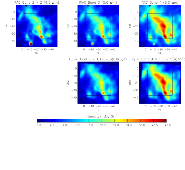
Figure 1: The upper panels show the three IRAC bands for IC443C at 4.5, 5.6, 8 $\mu$m and the lower panels show the IRS H₂ line contributions in 5.6 $\mu$m and 8$\mu$m bands calculated using equations (1) and (2) in NY08. The horizontal and vertical axes represent offsets in arcsec relative to $\alpha=6^{h}17^{m}44^{s}.2$ , $\delta=22^{\circ}21^{\prime}49^{\prime\prime}$ (J2000). IRAC band 3 (5.6 $\mu$m) is attributed mainly to H₂ S(6) and S(7) while IRAC band 4 (8 $\mu$m) is dominated by S(4) and S(5). We multiply the lower H₂ maps by a factor of 1.17 and 1.1 respectively to correct the “relative uncertainties” exiting between IRS and IRAC maps. The IRS H₂ and HD line intensities in table 1 are averaged over the region confined by the the solid line box. The cross in the northeast marks the center of the 80^′′ LWS beam observing the CO high-lying rotational lines.

In addition to H₂, the two HD rotational lines R(3) and R(4) detected in the IRS LH module toward IC443C, HH54 and HH7 provide us with an extra diagnostic of gas densities and the HD abundance (N06). A detailed discussion of our HD detections and abundance measurements will be presented in a future paper, which is in preparation. For each source, the line intensities for each H₂ and HD transition are listed in Table 1, averaged over the rectangular regions enclosed within the solid line boxes in Figure 1 – 6 to avoid pixels with poor signal-to-noise ratios.

2.2 IRAC observations and comparison with IRS

In addition to the IRS spectroscopic observations, photometric observations with IRAC on Spitzer may also help us in studying H₂. With four filters centered at 3.6, 4.5, 5.8 and 8 $\mu$m, IRAC covers a variety of rovibrational and pure rotational transitions of H₂ (Reach et al. 2006; NY08), providing access to higher excitation levels than those observable by IRS. More specifically, IRAC band 1 (covering $\sim$ 3.2 – 4.0$\mu$m) is sensitive to the $v$ = 1 – 0 O(5) to O(7) and $v$ = 0 – 0 S(13) - S(17) transitions of H₂; band 2 (3.8 – 5.1 $\mu$m) is sensitive to the $v$ = 0 – 0 S(9) to S(12) transitions; band 3 (4.9 to 6.5 $\mu$m) is sensitive to the $v$ = 0 – 0 S(6) to S(8) transitions; while band 4 (6.3 – 9.6 $\mu$m) is sensitive to the $v$ = 0 – 0 S(4) and S(5) transitions. The contributions of H₂ line emissions to each IRAC band are listed in Table 1 of NY08.

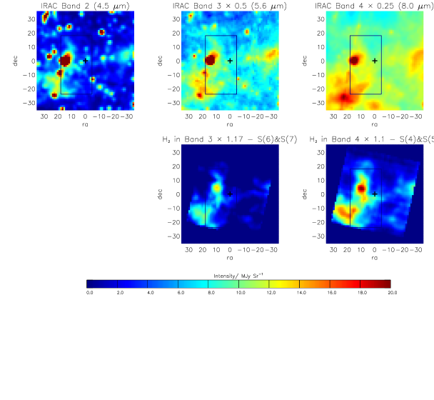
Figure 4: Similar as figure 1 but for 3C391. The (0,0) position is now at $\alpha=18^{h}49^{m}21.^{s}.9$, $\delta=-0^{\circ}57^{\prime}22^{\prime\prime}$ (J2000). The center of the $\it{ISO}$ observation(both SWS and LWS) coincides with the (0, 0) position in the maps.

After comparing the IRS H₂ spectral line maps pixel-by-pixel for IC443C with a IRAC map covering the same region obtained in Program 68, NY08 found that for this SNR source the IRAC band 3 (5.8 $\mu$m) and band 4 (8 $\mu$m) intensities are contributed almost entirely by H₂ $v$ = 0 – 0 S(4) to S(7) line emissions. The IRS spectrum for IC443C has been presented by N07, averaged over a Gaussian beam with HPBW $\sim$ 25” centered at $\alpha=6^{h}17^{m}44^{s}.2$ , $\delta=22^{\circ}21^{\prime}49^{\prime\prime}$ (J2000); this spectrum indicates that the H₂ pure rotational lines are the only detectable features within the two bandpasses. Moreover, according to the excitation model of NY08, H₂ S(8) emission accounts for only $\sim$3% of the observed band 3 intensity. Following the approach adopted in NY08, we present in Figure 1 a comparison between the IRAC band maps and the spatial distributions of corresponding band intensities contributed by IRS-observed H₂ lines only. These band intensities were calculated with the use of the IRAC spectral response functions presented by Fazio et al. (2004), in accord with equations (1) and (2) in NY08. We found that the IRS-derived 5.8 $\mu$m and 8 $\mu$m H₂ maps (based upon the H₂ line strengths) could be brought into excellent agreement with the observed IRAC band maps if multiplied by correction factors of 1.17 and 1.10 respectively. A more detailed comparison of the band intensities at each pixel is given in NY08’s Figure 4. The difference between the IRAC maps and maps derived from IRS H₂ emissions may be caused by different background measurements and systematic errors in flux calibration. For IC443C, most IRS-mapped regions are free of pollution from point sources.

According to the excitation model, the IRAC 4.5 $\mu$m band should also be attributed mainly to H₂ $v$ = 0 – 0 S(9) to S(12) line emissions. Significant contributions from other possible sources have been ruled out by ground-based spectroscopic observations for IC443C, including atomic hydrogen recombination lines (Br$\alpha$ at 4.05$\mu$m and Pf$\beta$ at 4.65 $\mu$m) (Burton et al. 1988) , [Fe II] fine structure lines and CO $v$ = 1 – 0 rovibrational transitions (Richter et al. 1995). Similarly, for IC443C, we expect the 3.6 $\mu$m channel to be dominated by H₂ $v$ = 1 – 0 rovibrational transitions (mainly $v$ = 1 – 0 O(5)). PAH continuum emissions, which are not detectable towards IC443C within the longer wavelength range in IRS, are expected to be unimportant in band 1. On the basis of the analysis above, IRAC band maps of IC443C provide another probe of the excitation conditions for H₂. Analysis of the IRS and IRAC maps for the other five sources will be given below. For cases where H₂ emission dominates, the IRAC band 2 brightness is used in conjunction with the spectroscopic data to constrain the excitation conditions for molecular hydrogen.

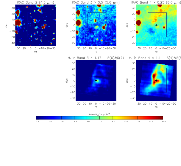
Figure 2: Similar as figure 1 but for W28. The (0, 0) position is now at $\alpha=18^{h}01^{m}52^{s}.3$ , $\delta=-23^{\circ}19^{\prime}25^{\prime\prime}$ (J2000). The center of the $\it{ISO}$ observation (both SWS and LWS) coincides with the (0,0) position in the maps.

In the Spitzer archive, two W28 IRAC maps in Program 20201, two W44 IRAC maps and two 3C391 IRAC maps in Program 186 are found to cover the same regions observed by IRS. IRAC maps for the same source are averaged to get better signal–to–noise ratio for each pixel. The comparison between the IRAC maps and the H₂ contributions for W28, W44 and 3C391 are shown in Figure 2 , 3 and 4, respectively. The IRS spectra, averaged over a Gaussian beam with HPBW $\sim$ 25” for each SNR source, are presented in N07. For all three SNRs, the PAH features are moderately strong within the IRAC 5.8$\mu$m and 8$\mu$m bands. Furthermore, all the IRAC maps are heavily polluted by point sources. For 3C391, the IRS map shows bright [Fe II] 5.34 $\mu$m emission from the western knot.

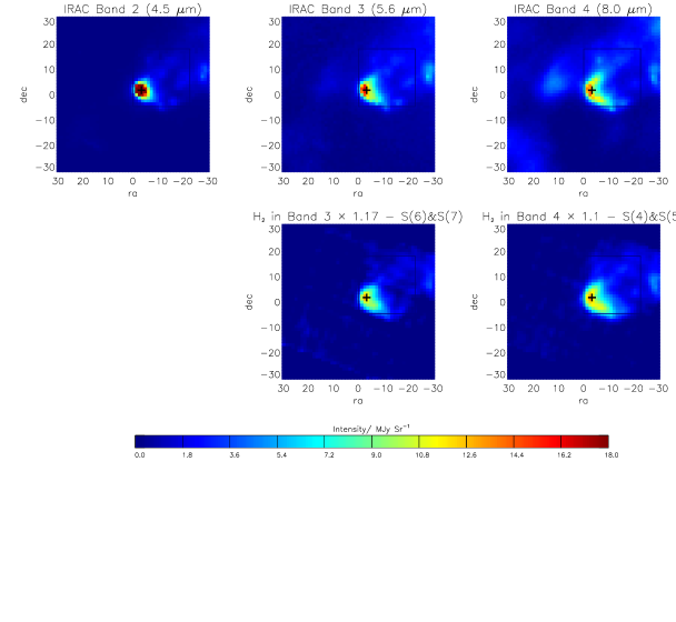
Figure 5: Similar as figure 1 but for HH7. The (0,0) position is now at $\alpha=3^{h}29^{m}8^{s}.6$ , $\delta=31^{\circ}15^{\prime}26^{\prime\prime}.8$ (J2000). The center of the 80^′′ LWS beam observing the CO lines is marked by the crosses.

The IRS spectra of HH7 and HH54 are shown in N06, which gives average spectra for 15” diameter circular apertures. We have extracted three HH7 IRAC maps obtained in Programs 6, 178 and 30516 from the $\it Spitzer$ archive. A comparison between the two sets of maps are shown in Figure 5. The IRAC band 4 (8$\mu$m) intensity for HH7 appears to come mainly from H₂ S(4) and S(5) line emissions; by contrast, the peak intensity in IRAC band 3 (5.8$\mu$m) is 50$\%$ stronger than that expected from the corresponding H₂ maps, which implies the presence of additional contributions from dust continuum emissions. The extraordinarily bright HH7 band 2 (4.5$\mu$m) intensity (compared with the brightness of band 3 and band 4) implies that it is probably dominated by continuum emission rather than H₂ emissions.

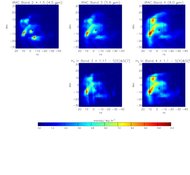
Figure 6: Similar as figure 1 but for HH54. The (0,0) position is now at $\alpha=12^{h}55^{m}51^{s}.5$ , $\delta=-76^{\circ}56^{\prime}19^{\prime\prime}.1$ (J2000). The center of the 40^′′ LWS beam observing the CO line emissions is marked by the crosses.

Two HH54 IRAC maps were obtained in Program 176. The similarity of the IRAC and IRS H₂ spectral images are apparent; see Figure 6. We have applied the same analysis method as in NY08 and found that, as for IC443C, the two IRAC bands for HH54 (5.8$\mu$m and 8$\mu$m) are mainly accounted for by H₂ emissions. It should be noted that N06 detected a weak [Fe II] fine structure line at 5.34 $\mu$m toward HH54, which should contribute less than 18$\%$ of the 5.8 $\mu$m band intensity for most positions in the map. The morphology of the HH54 4.5 $\mu$m band emission is similar to that of the IRS H₂ spectral line maps, though it is a little more clumpy, implying that the H₂ line emissions are also very important components within band 2. We are assuming here that for HH54, like IC443C, the IRAC 4.5 $\mu$m band (band 2) is also dominated by H₂ emissions, i.e. the contribution from other species is less than 25$\%$ in band 2, which is the typical error in the line intensity. Other possible contributors include atomic hydrogen recombination lines – Br$\alpha$ and Pf$\beta$ – which should be weak for molecular shocks, [Fe II] fine structure lines, and dust continuum emission. The possibility of strong CO v = 1 – 0 emission in the 4.5 $\mu$m band was shown to be unlikely by NY08. NY08 considered collisional excitation of CO v = 1 – 0 transitions by H and H₂ and found that even at a H/H₂ ratio $\sim 1$ and a high density with $n$(H${}_{2})=10^{6}$ cm^-3, the fractional contribution of CO emission to the 4.5 $\mu$m band is less than $20\%$. For gas with H/H₂ $\sim 10\%$ and $n$(H${}_{2})=10^{4}$ cm^-3, the fraction would be less than $2\%$.

2.3 Additional constraints imposed by ISO observations of CO and H₂

The two complementary spectrometers on ISO provide us with more molecular data for these shock-excited regions. The Long-Wavelength Spectrometer (LWS) is designed for spectroscopic observations in the range of 43 – 196.9 $\mu$m and covers many high-lying CO pure rotational transitions. The detection of CO emission with $J$ $>$ 14 in LWS observations has been reported for all six sources. Snell et al. (2005) presented observations of three CO lines, $J$ = 15 – 14, $J$ = 16 – 15, $J$ = 17 – 16, within the 80^′′ LWS beam centered on IC443C from the $\it{ISO}$ archive. In the LWS observations carried out by Reach & Rho (1998), four CO lines were detected toward 3C391, viz. $J$ = 14 – 13, $J$ = 15 – 14, $J$ = 16 – 15 and $J$ = 17 – 16. For W28, they detected only the CO $J$ = 15 – 14 and $J$ = 16 – 15 transitions. For W44, only the $J$ = 16 – 15 line could be identified. Molinari et al. (2000) observed several locations along the HH 7 – 11 flow and detected four CO rotational lines within the LWS beam on HH7: $J$= 14 – 13, $J$ = 15 – 14, $J$ = 16 – 15 and $J$ = 17 – 16. The LWS CO spectrum for HH54 was taken toward a position called HH54B, marked by the crosses in Figure 6. Six CO rotational features, $J$ = 14 – 13, $J$ = 15 – 14, $J$ = 16 – 15, $J$ = 17 – 16, $J$ = 18 – 17 and $J$ = 19 – 18, were reported by Nisini et al. (1996) and Liseau et al. (1996). With an improved Relative Spectral Response Function, Giannini et al. (2006) presented a new analysis of the spectra, leading to the detection of CO $J$ = 20 – 19. For these observations, the measured line fluxes had calibration uncertainties estimated to be up to $\sim$ 30$\%$. With larger critical densities of the order of 10⁷ cm³ , these CO high-lying rotational lines can provide sensitive diagnostics for probing density in these regions.

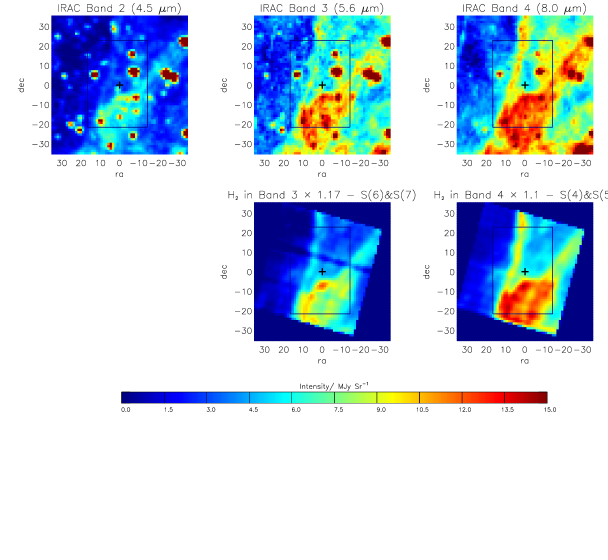
Figure 3: Similar as figure 1 but for W44. The (0,0) position is now at $\alpha=18^{h}56^{m}28^{s}.4$ , $\delta=01^{\circ}29^{\prime}59^{\prime\prime}$ (J2000). The center of the $\it{ISO}$ observation (both SWS and LWS) coincides with the (0, 0) position in the maps.

Besides the CO emissions, Reach and Rho (2001) obtained spectra of the H₂ S(9) and S(3) lines for W28, W44 and 3C391 within the $14^{\prime\prime}\times 20^{\prime\prime}$ aperture of the Short Wavelength Spectrometer (SWS) on $\it{ISO}$. The central positions of all these $\it{ISO}$ observations are marked by the crosses on Figures 1 – 6. For W28, W44 and 3C391 the LWS and SWS observations share the same beam centers and are consistent with the $(0,0)$ positions of the IRS maps. The measured H₂ S(9)/S(3) ratios are another valuable diagnostic tool and are used in our fits to constrain the best-fit parameters of the gas. The LWS measured CO line fluxes along with the 1 $\sigma$ errors and the SWS S(9)/S(3) ratios are all listed in Table 1.

3 Molecular Emission from C-type shocks

3.1 The Excitation Model

The H₂ emission spectrum is among the most important diagnostics needed to constrain conditions in shocked molecular gas as well as to distinguish between different shock models. Over the last several decades, it has been widely observed that the rotational diagrams of H₂ often exhibit positive curvatures. This kind of curvature can not be accounted for by extinction effects only, which affect the H₂ S(3) line much more strongly than the other rotational lines, and may imply the existence of a mixture of gas temperatures. N06 and N07 investigated the H₂ excitation diagrams for the six sources we are studying here, in which the molecular hydrogen emission was modeled with a combination of gas at two temperatures. In this paper, we adopt a power-law temperature distribution similar to that described by NY08, with the column density of gas at temperature between $T$ and $T$ + $dT$ assumed to be proportional to $T^{-b}$. Instead of the lower temperature limit $T_{min}$ = 300 K adopted by NY08, we extend it to 100 K here because warm gas at 100 – 300 K can contribute significantly to those low-lying H₂ emissions accessible to IRS, especially for v = 0 – 0 S(0) and S(1). This power-law distribution is consistent with the prediction from the bow-shaped C-shock model developed by Smith, Brand & Moorhouse (1991) (NY08). Smith, Brand & Moorhouse found that bow shocks can produce gas at a wide range of excitation temperatures and thus provide a way of explaining the H₂ line ratios observed for many sources, while planar shock models fail to reproduce the observed ratios.

Another interesting characteristic of the H₂ rotational diagrams lies in the zigzag pattern, corresponding to non-equilibrium H₂ ortho-to-para ratios. This phenomenon is especially notable for the five sources W28, W44, 3C391, HH7 and HH54 (N06; N07). With a closer look, it is quickly apparent that the zigzag tends to “diminish” for high–lying levels. Given the fact that low- and high-excitation lines are produced by different temperature components, N06 argued that the change in the degree of zigzag is caused by the strong temperature dependence of the para-to-ortho conversion efficiency. With this process dominated by collisions with atomic hydrogen in C-type shocks (Timmermann 1998; Wilgenbus et al., 2000), the current OPR is given by equation (1) in Neufeld et al. (2009; hereafter N09), as a function of initial ratio OPR₀, atomic hydrogen density n(H) and shock-heating period $\tau$. These three values along with the number and column density of H₂ — $n$(H₂) and $N$(H₂) — determine the H₂ emission spectrum.

3.2 Constraining the physical parameters

For an excitation model with the parameters discussed above, the molecular line intensities are easy to calculate if statistical equilibrium is achieved, which is an approximation widely adopted for modeling molecular emission in shocks. We have confirmed the validity of this approximation for transitions of the three species H₂, HD and CO accessible in the infrared observations mentioned in this paper (see Appendix A). The rate equations are then simplified as

$$\sum_{J^{\prime}}\left(C_{J^{\prime}\rightarrow J}+A_{J^{\prime}\rightarrow J}\right)f_{J^{\prime}}-f_{J}\cdot\sum_{J^{\prime}}\left(C_{J\rightarrow J^{\prime}}+A_{J\rightarrow J^{\prime}}\right)=0,$$ (1)

where $f_{J}$ represents the fractional population in state $J$, $A_{J^{\prime}\rightarrow J}$ is the rate of spontaneous decay from state $J^{\prime}$ to $J$, and $C_{J^{\prime}\rightarrow J}$ is the rate of collisionally-induced transitions from $J^{\prime}$ to $J$. We consider collisional excitation (de-excitation) and spontaneous decay processes only, and for H₂ and HD we neglected optical depth effects. For the H₂ collisional rate coefficients, we used data computed by Flower & Roueff (1999), Flower et al. (1998), Flower & Roueff (1998b) and Forrey et al. (1997). The rate coefficients for HD were adopted from Flower (1999), Roueff & Zeippen (1999) and Roueff & Flower (1999). For CO, we made use of collisional data from Flower (2001), Wernli et al. (2006) and Balakrishnan et al. (2002), together with the extrapolation presented by Schoier et al. (2005) for temperatures up to 2000 K and CO rotational states up to $J=40$. For cases where optical depth effects may become non-negligible, specifically for the CO transitions, we applied the large-velocity-gradient (LVG) approximation and multiplied the radiative transition part in equation (1) by a term $\beta$, which is called the escape probability for photons. Neufeld & Kaufman (1993) suggested an angle-averaged probability for planar shocks

$$\beta={1\over 1+3\tau_{s}}$$ (2)

where $\tau_{s}$ is the Sobolev optical depth. An average velocity gradient of 2 $\times 10^{-10}$ cm s^-1/cm and a $n$(CO)/$n$(H₂) abundance ratio of 5 $\times 10^{-5}$ are adopted in calculating the CO optical depth. We note however, that the optical thickness of CO affects these highly excited rotational states measured in LWS observations by less than 10%.

We have adopted two approaches to find the best-fit parameters in the shock model using a $\chi^{2}$ minimization method. In the first approach, we considered only the H₂ spectral lines S(0) – S(7) observed by IRS; while in the second approach we fitted all the available data, including the IRS H₂ intensities, the IRAC band 2 intensities – if dominated by high-lying H₂ rotational transitions (IC443C and HH54) – the HD R(3) & R(4) intensities, and the CO line fluxes obtained from the $\it{ISO}$ archive. We decided not to use the IRAC 3.6 $\mu$m band intensities, which are attributable to H₂ ro-vibrational emissions. The excitation of H₂ vibrational transitions, unlike the pure rotational lines we considered, is dominated by collisions by atomic hydrogen even with a small $n$(H)/$n$(H₂) ratio $\sim$ 3$\%$ (NY08). Since the collisional dissociation processes for molecular hydrogen are more efficient within the hotter component of the shocked gas, the dependence of the H₂ vibrational emission upon temperature will be more complicated than what our model describes. Thus, we exclude IRAC band 1 (3.6 $\mu$m) in the fitting to avoid it affecting our estimate of the best fit temperature distribution and density. For the other transitions mentioned above, the excitation processes should be always dominated by collisions with H₂ given the conditions in molecular shocks. In our calculation, we take into account collisional excitation by H₂ and helium. A helium abundance $n$(He)/$n$(H₂) of 0.2 is assumed. Errors introduced by neglecting collision with atomic hydrogen are largest for the CO lines and those high-lying H₂ transitions contributing to IRAC band 2, which are however still less than 15$\%$ given an average $n$(H)/$n$(H₂) ratio of 10$\%$ , which is the upper limit of the value for IC443C estimated by Burton et al. (1988) based on the Br$\gamma$ intensity.

4 Results

As mentioned in Section 3, we used two ways to derive the best-fit parameters. In the first approach, only IRS H₂ lines were considered. In the second approach, all available molecular data were included in the fitting process. In the case of IC443C and HH54, these data comprise the H₂ & HD line intensities observed by IRS, the IRAC band 2 intensity, and the CO line intensities observed by ISO/LWS. For W28, W44 and 3C391, we included the H₂ lines and SWS-measured S(9)/S(3) ratios. For HH7, only the IRS-observed H₂ and HD lines were used. We found that the uncertainties in the LWS-measured CO line intensities for W28, W44, 3C391 and HH7 are too large to provide useful information about the physical conditions in the gas.

To deredden the IC443C line fluxes, we originally tried the extinction correction with $A_{2.12\mu m}$ = 1.3 – 1.6 by Richter et al. (1995) and the R_V = 3.1 extinction curves from Weingartner & Draine (2001), which ended up with a S(3) intensity almost two times larger than expected given the other H₂ line intensities. Treating the extinction as a free parameter in our fit to the H₂ line intensities yielded an A_V close to zero. Thus, we applied no extinction correction for IC443C in the following calculations. For W28, we applied an extinction correction with E_B-V= 1 – 1.3 given by Long et al. (1991) derived from the [S II] line ratios. This value is also consistent with the estimate by Bohigas et al. (1983) who obtained E_B-V= 1.16. For W44, the absorbing column density along the line-of-sight to this region is estimated to be $\sim 2\times 10^{22}~{}$cm^-2 (Rho et al. 1994), corresponding to an A_V $\sim$ 10. For 3C391, Reach et al. (2002) suggested a visual extinction of A_V = 19 for the IRS-observed region, which is denser than other parts of the cloud, based upon an upper limit on the foreground column density of $(2-3.6)\times 10^{22}$ cm^-2 inferred from a spectral analysis of the X-ray data (Rho $\&$ Petre 1996). For HH7, we adopted E_J-K = 0.7, as estimated by Gredel (1996) for the neighboring source HH 8, and for HH54 we assumed A${}_{V}=1.64$, following Gredel (1994).

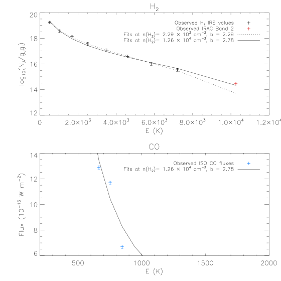
Figure 7: The upper panel shows best fits to IC443C H₂ rotational diagram and the lower panel represents fits to the CO excitation diagram. We adopted two different approaches in the fitting. The dotted line represents fits computed with the IRS H₂ lines S(0) to S(7) only and solid lines represent fits to all features including IRS H₂ and HD lines, IRAC band 2 (4.5 $\mu$m) emission, LWS CO fluxes $J$ = 15–14, $J$ = 16–15 and $J$ = 17–16. To show fit to IRAC band 2 (4.5 $\mu$m) , we assume that half of the band 2 intensity comes from H₂ S(9) and plot that false “S(9)” on the H₂ rotational diagram, represented by the red cross on the upper panel. The error bars for each line are plotted assuming 30% uncertainties for LWS CO fluxes and 25% for the rest.

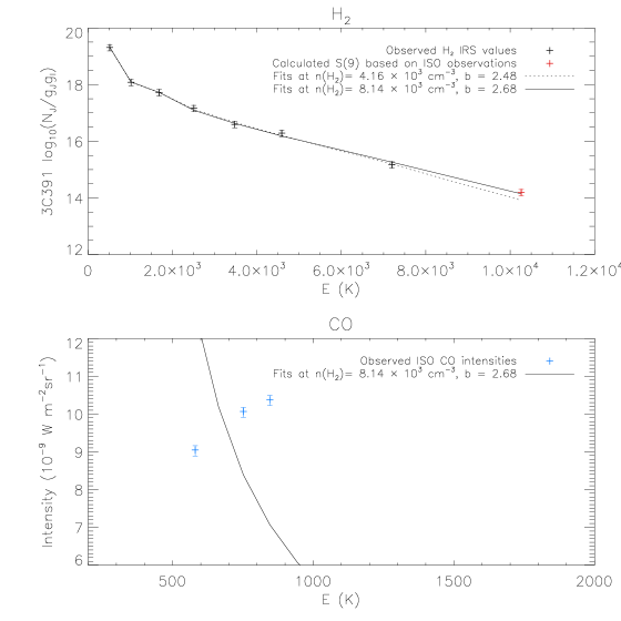
Figure 10: Same as Figure 7 but for 3C391. The H₂ S(6) line is not included as it cannot be measured reliably. Though fits to the CO rotational diagram is still shown in the lower panel, these CO fluxes observed in LWS observation, including $J$ = 14–13, $J=$ 15–14, $J=$ 16–15 and $J=$ 17–16, are excluded in our computation because of large uncertainties. Noted here the observed CO flux for $J=$ 15–14 is way above the range of the plot, which may result from unreliable measurement.

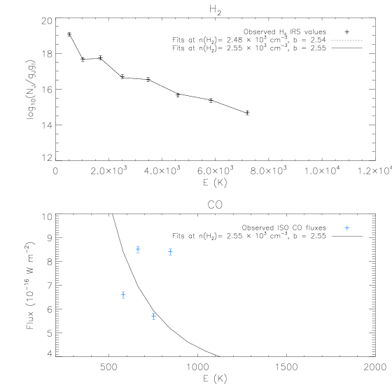
Figure 11: Same as Figure 7 but for HH7. Solid lines represent fits to IRS H₂ and HD lines. Since the two fits are very close the dotted and solid lines overlap. Though fits to the CO rotational diagram is still shown in the lower panel, the CO fluxes observed in LWS observation, including $J=14$–13, $J=$ 15–14, $J=16$–15 and $J=17$–16, are excluded in our computation due to large uncertainties.

The best fits to the H₂ and CO rotational diagrams are shown by the dotted lines (first approach) and solid lines (second approach) in Figures 7 to 12. In the case of H₂ S(9), we assumed an S(9)/S(3) line ratio equal to that measured by ISO/SWS for the sources W28, W44 and 3C391. For IC443C and HH54, we estimated the S(9) line intensity from the IRAC band 2 intensity, assuming one-half of the emission in that band to result from H₂ S(9), roughly consistent with the fractional contribution obtained by NY08 ($62\%$ for one specific excitation model with an assumed $b$ of 4.5 and $n$(H${}_{2})$ of $10^{6}~{}$ cm^-3 reported in their Table 1). Though the CO lines are excluded in the fits for 3C391 and HH7, the excitation diagrams of CO for these two sources were still presented in Figures 10 and 11. The best-fit parameters for each source are listed in Table 2. From this table, we can see that while the best-fit density determined from the H₂ pure rotational transitions alone is $\sim 2-4\times 10^{3}~{}$cm^-3, a value several times larger provides the best-fit to the complete data set including the H₂ S(9), IRAC band 2, HD and CO line intensities.

Although the IRS maps are smaller than the whole regions that contribute to the 80^′′ LWS beam, we can place an upper limit on the average CO abundance by comparing the H₂ line fluxes obtained in each entire IRS map with the CO fluxes obtained with LWS. This method yields the firm upper limits $n$(CO)/$n$(H₂) $<1.5\times 10^{-3}$ and $n$(CO)/$n$(H₂) $<5.5\times 10^{-4}$ for IC443C and HH54, respectively. If we assume the distribution of CO emission to be similar to that measured in IRAC band 2, we obtain rough estimates of the CO abundance of $\sim 3-5\times 10^{-5}$ for IC443C and $\sim 2-4\times 10^{-5}$ for HH54.

Errors in the fitted parameters are evaluated by plotting $\chi^{2}$ contours in multi-parameter spaces. The $\chi^{2}$ values are computed assuming a fractional uncertainty of 30$\%$ for the CO line fluxes and $25\%$ for all other line emissions. Figure 13 shows the $68.3\%$ and $95.4\%$ confidence regions in the $b$ – $n$(H₂) plane for all six sources, with dotted lines for fits with IRS H₂ lines only and solid lines for fits with all reliable data included (second approach discussed above). The elongated shape of the $\chi^{2}$ contours in the $b$ – $n$(H₂) plane arises because the two parameters are degenerate, as mentioned in N09, such that increasing the density or decreasing $b$ (which raises the fraction of hot gas) have a similar effect on the excitation of mid- and high-lying transitions considered in the calculation. For HH7, including the HD R(3) and R(4) lines in our calculation does not significantly change the best-fit parameters. The two sets of contour plots for HH7 almost overlap with each other, as shown in Figure 13; this is because within the banana-shaped region constrained by the H₂ emission, the HD R(3) to R(4) ratio is not a sensitive function of the gas density or the power-law index, $b$.

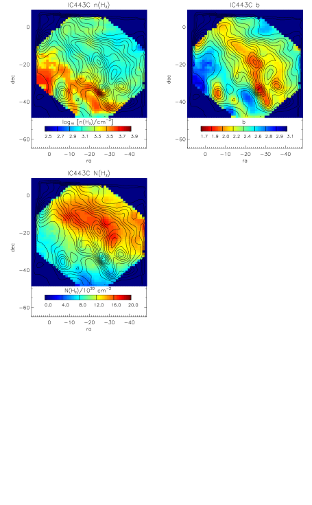
Figure 14: Spatial distributions of the best-fit-parameters for IC443C, including density $n$(H₂), power law index $b$ and column density of gas $N$(H₂) with 100 K $<T<$ 5000 K, calculated with IRS H₂ line emissions only. Regions are selected with S(5) intensity larger than 2 $\times$10${}^{-7}~{}$W m^-2sr^-1 so the signal-to-noise ratios for each H₂ lines are good enough to yield reliable fits. The contours of the brightest H₂ line S(5) are superposed.

The spatial distributions of the best-fit parameters – including the H₂ density, the power law index, $b$, the column density of warm hydrogen above 100 K, and the average OPR – are shown in Figure 14 – 19. The contours of the brightest H₂ line, S(5), are superposed. These parameter maps are obtained by fits to the H₂ IRS lines only, which have good signal-to-noise ratios. They are not intended to show the exact values of the parameters at each position but rather the spatial variations of the physical conditions in these regions. Here, we show only the averaged OPR over the column density of H₂ at every position, not OPR₀ and $n$(H)$\times$$\tau$ separately because these two parameters, like another pair of parameters, $n$(H₂) and $b$, are degenerate in the parameter space. Increasing either of them will raise the resultant OPR of the gas. Thus the confidence intervals are wide for these two parameters, especially for $n$(H)$\times$$\tau$. The much larger uncertainties in the line intensities at a single pixel, compared with the errors in the map-averaged intensities, make the derived OPR₀ and $n$(H)$\times$$\tau$ even more poorly constrained and unreliable. That is why we show the averaged OPR maps instead.

5 Discussion

5.1 The best-fit density

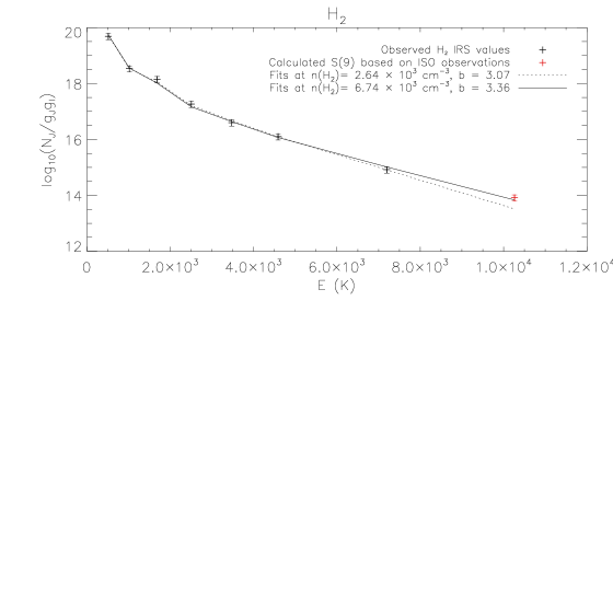
Figure 8: Similar to Figure 7. The dotted line represents fits to W28 H₂ rotational diagram computed with the IRS H₂ lines. The S(6) line flux is excluded which can not be measured reliably. The solid line shows fits calculated with both IRS H₂ lines and S(9)/S(3) ratio obtained by the $\it{ISO}$ SWS observation. The rightmost red cross shows S(9) evaluated with IRS S(3) intensity and the given SWS S(9)/S(3) ratio.

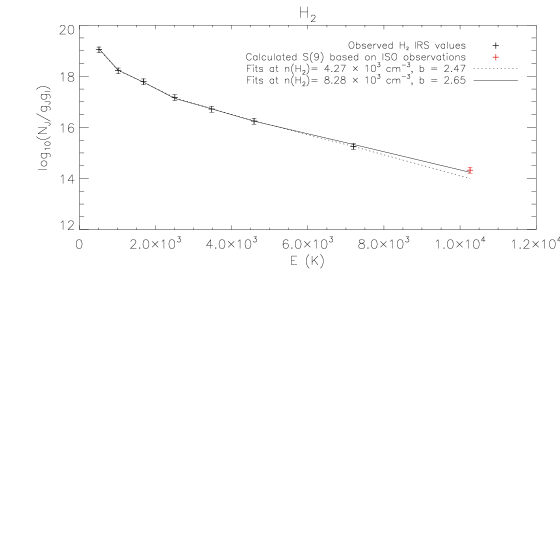
Figure 9: Same as Figure 8 but for W44. The H₂ S(6) line is not included as it cannot be measured reliably.

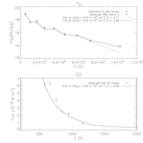
Figure 12: Same as Figure 7 but for HH54. The blue crosses in the lower panel represent observed CO fluxes at $J=14$–13, $J=15$–14, $J=16$–15, $J=17$–16, $J=18$–17 and $J=20$–19 respectively.

From Table 1 and Figures 7 – 12 we see that the H₂ pure rotational emissions detected by IRS of all six sources are consistent with excitation conditions in gas with $n$(H₂) $\sim$ 2 – 4 $\times 10^{3}$ cm^-3 and temperature index $b\sim$ 2.3 – 3.1. In the case of W28, W44 and 3C391, the intensities of H₂ S(9), however, suggest a denser region with $n$(H₂) 2 – 2.5 times larger, and including the IRAC band 2 (4.5 $\mu$m) brightness – contributed mainly by H₂ S(9) to S(12) – as well as the CO highly-excited rotational line fluxes, which are considered only in the case of IC443C and HH54, yields an even higher best-fit density with $n$(H₂) $\sim$ 1 – 4 $\times 10^{4}$ cm^-3. The latter density range is closer to estimates from previous studies of emissions from various species. Snell et al. (2005) found that a preshock density of 3$\times 10^{4}$ cm^-3 for either a slow J-type or C-type shock in IC443 clump C can account for the observed H₂O, CO, OH and H₂ 2 $\mu$m line intensities. For the other three SNRs – W28, W44 and 3C391 – the IRS regions coincide with the locations of the brightest 1720 MHz OH masers, the presence of which implies the existence of clumps of OH gas at moderate temperature 50 – 125 K and densities $n$(H₂) $\sim 10^{5}$ cm^-3 in C shocks (Lockett et al. 1999; Wardle & Yusef-Zadeh 2002). For HH54, the multi-species analysis done by Giannini et al. (2006) indicated that an 18 km s^-1 J-type shock with a continuous precursor and a density $n$(H₂) $\sim 10^{4}$ cm^-3 matches the H₂ vibrational and pure rotational lines, as well as the CO and H₂O emissions observed with ISO. Molinari et al. (2000) studied the HH 7–11 outflow emissions using ${\it ISO}$ and interpreted the H₂, CO and H₂O line emissions as emerging from a mixture of J- and C-type shocks propagating in gas of density $n$(H₂) $\sim 10^{4}$ cm^-3.

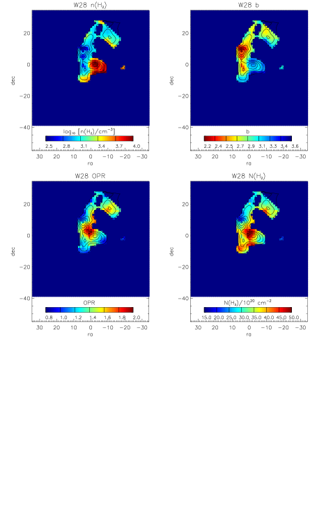
Figure 15: Same as Figure 14 but for W28. Parameter maps includes density $n$(H₂), power law index $b$, column density of gas $N$(H₂) with 100 K $<T<$ 5000 K and averaged OPR over the total column density. Regions are selected with S(5) intensity larger than 7.5 $\times$10${}^{-7}~{}$W m^-2sr^-1.

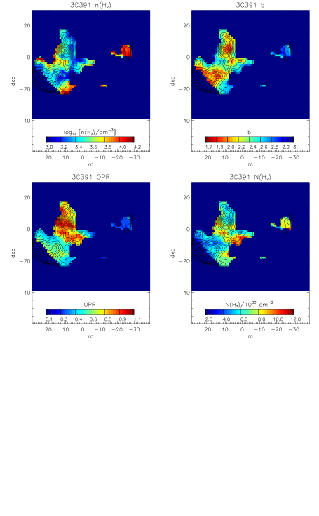
Figure 17: Similar as Figure 15 but for 3C391. Regions are selected with S(5) intensity larger than 7.9 $\times$10${}^{-7}~{}$W m^-2sr^-1.

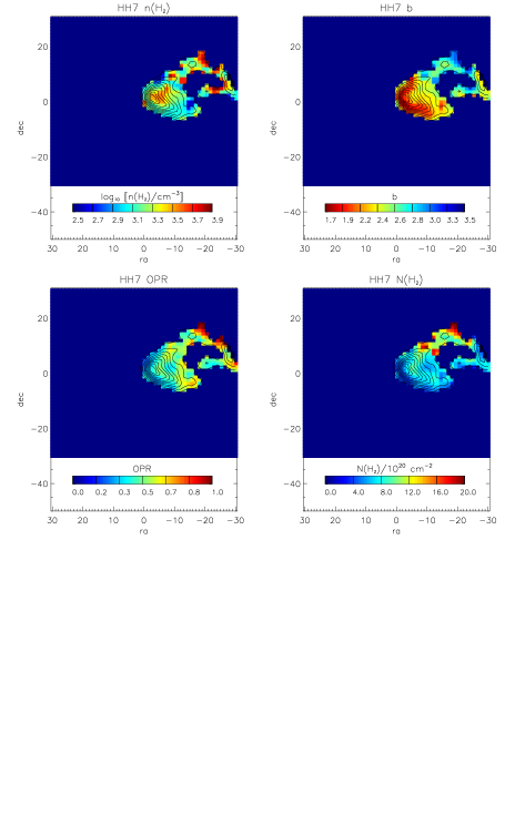
Figure 18: Same as Figure 15 but for HH7. Regions are selected with S(5) intensity larger than 2.0 $\times$10${}^{-7}~{}$W m^-2sr^-1.

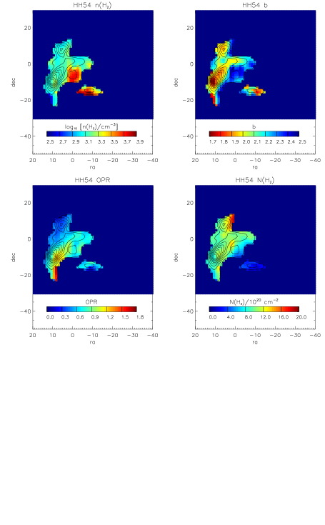
Figure 19: Similar as Figure 15 but for HH54. Regions are selected with S(5) intensity larger than 2.8$\times$10${}^{-7}~{}$W m^-2sr^-1.

The inconsistency among the best-fit densities estimated from different molecular species, obtained in the calculations described above, can be explained by the density fluctuations within the observed regions. The clouds may be composed of both moderate density gas with $n$(H₂) $\sim 10^{3}$ cm^-3 and dense cores with $n$(H₂) $\sim 10^{5}-10^{6}$ cm^-3. Indeed, the density maps derived from the IRS H₂ fluxes exhibit large variations within the small areas ($\sim~{}1^{{}^{\prime}}\times~{}1^{{}^{\prime}}$) mapped, as shown in Figures 14 – 19. The higher critical densities for the H₂ S(9) to S(12) transitions, the CO high-$J$ transitions as well as the H₂O lines, which we do not utilize here, make the line intensities more sensitive functions of density than those of the H₂ IRS transitions. Thus, denser regions contribute more to the total emission for these transitions of high critical density, leading to larger density estimates. However, another possibility also exists that the low-lying and high-lying lines may actually trace different components of the shock. Reach et al. (2005) proposed that H₂ S(9) can arise largely from the dissociative part of shock, while H₂ S(3) is attributed almost entirely to the non-dissociative shock. In reality, these two situations may both exist when part of the highly-excited CO and H₂ rotational lines come from warmer regions where the shock is partially dissociative and atomic hydrogen becomes an important collisional partner, an effect neglected in our model.

5.2 The best-fit temperature distribution index $b$

The best-fit power-law index $b$, which represents the gas temperature distribution along the line-of-sight, is in the range 2.3 – 3.1 according to our fits to the IRS H₂ emissions. If H₂ S(9) is also considered, $b$ is enhanced by $\sim$ 0.2, and a further increase of 0.3 – 0.6 is needed if the IRAC 4.5 $\mu$m band flux or CO lines are included. The above effects are probably caused by the degeneracy of the two parameters — $n$(H₂) and $b$ — as mentioned in Section 4; an increase in the best-fit density can be compensated for by a larger $b$ (i.e. by assuming the presence of less gas at high temperatures). The best-fit $b$ index for all six sources is smaller than predictions from a classical bow shock whose shape can be approximated as parabolic. According to Smith & Brand (1990), the effective shock surface area d$A$ with a perpendicular shock velocity $V_{s}$ is proportional to $V_{s}^{-4}dV_{s}$, which leads to a power-law index $b$ $\sim 3.8$ if the relationship between the column density and shock velocity given by equation B6 in N06 is adopted: $N$(H${}_{2})$ $\varpropto V_{s}^{-0.75}$ (NY08). A $b$ index smaller than 3.8 can be caused by a d$A$ which drops less steeply with velocity $V_{s}$ than does a parabolic shock. This would require that the curvature of the shock front be smaller than that of a parabola, or more probably, that there exists an admixture of shocks with different geometries whose shapes vary from planar to bow.

5.3 The covering factors within the IRS regions

The average column density of the shocked H₂ at $T>$ 100 K within the rectangular areas marked in Figures 1 – 6 varies from 2$\times$ $10^{20}~{}$cm^-2 to 4 $\times$ $10^{21}~{}$cm^-2, with the two Herbig-Haro objects the weakest sources of the total H₂ emissions. The length scale defined by $N$(H${}_{2})$/$n$(H${}_{2})$, which should be equal to the product of shock thickness and covering factor within the regions, is in the range of $10^{16}$ cm – $10^{18}$ cm. All sources except HH54 show $N$(H${}_{2})$/$n$(H${}_{2})$ above $10^{17}~{}$cm. The thickness of the shocks in these regions, obtained from expressions (B6) and (B7) from N06, should be less than $10^{17}~{}$cm. The analysis above implies that the covering factor for all six sources except HH54 is larger than unity; for W28 it is even as large as $\sim 6$. The high covering factors are not surprising because we are probably not observing these shocks face-on. The filamentary structures appearing in part of the maps of W28 and W44 imply the existence of individual shock fronts seen close to edge-on, as suggested by Reach et al. (2005). Actually, for most of the sources except HH7, the complicated morphology of the maps suggests a combination of shocks with different geometry and seen from different angles. For HH7, the well-defined bow-shaped structure probably represents a simplified situation. Smith et al. (2003) proposed that a bow shock moving at an angle of $\sim 30^{\circ}$ to the line-of-sight is consistent with the H₂ line profiles observed at different positions in HH7.

5.4 The OPR and the environmental difference between SNRs and Herbig-Haro objects

Though the physical sizes of the shock structures mapped by IRS for HH7 and HH54 are $\lesssim 0.1$ times smaller than those for SNRs, the best-fit density, index $b$ and H₂ column density do not significantly differ between these two classes of source. We noted, however, that the OPR for hot gas ($T>$ 1000 K) in HH7 and HH54 is lower than the LTE value $\sim 3$, while for all four SNRs the departure of the OPR from equilibrium is negligible at that high temperature. This phenomenon is also reflected in the H₂ rotational diagrams, where the zigzag pattern is more apparent for the two Herbig-Haro objects and is apparent even for the highest rotational levels. In our model, the equilibrium OPR of hot gas in the four SNRs requires a best-fit $n$(H)$\times$$\tau$ that is 0.6 – 3 orders of magnitude larger than that inferred for HH7 and HH54. This difference may be caused by a different atomic hydrogen density $n$(H) within gas around SNRs and Herbig-Haro objects. Fast SNR blast waves driving interstellar shocks with $V_{s}\geq 100$ km s^-1 can produce strong ultraviolet emissions that are responsible for the dissociation of H₂ in surrounding regions, while for Herbig-Haro objects the typical shock speeds are observed to be smaller (Herbig & Jones 1981;Cohen & Fuller 1985). Many high excitation fine structure lines which have been detected previously toward many SNRs are faint or absent toward Herbig-Haro objects. In addition to the UV field produced by nearby fast shocks, the X-ray emission from an SNR interior will also induce dissociation of pre-shock gas. These all imply that the molecular gas associated with Herbig-Haro objects probably subject to weaker photodissociation, which results in less H and a lower efficiency of para-to-ortho conversion. We note, however, that for measurements of near-infrared H₂ ro-vibrational transitions toward Herbig-Haro objects, the OPR values obtained are in most cases consistent with 3 (Smith, Davis & Lioure 1997). With energy levels lying above 6000 K, these vibrationally-excited lines originate mostly from the hottest part of the gas, which probably has a higher atomic fraction. These two factors – high temperature and high atomic H fraction – add up to a fast, efficient ortho-para conversion.

5.5 Maps of the parameters

The maps of best-fit parameters in Figures 14 – 19 were derived from the IRS H₂ fluxes only. So they may not represent the real average value at each pixel, but we expect that they carry useful information about spatial variations in the physical conditions in these regions. Maps of all six sources exhibit a spatial variation in $n$(H₂) larger than a factor 5, and a variation in $b$ larger than 1. The H₂ densities derived for a single pixel vary from $6\times 10^{2}$ cm^-2 to $10^{4}$ cm^-3, and the index $b$ ranges from 1.6 to 3.3.

After comparing the IRS H₂ spectroscopic maps with the parameter maps, we found that the maps of the temperature distribution index $b$ look most similar to the distributions of mid-lying H₂ emissions including S(3), S(4) and S(5). To show this similarity, we superpose the H₂ S(5) emission contours on these images. This fact implies that the emission in these mid-lying transitions is more strongly dependent on $b$ than on the density. In other words, these transitions, H₂ S(3) – S(5), trace mainly the hottest components of the gas. Since the gas temperature distribution at each position is determined largely by the shock velocity, these H₂ emissions may also serve as a good tracer of the local effective shock velocity. In HH7 for example, the S(3) – S(5) line intensities appear strongest near the head of the bow, where $V_{s}$ reaches its maximum. On the other hand, although the S(6) and S(7) emissions are also strongly affected by the gas temperature, they show more dependence upon $n$(H₂) compared to other lower-lying transitions. The critical densities for the excitation of S(6) and S(7) are higher than $10^{5}$ cm^-3 at the typical temperatures of relevance here. Thus, regions of enhanced density show up as clumpy features within the S(7) map for HH7. Finally, we note that the derived column density of H₂ at $T>$ 100 K is mostly determined by the intensities of the low-lying transitions, especially S(0). The S(0) emission arises mainly from lower temperature gas with $T<$ 500 K, which contributes most to the total $N$(H₂) for the power-law temperature distribution that we assume.

6 Summary

1. We have studied the physical conditions within shock-excited molecular gas associated with IC443C, W28, W44, 3C391, HH7 and HH54. We mainly used the H₂ S(0) to S(7) spectral line maps obtained by IRS on $Spitzer$ to constrain the best-fit parameters. IRS observations of HD emissions, IRAC band 2 (4.5 $\mu$m) intensity maps, and ISO measurements of the H₂ S(9)/S(3) ratio and the CO high-lying rotational lines (from $J$ = 14 – 13 to $J$ = 20 – 19) are also used when available to provide additional constraints.

2. A comparison between the IRS H₂ emission distribution and the IRAC maps for IC443C shows the IRAC band 2, 3 and 4 intensities are attributable almost entirely to H₂ pure rotational emissions. IRAC band 2 gives us access to the high-lying H₂ transitions S(9) to S(12) which are not available from IRS observations. For HH54, the similarity between the IRS H₂ and IRAC maps implies these IRAC band fluxes may come mostly from H₂ emissions as well. We assumed that the HH54 IRAC band 2 intensity is dominated by H₂ emissions and used it as an extra diagnostic in the model. For the other four sources the IRAC maps show either a strong continuum component from PAHs or dust or are heavily polluted by point sources.

3. We adopted a power-law temperature distribution for the shocked gas, with the column density of gas at temperature between $T$ and $T$ + $dT$ assumed to be proportional to $T^{-b}$, where $T$ ranges from 100 to 5000 K. The molecular line intensities are then modeled under the assumption of statistical equilibrium. We have checked the validity of this approximation for transitions of the three species H₂, HD and CO. Our calculations show the departure from statistical equilibrium for those rotational states involved in our calculation is negligible under all plausible density conditions in molecular shocks.

4. The best-fit densities determined from the IRS H₂ pure rotational lines S(0) to S(7) for all six sources are consistent with the excitation conditions in gas with $n$(H₂) $\sim$ 2 – 4 $\times 10^{3}$ cm^-3. The intensities of H₂ S(9), however, require an environment 2 – 2.5 times denser. In the case of IC443C and HH54, where the highly-excited CO rotational line intensities measured by ISO are reliable and IRAC 4.5 $\mu$m band fluxes were considered, we found the gas density determined by including all the data above is even larger: $n$(H₂) $\sim$ 1 – 4 $\times 10^{4}$ cm^-3. This inconsistency can be explained by density fluctuations within the observed regions. However, it is also possible that the low-lying and high-lying lines originate from different components of the shock.

5. For all six sources the best-fit power-law index $b$ derived from IRS H₂ S(0) to S(7) is in the range of 2.3 – 3.1. If H₂ S(9) is also considered, $b$ is enhanced by $\sim$ 0.2, and a further increase of 0.3 – 0.6 is needed if the CO lines or IRAC 4.5 $\mu$m band fluxes are also included. The best-fit $b$ index is smaller than predictions from a classical parabolic bow shock, which leads to a power-law index $\sim 3.8$. It can be understood if the average curvature of the shock front is smaller than that of a parabola — or if there exists an admixture of shocks whose shapes vary from planar to bow.

6. The OPR for hot gas ($T>$ 1000 K) in all four SNRs is fairly close to the LTE value of $3$, while for the two Herbig-Haro objects it is confirmed to be less than the LTE value even at $T>$ 1000 K. This difference may be caused by different preshock atomic hydrogen densities $n$(H) within gas around SNRs and Herbig-Haro objects. SNRs may be subject to heavier UV photodissociation and therefore produce more atomic hydrogen in the gas, which is the dominant collisional partner in the para-to-ortho conversion process in molecular shocks.

7. Unlike the OPR, the best-fit density, power-law index, $b$, and H₂ column density do not differ significantly between SNRs and Herbig-Haro objects. It should be noted that the acceptable ranges of the fitted parameters are actually large because they are degenerate in the parameter space ($n$(H₂) versus $b$ and OPR₀ versus $n$(H)$\times\tau$).

8. Given the observed IRS H₂ fluxes, we obtain upper limit on the CO abundance — $n$(CO)/$n$(H₂) — within the 80^′′ ISO/LWS beam of $1.5\times 10^{-3}$ and $5.5\times 10^{-4}$ for IC443C and HH54, respectively. Assuming that the CO emission distribution is similar to that of the IRAC bands (or the H₂ emission), we derive a rough estimate for the CO abundance of $n$(CO)/$n$(H₂) $\sim$ 3 – 5$\times 10^{-5}$ for IC443C and $n$(CO)/$n$(H₂) $\sim$ 2 – 4$\times 10^{-5}$ for HH54.

9. Parameter maps derived from the H₂ S(0) to S(7) lines for all six sources exhibit a spatial variation in $n$(H₂) larger than a factor 5 and a variation in $b$ larger than 1. The density, $n$(H₂), varies from $6\times 10^{2}$ to $10^{4}$ cm^-3, and the index $b$ ranges from 1.6 to 3.3.

10. Our maps of the best-fit parameters indicate that the mid-lying H₂ emissions — S(3) to S(5) — trace the hot component of the gas. On the other hand, the excitation of high-lying transitions, including S(6) and S(7), is more sensitive to the density of the gas. The spatial distribution of the H₂ column density with $T>$ 100 K is determined mainly by the lowest-lying transitions, particularly S(0).

Appendix A Evolution of level populations of H₂, HD, CO from non-equilibrium state

We present here a simple analysis of the relaxation timescale for the three species in shocks by solving the time-dependent population transfer equations

$$\sum_{J^{\prime}}\left(C_{J^{\prime}\rightarrow J}+A_{J^{\prime}\rightarrow J}\right)f_{J^{\prime}}-f_{J}\cdot\sum_{J^{\prime}}\left(C_{J\rightarrow J^{\prime}}+A_{J\rightarrow J^{\prime}}\right)={df_{J}\over dt},$$ (A1)

similar to equation (1) but with a time-dependent term.

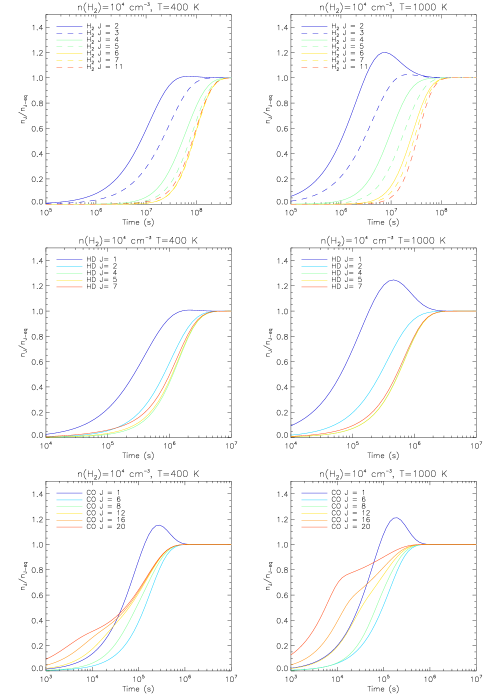
Figure 20: The evolution of level populations of H₂, HD and CO at density $n$(H₂) = 10⁴ cm^-3. $n_{J}$ denotes the level population density for level $J$ and $n_{J-eq}$ is the value at statistical equilibrium. The left panels are for $T$ = 400 K and right panels for $T$ = 1000 K, values which are consistent with typical temperatures of the warm and hot components (see text).

To solve the equations, all the molecules are assumed to be initially in the lowest quantum state. Here we treat ortho- and para- H₂ as distinct species due to the remarkably low efficiency of the para-to-ortho conversion processes, especially when compared with that of collisional and radiative transitions. Thus all para-H₂, HD and CO are put at $J=0$ and all ortho-H₂ are at $J=1$ at the beginning. The time evolution of the level populations for the three molecules at constant density $n$($H_{2}$) = 10⁴ cm^-3 and constant temperature $T$ = 400 K or $T$ = 1000 K (typical temperatures for the warm and hot components fitted by N06 & N07) are presented in Figure 20. The collisional partners were assumed to be molecular hydrogen and helium only. An average velocity gradient of 2 $\times$ 10^-10 cm s^-1/cm and a $n$(CO)/$n$(H₂) ratio of 5$\times 10^{-5}$ were adopted in calculating the CO optical depth. We note however, that these values do not affect greatly the evolution timescale.

From equation (A1), it is quite straightforward to see that the evolution depends on two processes — radiative decay and collisional excitation (and de-excitation). We can define a characteristic time $t_{1/2}$, at which the population of a certain level $J$ reaches one-half of that in statistical equilibrium. Apparently, at the low density limit where $n$(H₂) is smaller than the critical density for the transition between the lowest two levels, radiative processes dominate. Here, $t_{1/2}$ will approach 1/A_J→J-1. For the four species para-H₂, ortho-H₂, HD and CO, the critical densities at 400 K are of the order of 10 cm^-3, 10² cm^-3, 10² cm^-3 and 10³ cm^-3. By contrast, for extremely dense gas which is allowed to reach local thermal equilibrium (LTE), $t_{1/2}$ is determined by the inverse of the collisional excitation rate $\sim$ 1/C_J-1→J, where C_J-1→J is proportional to $n$(H₂). In most cases with density between the low and high limits, $t_{1/2}$ lies between 1/A_J→J-1 and 1/C_J-1→J. More generally, the time required to reach equilibrium, however, is determined by the rotational state that reaches equilibrium most slowly. We define a relaxation time as the time required for all level populations to achieve values within 5$\%$ of those attained in statistical equilbrium. For this definition, we include the first 18 levels of H₂, the first 8 levels of HD and the first 21 levels of CO. From figure 20 we see that at $n$(H₂) = 10⁴ cm^-3 and $T$ = 400 K, H₂, HD and CO have relaxation times of 2.1$\times$10⁸ s, 3$\times$10⁶ s and 4.6$\times$10⁵ s respectively. For a hotter gas component with $T=1000$ K, the relaxation times are reduced to 8$\times$10⁷ s, 1.6$\times$10⁶ s and 3.3$\times$10⁵ s. Assuming a shock velocity in the range of 10 – 20 km s^-1, and a typical H₂ column density of $\sim$ 3$\times$10²⁰ cm^-2 given by equation (B7) in N06 for planar shocks, the fluid will spend a flow time larger than 1.5$\times$ 10¹⁰ s passing through the whole shock affected region, much longer than the relaxation timescale defined above.

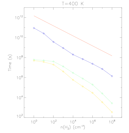
Figure 21: The dependence of the relaxation times upon H₂ density at 400 K. We define the relaxation time as the time needed for the level populations to attain values within 5$\%$ of the those obtained in statistical equilibrium. For H₂, we take the larger of the timescales calculated separately for para- and ortho-H₂. The blue, green and yellow squares represent values for H₂, HD and CO respectively. The red line marks the flow time; here we assumed $t_{flow}$ to be proportional to $n$(H₂)^-0.5 and equal to $\sim$ 1.5$\times$ 10¹⁰ s at $n$(H₂)= 10⁴ cm^-3.

If we assume a shocked H₂ column density proportional to $n$(H₂)^0.5 as given by equation (B7) in N06, the flow time $t_{flow}$ $\sim$ $N$(H₂)/($n$(H₂)$V_{S}$) will be proportional to $n$(H₂)^-0.5. Given a t_flow $\sim$ 1.5$\times$ 10¹⁰ s at $n$(H₂)= 10⁴ cm^-3, a comparison between relaxation times for H₂, HD, CO and the flow time at various densities with a typical shock velocity $\sim$ 20 km s^-1 is given in figure 21. It is apparent that, for modeling the molecular transitions accessible to infrared observatories including IRS, IRAC and ISO, the departure from statistical equilibrium for those levels involved is always negligible under all possible density conditions in molecular shocks.

Table 1: Observed fluxes and average line intensities

Species	IC443C	W28	W44	3C391	HH7	HH54
H2 S(0) 28.22 $\mu m$	0.14	0.37	0.079	0.13	0.093	0.058
H2 S(1) 17.04 $\mu m$	3.45	2.55	1.16	0.69	0.39	0.40
H2 S(2) 12.28 $\mu m$	4.42	3.45	1.39	0.96	1.65	1.79
H2 S(3) 9.67 $\mu m$	19.95	6.35	3.44	1.88	2.04	2.75
H2 S(4) 8.03 $\mu m$	8.05	2.06	2.47	1.60	2.16	2.95
H2 S(5) 6.91 $\mu m$	23.57	6.34	8.46	8.88	2.71	3.61
H2 S(6) 6.10 $\mu m$	5.08	…	…	…	1.10	1.80
H2 S(7) 5.51 $\mu m$	11.38	2.22	4.51	3.51	1.48	1.89
HD R(3) 28.50 $\mu m$	0.040	…	…	…	0.012	0.0093
HD R(4) 23.03 $\mu m$	0.017	…	…	…	0.0071	0.0075
H2 S(9)/S(3)	…	0.12	0.53	0.67	…	…
IRAC Band2(4.5 $\mu m$)	6.91	2.11	4.54	10.41	2.58	1.85
CO $J$=14-13 186.00 $\mu m$	…	…	…	9.0$\pm$2.2	6.6$\pm$2.1	6$\pm$1
CO $J$=15-14 173.63 $\mu m$	12.9$\pm$4.9	$<15$	…	28.8$\pm$2.3	8.5$\pm$2.8	6$\pm$1
CO $J$=16-15 162.81 $\mu m$	11.7$\pm$2.2	$<5$	$<5$	10.0$\pm$1.7	5.7$\pm$1.5	3.9$\pm$0.2
CO $J$=17-16 153.27 $\mu m$	6.7$\pm$0.9	…	…	10.3$\pm$2.8	8.4$\pm$3.0	2.2$\pm$0.3
CO $J$=18-17 144.78 $\mu m$	…	…	…	$<17$	…	2.1$\pm$0.3
CO $J$=19-18 137.20 $\mu m$	…	…	…	$<17$	…	$<1$
CO $J$=20-19 130.37 $\mu m$	…	…	…	$<17$	…	0.9$\pm$0.3

Table 2: Observed fluxes and average line intensities

Best-fit parameters	IC443C	W28	W44	3C391	HH7	HH54
Fits to IRS H2 lines only
$log_{10}$[$n$(H2)/cm-3]	3.36 (3.1 – 3.9)	3.42 (3.2 – 4.1)	3.63 (3.2 – 4.5)	3.62 (3.2 – 4.5)	3.39 (2.9 – 4.2)	3.30 (3.0 – 3.7)
Power law index, b	2.29 (1.9 – 2.7)	3.07 (2.7 – 3.7)	2.47 (2 – 3)	2.48 (2 – 3.1)	2.54 (2.2 – 3.1)	2.17 (1.8 – 2.6)
OPR0	3	1.23 ($\leq$2.7)	1.98 ($\leq$3)	0.255($\leq$1.8)	0.517 (0.2 – 1.1)	0.65 ($\leq$1.2)
$log_{10}$[$n$(H)$\times\tau/cm^{-3}$yr]	…	4.43 (…)	3.88 (…)	6.38 ($\geq$2.3)	3.25 (2.6 – 4.2)	3.01 ($\leq$3.7)
$log_{10}$[$N$(H2)/cm-2]	21.13	21.51	20.87	20.83	20.63	20.38
Fits to all reliable features
log10[$n$(H2)/cm-3]	4.1 (3.2 – 4.7)	3.83 (3.2 – 4.4)	3.92 (3.4 – 4.4)	3.91 (3.5 – 4.4)	3.41 (2.9 – 4.2)	4.51 (3.4 – 5.5)
Power law index, b	2.78 (2.2 – 3.2)	3.36 (2.8 – 3.9)	2.65 (2.2 – 3.1)	2.68 (2.2 – 3.1)	2.55 (2.2 – 3.1)	2.99 (2.4 – 3.3)
OPR0	3	1.44 ($\leq$3)	2.23 ($\leq$3)	0.493 ($\leq$2)	0.520 (0.2 – 1.1)	0.787 ($\leq$1.5)
log10[$n$(H)$\times\tau$/cm-3yr]	…	4.43 (…)	3.48 (…)	6.14 ($\geq$3.3)	3.25 (2.6 – 4.2)	2.82 ($\leq$3.6)
log10[$N$(H2)/cm-2]	21.32	21.61	20.95	20.92	20.63	20.69

Figure 13: $\chi^{2}$ contours in the $b$–n($H_{2}$) plane for all six sources. Dotted lines show fits calculated with IRS H₂ lines and solid lines for fits with all reliable features included. The best-fit $b$ and $n$(H₂) are marked by triangles and crosses for the two cases respectively. The inner contours confine the $68.3\%$ joint confidence interval and the outer contours confine the $95.4\%$ confidence interval. For HH7 the two sets of contours almost overlap each other.

Figure 16: Same as Figure 15 but for W44. Regions are selected with S(5) intensity larger than 8 $\times$10${}^{-7}~{}$W m^-2sr^-1.

References

- Balakrishnan et al. (2002) Balakrishnan, N., Yan, M. & Dalgarno, A. 2002, ApJ, 568, 443
- Bohigas et al. (1983) Bohigas, J., Ruiz, M. T., Carrasco, L., Salas, L., Herrera, M. A. 1983, RMxAA, 8, 155
- Cabrit et al. (1999) Cabrit, S., Bontemps, S., Lagage, P. O., et al. 1999, ESASP, 427, 449
- Chevalier et al. (1983) Chevalier, Roger A. 1999, ApJ, 511, 798
- Cohen & Fuller (1985) Cohen, M. & Fuller, G. A. 1985, ApJ, 296, 620
- DeNoyer (1978) Denoyer, L. K. 1978, MNRAS, 183, 187
- Fazio et al. (2004) Fazio, G. G., et al. 2004, ApJS, 154, 10
- Flower et al. (1998) Flower, D. R., Roueff, E., & Zeippen, C. J. 1998, J. Phys. B, 31, 1105
- (9) Flower, D. R. & Roueff, E. 1998a, J. Phys. B, 31, 2935
- (10) Flower, D. R. & Roueff, E. 1998b, J. Phys. B, 31, L955
- Flower & Roueff (1999) Flower, D. R. & Roueff, E. 1999, J. Phys. B, 32, 3399
- Flower (1999) Flower, D. R. 1999, J. Phys. B, 32, 1755
- Flower (2001) Flower, D. R. 2001, J. Phys. B, 34, 2731
- Forrey (1997) Forrey, R. C., Balakrishnan, N., Dalgarno, A., Lepp, S. 1997, ApJ, 489, 1000
- Graham & Hartigan (1988) Graham, J. A. & Hartigan, P. 1988, AJ, 95, 1197
- Giannini et al. (2006) Giannini, T., McCoey, C., Nisini, B., Cabrit, S., Caratti o Garatti, A., Calzoletti, L., Flower, D. R. 2006, A&A, 459, 821
- Gredel (1994) Gredel, R. 1994, A&A, 292, 580
- Gredel (1996) Gredel, R. 1996, A&A, 305, 582
- Harrus (1997) Harrus, I. M. 1997, ApJ, 488, 781
- Herbig & Jones (1981) Herbig, G. H. & Jones, B. F. 1981, AJ, 86, 1232
- Hughes & Hartigan (1992) Hughes, J. & Hartigan, P. 1992, AJ, 104, 680
- Liseau et al. (1996) Liseau, R., Ceccarelli, C., Larsson, B., et al. 1996, A&A, 315, 181
- Lockett et al. (1996) Lockett, P., Gauthier, E., Elitzur, M. 1999, ApJ, 511, 235
- Long et al. (1991) Long, K. S., Blair, W. P., Matsui, Y., White, R. L. 1991, ApJ, 373, 567
- Molinari et al. (2000) Molinari, S., Noriega-Crespo, A., Ceccarelli, C., et al. 2000, ApJ, 538, 698
- Neufeld & Kaufman (1993) Neufeld, D. A. & Kaufman M. J. 1993, ApJ, 418, 263
- Neufeld et al. (1998) Neufeld, D. A., Melnick, G. J., Harwit, M. 1998, ApJ, 506, 75
- N (06) Neufeld, D. A., Melnick, G. J., Sonnentrucker, P., et al. 2006, ApJ, 649, 816 (N06)
- N (07) Neufeld, D. A., Hollenbach, D. J., Kaufman, M. J., et al. 2007, ApJ, 664, 890 (N07)
- NY (08) Neufeld, D. A., & Yuan Y. 2008, ApJ, 678, 974 (NY08)
- N (09) Neufeld, D. A., Nisini, B., Giannini, T., et al. 2009, ApJ, 706, 170 (N09)
- Nisini et al. (1998) Nisini, B., Lorenzetti, D., Cohen, M., et al. 1996, A&A, 315, 321
- Reach & Rho (2001) Reach, W. T. & Rho, J. H. 2001, ApJ, 558, 943
- Reach et al. (2002) Reach, W. T., Rho, J. H., Jarrett, T. H., Lagage, P. 2002, ApJ, 564, 302
- Reach et al. (2005) Reach, W. T., Rho, J. H., Jarrett, T. H. 2005, ApJ, 618, 297
- Reach et al. (2006) Reach, W. T., Rho, J. H., Tappe, A., et al. 2006, AJ, 131, 147
- Rho et al. (1994) Rho, J. H., Petre, R., Schlegel, E. M., Hester, J. J. 1994, ApJ, 430, 757
- Rho & Peter (1996) Rho, J. H. & Peter, R. 1996, ApJ, 467, 698
- Rho & Peter (1998) Rho, J. H. & Peter, R. 1998, ApJ, 503, 167
- Richter (1995) Richter, M. J., Graham, J. R., Wright, G. S. 1995, ApJ, 454, 277
- Roueff & Flower (1999) Roueff, E. & Flower, D. R. 1999, MNRAS, 305, 353
- Roueff & Zeippen (1999) Roueff, E. & Zeippen, C. J. 1999, A&A, 343, 1005
- Sandell (1987) Sandell, G., Zealey, W. J., Williams, P. M., Taylor, K. N. R., Storey, J. V. 1987, A&A, 182, 237
- Schoier (2005) Schoier, F. L., van der Tak, F. F. S., van Dishoeck, E. F., Black, J. H. 2005, A&A, 432, 369
- Smith & Brand (1990) Smith, M. D. & Brand, P. W. J. L. 1990, MNRAS, 245, 108
- Smith, Brand & Moorhouse (1991) Smith, M. D., Brand, P. W. J. L. & Moorhouse, A. 1991, MNRAS, 248, 730
- Smith, Davis & Lioure (1997) mith, M. D., Davis, C. J., & Lioure, A. 1997, A&A, 327, 1206
- Smith et al. (2003) Smith, M. D., Khanzadyan, T., Davis, C. J. 2003, MNRAS, 339, 524
- Snell & Ewards (1981) Snell, R. L. & Edwards, S. 1981, ApJ, 251, 103
- Strom, Vbra & Strom, (1979) Strom, S. E., Vrba F. J. & Strom, K. M. Astron. J., 81, 314
- Timmermann (1998) Timmermann, R. 1998, ApJ, 498, 246
- Wardle & Yusef-Zadeh (2002) Wardle, M., Yusef-Zadeh, F. 2002, Sci, 296, 2350
- Weingartner & Draine (2001) Weingartner, J. C. & Draine, B. T. 2001, ApJ, 548, 296
- Wernli et al. (2006) Wernli, M., Valiron, P., Faure, A., Wiesenfeld, L., Jankowski, P., Szalewicz, K. 2006, A&A, 446, 367
- Wilgenbus et al. (2000) Wilgenbus, D., Cabrit, S., Pineau des Forets, G., Flower, D. R. 2000, A&A, 356, 1010