Function Photonic Crystals

Abstract

In the paper, we present a new kind of function photonic crystals, which refractive index is a function of space position. Unlike conventional PCs, which structure grow from two materials, A and B, with different dielectric constants $\varepsilon_{A}$ and $\varepsilon_{B}$. Based on Fermat principle, we give the motion equations of light in one-dimensional, two-dimensional and three-dimensional function photonic crystals. For one-dimensional function photonic crystals, we investigate the dispersion relation, band gap structure and transmissivity, and compare them with conventional photonic crystals. By choosing various refractive index distribution function $n(z)$, we can obtain more wider or more narrower band gap structure than conventional photonic crystals.
PACS: 42.70.Qs, 78.20.Ci, 41.20.Jb
Keywords: Photonic crystals; Refractive index; Electromagnetic wave propagation

1. Introduction

Photonic crystals (PCs), proposed by Yablonovitch and John, represent a novel class of optical materials which allow to control the flow of electromagnetic radiation or to modify light-matter interaction [1, 2]. These artificial structures are characterized by one, two or three-dimensional arrangements of dielectric material which lead to the formation of an energy band structure for electromagnetic waves propagating in them. One of the most attractive features of photonic crystals is associated with the fact that PCs may exhibit frequency ranges over which ordinary linear propagation is forbidden, irrespective of direction. These photonic band gaps (PBGs) lend themselves to numerous diversified applications (in linear, nonlinear and quantum optics). For instance, PBG structures with line defects can be used for guiding light. Similarly, as it has been predicted and confirmed experimentally, photonic crystals allow to modify spontaneous emission rate due to the modification of density of quantum states. In particular, it is well known that the density of states grows at the edge of the photonic band gap of the PCs. This allows us to predict a higher optical gain, but on the other hand a higher level of noise in light generated in PC-lasers operated at a frequency near the band gap.

Photonic crystals are usually viewed as an optical analog of semiconductors that modify the properties of light similarly to a microscopic atomic lattice that creates a semiconductor band gap for electrons [3]. It is therefore believed that by replacing relatively slow electrons with photons as the carriers of information, the speed and bandwidth of advanced communication systems will be dramatically increased, thus revolutionizing the telecommunication industry. To employ the high-technology potential of photonic crystals, it is crucially important to achieve a dynamical tunability of their band gap [4]. This idea can be realized by changing the light intensity in the so-called nonlinear photonic crystals, having a periodic modulation of the nonlinear refractive index [5]. Exploration of nonlinear properties of photonic band-gap (PBG) materials could be exploited new applications of photonic crystals to devise all-optical signal processing and switching, which indicates an effective way to generate tunable band-gap structures by operating entirely with light.

During the past few years, there has been a great deal of interest in studying propagation of waves inside periodic structures. These systems are composites made of inhomogeneous distribution of some material periodically embedded in other with different physical properties. Phononic crystals (PCs)[6, 7] are one of the examples of these systems. PCs are the extension of the so-called Photonic crystals[8] when elastic and acoustic waves propagate in periodic structures made of materials with different elastic properties. When one of these elastic materials is a fluid medium, then PCs are called Sonic Crystals (SC)[9, 10]. For these artificial materials, both theoretical and experimental results have shown several interesting physical properties [11]. In the homogenization limit [12], it is possible to design acoustic metamaterials that can be used to build refractive devices [13]. In the range of wavelengths similar to the periodicity of the PCs, multiple scattering process inside the PC leads to the phenomenon of so called Band Gaps (BG),which are required for filtering sound [10], trapping sound in defects [14, 15] and for acoustic wave guiding [16].

In the present work we present a new kind of function photonic crystals, which refractive index is a function of the space position. Unlike conventional PCs, which grow from two materials, A and B, with different dielectric constants $\varepsilon_{A}$ and $\varepsilon_{B}$: a periodic layered medium $...A/B/A/B...$ in case of one-dimensional photonic crystals and periodic arrays of cylinders and spheres of the material A embedded in a dielectric matrix B, in case of two-dimensional and three-dimensional photonic crystals, respectively. Function PCs may extend the concept of PCs, leading likely to some new applications. To exemplify the idea of function PCs, we present theoretical calculations of the function photonic crystals band structures and transmissivity. Our results indicate that the function photonic crystals behaves more width or more narrow band gap structure than the conventional photonic crystals.

2. The light motion equation in function photonic crystals

For the function photonic crystals, the crystals refractive index is a periodic function of the space position, which can be written as $n(z)$, $n(x,z)$ $n(x,y,z)$ corresponding to one-dimensional, two-dimensional and three-dimensional function photonic crystals. In the following, we shall deduce the light motion equations for the one-dimensional, two-dimensional and three-dimensional function photonic crystals. Firstly, we give the light motion equation in one-dimensional function photonic crystals, and two-dimensional motion space, i.e., the refractive index is $n=n(z)$, meanwhile motion path is on $xz$ plane. The incident light wave strikes plane interface $A$ point, the curves $AB$ and $BC$ are the path of incident and reflected light respectively, and they are shown in FIG. 1.

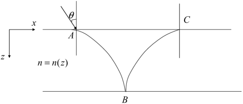
Figure 1: The motion path of light in one-dimensional function photonic crystals and two-dimensional motion space

The light motion equation can be obtained by Fermat principle, and it is

$$\delta\int^{B}_{A}n(z)ds=0.$$ (1)

In the two-dimensional transmission space, the line element $ds$ is

$$ds=\sqrt{(dx)^{2}+(dz)^{2}}=\sqrt{1+\dot{z}^{2}}dx,$$ (2)

where $\dot{z}=\frac{dz}{dx}$, then Eq. (1) becomes

$$\delta\int^{B}_{A}n(z)\sqrt{1+(\dot{z})^{2}}dx=0.$$ (3)

The Eq. (3) change into

$$\int^{B}_{A}(\frac{\partial(n(z)\sqrt{1+\dot{z}^{2}})}{\partial z}\delta z+\frac{\partial(n(z)\sqrt{1+\dot{z}^{2}})}{\partial\dot{z}}\delta\dot{z})dx=0,$$ (4)

i.e.,

$$\int^{B}_{A}\frac{dn(z)}{dz}\sqrt{1+\dot{z}^{2}}\delta zdx+\int^{B}_{A}n(z)\dot{z}(1+\dot{z}^{2})^{-\frac{1}{2}}d\delta z$$ (5)

$$= \int^{B}_{A}\frac{dn(z)}{dz}\sqrt{1+\dot{z}^{2}}\delta zdx+n(z)\dot{z}(1+\dot{z}^{2})^{-\frac{1}{2}}\delta z|^{B}_{A}-\int^{B}_{A}d(n(z)\dot{z}(1+\dot{z}^{2})^{-\frac{1}{2}})\delta z$$

$$= 0.$$

The two end points $A$ and $B$, their variation is zero, i.e., $\delta z(A)=\delta z(B)=0$, and the Eq. (5) is

$$\int^{B}_{A}(\frac{dn(z)}{dz}\sqrt{1+\dot{z}^{2}}-\frac{dn(z)}{dz}\dot{z}^{2}(1+\dot{z}^{2})^{-\frac{1}{2}}-n(z)\frac{\ddot{z}\sqrt{1+\dot{z}^{2}}-\dot{z}^{2}\ddot{z}(1+\dot{z}^{2})^{-\frac{1}{2}}}{1+\dot{z}^{2}})\delta zdx=0.$$ (6)

For arbitrary variation $\delta z$, there is

$$\frac{dn(z)}{dz}\sqrt{1+\dot{z}^{2}}-\frac{dn(z)}{dz}\dot{z}^{2}(1+\dot{z}^{2})^{-\frac{1}{2}}-n(z)\frac{\ddot{z}\sqrt{1+\dot{z}^{2}}-\dot{z}^{2}\ddot{z}(1+\dot{z}^{2})^{-\frac{1}{2}}}{1+\dot{z}^{2}}=0,$$ (7)

simplify Eq. (7), we have

$$\frac{dn(z)}{dz}-n(z)\frac{\ddot{z}}{1+\dot{z}^{2}}=0.$$ (8)

The Eq. (8) is light motion equation in one-dimensional function photonic crystals and two-dimensional motion space. Similarly, we can attain light motion equation in one-dimensional function photonic crystals and three-dimensional motion space. It is

$$\frac{dn(z)}{dz}\dot{y}(1+\dot{y}^{2}+\dot{z}^{2})-n(z)(\dot{y}\ddot{z}-\dot{z}\ddot{y})=0.$$ (9)

For the two-dimensional function photonic crystals, light in two-dimensional motion space, the light motion equation is

$$\frac{\partial n(x,z)}{\partial z}-n(x,z)\frac{\ddot{z}}{1+\dot{z}^{2}}-\frac{\partial n(x,z)}{\partial x}\dot{z}=0,$$ (10)

and the light in three-dimensional motion space, the motion equation is

$$\frac{\partial n(x,z)}{\partial z}\dot{y}(1+\dot{y}^{2}+\dot{z}^{2})-n(x,z)(\dot{y}\ddot{z}-\dot{z}\ddot{y})=0.$$ (11)

For the three-dimensional function photonic crystals, light in two-dimensional motion space, the light motion equation is

$$\frac{\partial n(x,y_{0},z)}{\partial z}-\frac{\partial n(x,y_{0},z)}{\partial x}\dot{z}-n(x,y_{0},z)\frac{\ddot{z}}{1+\dot{z}^{2}}=0,$$ (12)

where $y_{0}$ is constant, and the light transmits in three-dimensional motion space, the light motion equation is

$$(1+\dot{y}^{2}+\dot{z}^{2})(\frac{\partial n(x,y,z)}{\partial y}\dot{z}-\frac{\partial n(x,y,z)}{\partial z}\dot{y})-n(x,y,z)(\ddot{y}\dot{z}-\ddot{z}\dot{y})=0.$$ (13)

3. The transfer matrix of one-dimensional function photonic crystals

In this section, we should calculate the transfer matrix of one-dimensional function photonic crystals and two-dimensional motion space. In fact, it is the reflection and refraction of light at a plane surface of two media with different dielectric properties. The dynamic properties of the electric field and magnetic field are contained in the boundary conditions: normal components of $D$ and $B$ are continuous; tangential components of $E$ and $H$ are continuous. We consider the electric field perpendicular to the plane of incidence, and the coordinate system and symbols as shown in FIG. 2.

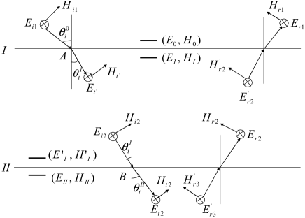
Figure 2: The light transmission figure in arbitrary middle medium

On the two sides of interface I, the tangential components of electric field $E$ and magnetic field $H$ are continuous, there are

$$\left\{\begin{array}[]{ll}E_{0}=E_{I}=E_{t1}+E^{\prime}_{r2}\\ H_{0}=H_{I}=H_{t1}\cos\theta_{t}^{I}-H^{\prime}_{r2}\cos\theta_{t}^{I},\end{array}\right.$$ (16)

On the two sides of interface II, the tangential components of electric field $E$ and magnetic field $H$ are continuous, and give

$$\left\{\begin{array}[]{ll}E_{II}=E^{\prime}_{I}=E_{i2}+E_{r2}\\ H_{II}=H^{\prime}_{I}=H_{i2}\cos\theta_{i}^{I}-H_{r2}\cos\theta_{i}^{I},\end{array}\right.$$ (19)

the electric field ${E_{t1}}$ is

$$E_{t1}=E_{t10}{e^{i(k_{x}x_{A}+k_{z}z)}|_{z=0}}=E_{t10}e^{i\frac{\omega}{c}n(0)\sin\theta_{t}^{I}x_{A}},$$ (20)

and the electric field ${E_{i2}}$ is

$$E_{i2}=E_{t10}{e^{i(k^{\prime}_{x}x_{B}+k^{\prime}_{z}z)}|_{z=b}}=E_{t10}e^{i\frac{\omega}{c}n(b)(\sin\theta_{i}^{I}x_{B}+\cos\theta_{i}^{I}b)}.$$ (21)

Where $x_{A}$ and $x_{B}$ are $x$ component coordinates corresponding to $A$ and $B$ points.
Now, we calculate the incident angle $\theta_{i}^{I}$. From Eq. (8), it is straightforward to derive

$$\frac{dn(z)}{n(z)}=\frac{\dot{z}d\dot{z}}{1+\dot{z}^{2}},$$ (22)

then integrate the two sides of Eq. (18)

$$\int^{n(b)}_{n(0)}\frac{dn(z)}{n(z)}=\int^{k_{b}}_{k_{0}}\frac{\dot{z}d\dot{z}}{1+\dot{z}^{2}},$$ (23)

to get

$$(\frac{n(b)}{n(0)})^{2}=\frac{1+k_{b}^{2}}{1+k_{0}^{2}},$$ (24)

where

$$k_{b}={\frac{dz}{dx}}|_{z=b}=\cot\theta_{i}^{I},$$ (25)

$$k_{0}={\frac{dz}{dx}}|_{z=0}=\cot\theta_{t}^{I},$$ (26)

and

$$\theta_{t}^{I}=\arcsin(\frac{n_{0}}{n(0)}\sin\theta_{i}^{0}),$$ (27)

where $n_{0}$ is air refractive index, and $n(0)=n(z)|_{z=0}$.
By substituting Eqs. (21), (22) and (23) into (20), we attain

$$\frac{1+\cot^{2}\theta_{i}^{I}}{1+\cot^{2}\theta_{t}^{I}}=\frac{n^{2}(b)}{n^{2}(0)}.$$ (28)

From Eq. (24), we can find when $n(0)=n(b)$, there is

$$\theta_{t}^{I}=\theta_{i}^{I}.$$ (29)

Integrate the two sides of Eq. (18), we can obtain the coordinate component $x_{B}$

$$\int^{n(z)}_{n(0)}\frac{dn(z)}{n(z)}=\int^{k_{z}}_{k_{0}}\frac{\dot{z}d\dot{z}}{1+\dot{z}^{2}},$$ (30)

to get

$$(\frac{n(z)}{n(0)})^{2}=\frac{1+k_{z}^{2}}{1+k_{0}^{2}},$$ (31)

since $k_{z}>0$, there is

$$k_{z}=\frac{dz}{dx}=\sqrt{(1+k_{0}^{2})(\frac{n(z)}{n(0)})^{2}-1},$$ (32)

i.e.,

$$dx=\frac{dz}{\sqrt{(1+k_{0}^{2})(\frac{n(z)}{n(0)})^{2}-1}}.$$ (33)

Obviously, $n(z)>n(0)\sin\theta^{I}_{t}$. The coordinate $x_{B}$ can be obtained as

$$x_{B}=x_{A}+\int^{b}_{0}\frac{dz}{\sqrt{(1+k_{0}^{2})(\frac{n(z)}{n(0)})^{2}-1}}.$$ (34)

By substituting Eq. (30) into (17), there is

$$E_{i2}=E_{t10}\exp[{i\frac{\omega}{c}n(b)(\sin\theta_{i}^{I}\int^{b}_{0}\frac{dz}{\sqrt{(1+k_{0}^{2})(\frac{n(z)}{n(0)})^{2}-1}}+\sin\theta_{i}^{I}x_{A}+\cos\theta_{i}^{I}b)}],$$ (35)

With substituting Eq. (16) into (31), there is

$$E_{i2} = E_{t1}e^{i{\delta}_{b}},$$ (36)

where

$$\delta_{b}=\frac{\omega}{c}n(b)(\cos\theta_{i}^{I}b+\sin\theta_{i}^{I}\int^{b}_{0}\frac{dz}{\sqrt{(1+k_{0}^{2})(\frac{n(z)}{n(0)})^{2}-1}}),$$ (37)

and similarly

$$E^{\prime}_{r2}=E_{r2}e^{i\delta_{b}}.$$ (38)

Substituting Eqs. (32) and (34) into (14) and (15), and using $H=\sqrt{\frac{\varepsilon_{0}}{\mu_{0}}}nE$, there are

$$\left\{\begin{array}[]{ll}E_{I}=E_{t1}+E_{r2}e^{i\delta_{b}}\\ H_{I}=\sqrt{\frac{\varepsilon_{0}}{\mu_{0}}}n(0)E_{t1}\cos\theta_{t}^{I}-\sqrt{\frac{\varepsilon_{0}}{\mu_{0}}}n(0)E_{r2}\cos\theta_{t}^{I}e^{i\delta_{b}},\end{array}\right.$$ (41)

and

$$\left\{\begin{array}[]{ll}E_{II}=E_{t1}e^{i\delta_{b}}+E_{r2}\\ H_{II}=\sqrt{\frac{\varepsilon_{0}}{\mu_{0}}}n(b)E_{t1}e^{i\delta_{b}}\cos\theta_{i}^{I}-\sqrt{\frac{\varepsilon_{0}}{\mu_{0}}}n(b)E_{r2}\cos\theta_{i}^{I}.\end{array}\right.$$ (44)

From Eq. (35) and (36), we can obtain

$$\left\{\begin{array}[]{ll}E_{I}=\frac{1}{\sqrt{\frac{\varepsilon_{0}}{\mu_{0}}}n(b)\cos\theta_{i}^{I}}(\sqrt{\frac{\varepsilon_{0}}{\mu_{0}}}n(b)\cos\theta_{i}^{I}\cos\delta_{b}E_{II}-i\sin\delta_{b}H_{II})\\ H_{I}=\frac{n(0)\cos\theta^{I}_{t1}}{n(b)\cos\theta^{I}_{i2}}(-i\sqrt{\frac{\varepsilon_{0}}{\mu_{0}}}n(b)\cos\theta_{i}^{I}\sin\delta_{b}E_{II}+\cos\delta_{b}H_{II}),\end{array}\right.$$ (47)

or

$$\left(\begin{array}[]{c}E_{I}\\ H_{I}\\ \end{array}\right)=\left(\begin{array}[]{cc}\cos\delta_{b}&-\frac{i\sin\delta_{b}}{\sqrt{\frac{\varepsilon_{0}}{\mu_{0}}}n(b)\cos\theta_{i}^{I}}\\ -i\sqrt{\frac{\varepsilon_{0}}{\mu_{0}}}n(0)\cos\theta_{t}^{I}\sin\delta_{b}&\frac{n(0)\cos\theta_{t}^{I}}{n(b)\cos\theta_{i}^{I}}\cos\delta_{b}\\ \end{array}\right)\left(\begin{array}[]{c}E_{II}\\ H_{II}\\ \end{array}\right),$$ (54)

define $M$ matrix

$$\left(\begin{array}[]{c}E_{I}\\ H_{I}\\ \end{array}\right)=M\left(\begin{array}[]{c}E_{II}\\ H_{II}\\ \end{array}\right)$$ (59)

where

$$M=\left(\begin{array}[]{cc}\cos\delta_{b}&-\frac{i}{\sqrt{\frac{\varepsilon_{0}}{\mu_{0}}}n(b)\cos\theta_{i}^{I}}\sin\delta_{b}\\ -i\sqrt{\frac{\varepsilon_{0}}{\mu_{0}}}n(0)\cos\theta_{t}^{I}\sin\delta_{b}&\frac{n(0)\cos\theta_{t}^{I}}{n(b)\cos\theta_{i}^{I}}\cos\delta_{b}.\\ \end{array}\right).$$ (62)

The Eq. (40) is the transfer matrix $M$ of the half period. When $n(0)=n(b)$, there is

$$\theta_{t}^{I}=\theta_{i}^{I},$$ (63)

and the $M$ matrix becomes

$$M=\left(\begin{array}[]{cc}\cos\delta_{b}&-\frac{i}{\eta_{b}}\sin\delta_{b}\\ -i\eta_{b}\sin\delta_{b}&\cos\delta_{b}\\ \end{array}\right),$$ (66)

where $\eta_{b}=\sqrt{\frac{\varepsilon_{0}}{\mu_{0}}}n(0)\cos\theta_{i}^{I}$. In the following, we should study the one-dimensional function Photonic crystals at $n(0)=n(b)$.

4. The structure of one-dimensional function photonic crystals

In section 3, we attain the $M$ matrix of the half period. We know that the conventional photonic crystals is constituted by two different refractive index medium, and the refractive indexes are not continuous on the interface of the two medium. We could devise the one-dimensional function photonic crystals structure as follows: in the first half period, the medium refractive index is $n_{1}(z)$, and in the second half period, the medium refractive index is $n_{2}(z)$, corresponding thickness $b$ and $a$, respectively. Their refractive indexes satisfy condition $n_{1}(b)\neq n_{2}(0)$, as shown in FIG. 3. We should discuss two kinds of incidence cases:
(1) The light vertical incidence

For the vertical incidence, the initial incidence angle $\theta_{i}^{0}=0$ and refraction angle $\theta_{t}^{I}=0$. From Eq. (41), there is

$$\theta_{i}^{I}=0,$$ (67)

then

$$\theta_{t}^{II}=0,\hskip 21.68121pt\theta_{i}^{II}=0,\hskip 21.68121pt\theta_{t}^{III}=0,\hskip 10.84006pt\cdots$$ (68)

i.e., all incidence angles and refraction angles are zero, and the $M$ matrix is

$$M=\left(\begin{array}[]{cc}\cos\delta_{b}&-\frac{i}{\eta_{b}}\sin\delta_{b}\\ -i\eta_{b}\sin\delta_{b}&\cos\delta_{b}\\ \end{array}\right).$$ (71)

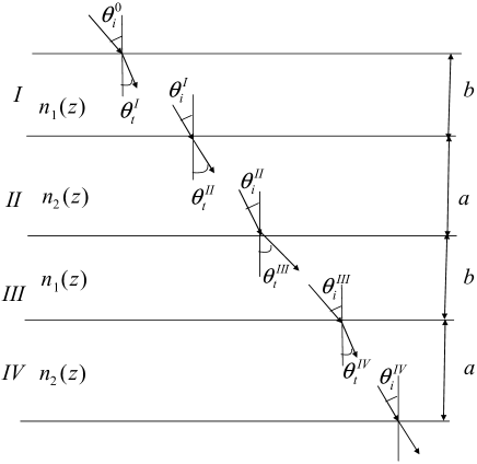
Figure 3: The two periods transmission figure of light in function photonic crystals

Where $\delta_{b}=\frac{\omega}{c}n(b)b$ and $\eta_{b}=\sqrt{\frac{\epsilon_{0}}{\mu_{0}}}n(b)$. In the case, the function photonic crystals becomes conventional common photonic crystals, which its refractive indexes $n_{a}$ and $n_{b}$ are constants.
(2) The light non-vertical incidence

For light non-vertical incidence, the initial incidence angle $\theta^{0}_{i}\neq 0$ in the first half period $I$.
By refraction law, there is

$$\sin\theta^{I}_{t}=\frac{n_{0}}{n_{1}(0)}\sin\theta^{0}_{i},$$ (72)

where $n_{0}$ is air refractive indexes, and $n_{1}(0)=n_{1}(z)|_{z=0}$.
when $n_{1}(0)=n_{1}(b)$, $\theta^{I}_{i}=\theta^{I}_{t}$, we obtain the $M_{b}$ matrix in the first half period $I$ as

$$M^{I}_{b}=\left(\begin{array}[]{cc}\cos\delta^{I}_{b}&-\frac{i}{\eta^{I}_{b}}\sin\delta^{I}_{b}\\ -i\eta^{I}_{b}\sin\delta^{I}_{b}&\cos\delta^{I}_{b}\\ \end{array}\right)$$ (75)

where

$$\eta^{I}_{b}=\sqrt{\frac{\varepsilon_{0}}{\mu_{0}}}n_{1}(0)\cos\theta^{I}_{t}$$ (76)

and

$$\delta^{I}_{b}=\frac{\omega}{c}n_{1}(0)[\cos\theta^{I}_{t}\cdot b+\sin\theta^{I}_{t}\int^{b}_{0}\frac{dz}{\sqrt{(1+k_{0}^{2})(\frac{n_{1}(z)}{n_{1}(0)})^{2}-1}}].$$ (77)

Where $k_{0}=\cot\theta_{t}^{I}$.
In the second half period $II$, by refraction law, there is

$$\sin\theta^{II}_{t}=\frac{n_{1}(b)}{n_{2}(0)}\sin\theta^{I}_{i},$$ (78)

when $n_{2}(0)=n_{2}(a)$, we have

$$\theta^{II}_{i}=\theta^{II}_{t},$$ (79)

The $M_{a}$ matrix in the second half period $II$ is obtained

$$M^{I}_{a}=\left(\begin{array}[]{cc}\cos\delta^{II}_{a}&-\frac{i}{\eta^{II}_{a}}\sin\delta^{II}_{a}\\ -i\eta^{II}_{a}\sin\delta^{II}_{a}&\cos\delta^{II}_{a}\\ \end{array}\right),$$ (82)

where

$$\eta^{II}_{a}=\sqrt{\frac{\varepsilon_{0}}{\mu_{0}}}n_{2}(0)\cos\theta^{II}_{t},$$ (83)

and

$$\delta^{II}_{a}=\frac{\omega}{c}n_{2}(0)[\cos\theta^{II}_{t}\cdot a+\sin\theta^{II}_{t}\int^{a}_{0}\frac{dz}{\sqrt{(1+k_{I}^{2})(\frac{n_{2}(z)}{n_{2}(0)})^{2}-1}}],$$ (84)

where $k_{I}=\cot\theta_{t}$. From Eqs. (46) and (50), we have

$$\sin\theta^{II}_{t}=\frac{n_{0}}{n_{2}(0)}\sin\theta^{0}_{i},$$ (85)

and

$$\cos\theta^{II}_{t}=\sqrt{1-\frac{n_{0}^{2}}{(n_{2}(0))^{2}}\sin^{2}\theta^{0}_{i}}.$$ (86)

Then the $M$ matrix in the first period is expressed as

$$M^{I}=M^{I}_{b}\cdot M^{I}_{a}$$ (87)

In the next, we should calculate the $M$ matrix in the second period.
By refraction law, there is

$$\sin\theta^{III}_{t}=\frac{n_{2}(b)}{n_{1}(0)}\sin\theta^{II}_{i}=\frac{n_{0}}{n_{1}(0)}\sin\theta^{0}_{i}=\sin\theta^{I}_{t}$$ (88)

when $n_{1}(0)=n_{1}(b)$, we have

$$\theta^{III}_{i}=\theta^{III}_{t}=\theta^{I}_{t},$$ (89)

We can obtain the $M_{b}$ matrix in the second period

$$M^{II}_{b}=\left(\begin{array}[]{cc}\cos\delta^{III}_{b}&-\frac{i}{\eta^{III}_{b}}\sin\delta^{III}_{b}\\ -i\eta^{III}_{b}\sin\delta^{III}_{b}&\cos\delta^{III}_{b}\\ \end{array}\right)$$ (92)

where

$$\eta^{III}_{b}=\sqrt{\frac{\varepsilon_{0}}{\mu_{0}}}n_{1}(0)\cos\theta^{III}_{t}=\eta^{I}_{b},$$ (93)

$$\delta^{III}_{b}=\frac{\omega}{c}n_{1}(0)[\cos\theta^{III}_{t}\cdot b+\sin\theta^{III}_{t}\int^{b}_{0}\frac{dz}{\sqrt{(1+k_{II}^{2})(\frac{n_{1}(z)}{n_{1}(0)})^{2}-1}}]=\delta^{1}_{b}.$$ (94)

From Eqs. (60)-(62), we find

$$M_{b}^{II}=M_{b}^{I}.$$ (95)

Now, we calculate the $M_{a}$ matrix in the second period.
By refraction law, there is

$$\sin\theta^{IV}_{t}=\frac{n_{1}(b)}{n_{2}(0)}\sin\theta^{III}_{i}=\frac{n_{0}}{n_{2}(0)}\sin\theta^{0}_{i}=\sin\theta^{II}_{t},$$ (96)

when $n_{2}(0)=n_{2}(a)$, we have

$$\theta^{IV}_{i}=\theta^{IV}_{t}=\theta^{II}_{t}$$ (97)

We can obtain the $M_{a}$ matrix in the second half period $IV$ of the second period

$$M^{II}_{a}=\left(\begin{array}[]{cc}\cos\delta^{IV}_{a}&-\frac{i}{\eta^{IV}_{a}}\sin\delta^{IV}_{a}\\ -i\eta^{IV}_{a}\sin\delta^{IV}_{b}&\cos\delta^{IV}_{b}\\ \end{array}\right),$$ (100)

where

$$\eta^{IV}_{a}=\sqrt{\frac{\varepsilon_{0}}{\mu_{0}}}n_{2}(0)\cos\theta^{IV}_{t}=\eta^{II}_{a},$$ (101)

and

$$\delta^{IV}_{a}=\frac{\omega}{c}n_{2}(0)[\cos\theta^{IV}_{t}a+\sin\theta^{IV}_{t}\int^{a}_{0}\cot(\ln\frac{n_{2}(z)}{n_{2}(0)}+\arctan(\cot\theta^{IV}_{t}))dz]=\delta^{II}_{a}.$$ (102)

From Eqs. (66)-(68), we find

$$M_{a}^{II}=M_{a}^{I}.$$ (103)

By calculation, we find that all $M_{a}$ matrixes are equal, and all $M_{b}$ matrixes are also equal in different period, they are

$$M_{a}=\left(\begin{array}[]{cc}\cos\delta_{a}&-\frac{i}{\eta_{a}}\sin\delta_{a}\\ -i\eta_{a}\sin\delta_{a}&\cos\delta_{a}\\ \end{array}\right),$$ (106)

and

$$M_{b}=\left(\begin{array}[]{cc}\cos\delta_{b}&-\frac{i}{\eta_{b}}\sin\delta_{b}\\ -i\eta_{b}\sin\delta_{b}&\cos\delta_{b}\\ \end{array}\right),$$ (109)

where

$$\eta_{a}=\sqrt{\frac{\varepsilon_{0}}{\mu_{0}}}n_{2}(0)\sqrt{1-\frac{n^{2}_{0}}{n^{2}_{2}(0)}\sin^{2}\theta^{0}_{i}},$$ (110)

$$\eta_{b}=\sqrt{\frac{\varepsilon_{0}}{\mu_{0}}}n_{1}(0)\sqrt{1-\frac{n^{2}_{0}}{n^{2}_{1}(0)}\sin^{2}\theta^{0}_{i}},$$ (111)

$$\delta_{a} = \frac{\omega}{c}n_{2}(0)[\cos\theta^{II}_{t}\cdot a+\sin\theta^{II}_{t}\int^{a}_{0}\frac{dz}{\sqrt{(1+k_{I}^{2})(\frac{n_{2}(z)}{n_{2}(0)})^{2}-1}}],$$ (112)

and

$$\delta_{b}=\frac{\omega}{c}n_{1}(0)[\cos\theta^{I}_{t}\cdot b+\sin\theta^{I}_{t}\int^{b}_{0}\frac{dz}{\sqrt{(1+k_{0}^{2})(\frac{n_{1}(z)}{n_{1}(0)})^{2}-1}}],$$ (113)

where $k_{0}=\cot\theta_{t}^{I}$ and $k_{I}=\cot\theta_{t}^{II}$.
Finally, we obtain the $M$ matrix for every period

$$M=M_{b}M_{a}=\left(\begin{array}[]{cc}\cos\delta_{b}&-\frac{i}{\eta_{b}}\sin\delta_{b}\\ -i\eta_{b}\sin\delta_{b}&\cos\delta_{b}\\ \end{array}\right)\left(\begin{array}[]{cc}\cos\delta_{a}&-\frac{i}{\eta_{a}}\sin\delta_{a}\\ -i\eta_{a}\sin\delta_{a}&\cos\delta_{a}\\ \end{array}\right).$$ (118)

For the N-th period, the field vector of up and down $E_{N}$, $H_{N}$ and $E_{N+1}$, $E_{N+1}$ are satisfied with characteristic equation

$$\left(\begin{array}[]{c}E_{N}\\ H_{N}\\ \end{array}\right)=M_{N}\left(\begin{array}[]{c}E_{N+1}\\ H_{N+1}\\ \end{array}\right).$$ (123)

From Eq. (77), we can further obtain the characteristic equation of the $N$ periods photonic crystals, it is

$$\left(\begin{array}[]{c}E_{1}\\ H_{1}\\ \end{array}\right) = M_{1}M_{2}\cdot\cdot\cdot M_{N}\left(\begin{array}[]{c}E_{N+1}\\ H_{N+1}\\ \end{array}\right)=M_{b}M_{a}M_{b}M_{a}\cdot\cdot\cdot M_{b}M_{a}\left(\begin{array}[]{c}E_{N+1}\\ H_{N+1}\\ \end{array}\right)$$ (130)

$$= M\left(\begin{array}[]{c}E_{N+1}\\ H_{N+1}\\ \end{array}\right)=\left(\begin{array}[]{c c}A&B\\ C&D\\ \end{array}\right)\left(\begin{array}[]{c}E_{N+1}\\ H_{N+1}\\ \end{array}\right).$$ (137)

5. The dispersion relation, band gap structure and transmissivity

With the transfer matrix $M$ (Eq. (76)), we can study the dispersion relation and band gap structure of the function photonic crystals.
From Eqs. (70) and (71), there is

$$\left(\begin{array}[]{c}E_{N}\\ H_{N}\\ \end{array}\right)=M_{b}M_{a}\left(\begin{array}[]{c}E_{N+1}\\ H_{N+1}\\ \end{array}\right).$$ (142)

By Bloch law, we have

$$\left(\begin{array}[]{c}E_{N}\\ H_{N}\\ \end{array}\right)=e^{-ikd}\left(\begin{array}[]{c}E_{N+1}\\ H_{N+1}\\ \end{array}\right),$$ (147)

where $d=b+a$. With Eqs. (79) and (80), there is

$$\left(\begin{array}[]{c}E_{N}\\ H_{N}\\ \end{array}\right)=M_{b}M_{a}\left(\begin{array}[]{c}E_{N+1}\\ H_{N+1}\\ \end{array}\right)=e^{-ikd}\left(\begin{array}[]{c}E_{N+1}\\ H_{N+1}\\ \end{array}\right),$$ (154)

The non-zero solution condition of Eq. (81) is

$$det(M_{b}M_{a}-e^{-ikd})=0,$$ (155)

i.e.,

$$(\cos\delta_{b}\cos\delta_{a}-\frac{\eta_{a}}{\eta_{b}}\sin\delta_{b}\sin\delta_{a}-e^{-ikd})(\cos\delta_{b}\cos\delta_{a}-\frac{\eta_{b}}{\eta_{a}}\sin\delta_{b}\sin\delta_{a}-e^{-ikd})$$

$$+(-\frac{i}{\eta_{a}}\cos\delta_{b}\sin\delta_{a}-\frac{i}{\eta_{b}}\sin\delta_{b}\cos\delta_{a})(-i\eta_{b}\sin\delta_{b}\cos\delta_{a}-i\eta_{a}\cos\delta_{b}\sin\delta_{a})=0,$$ (156)

we resolve the dispersion relation

$$\cos kd=\cos\delta_{b}\cos\delta_{a}-\frac{1}{2}(\frac{\eta_{b}}{\eta_{a}}+\frac{\eta_{a}}{\eta_{b}})\sin\delta_{b}\sin\delta_{a},$$ (157)

From Eq. (84), we can study the photonic dispersion relation and band gap structure, and we can obtain the transmission coefficient $t$ from Eq. (78)

$$t=\frac{E_{tN+1}}{E_{i1}}=\frac{2\eta_{0}}{A\eta_{0}+B\eta_{0}\eta_{N+1}+C+D\eta_{N+1}},$$ (158)

and transmissivity $T$

$$T=t\cdot t^{*}$$ (159)

Figure 4: The picture of three kinds of functions refractive indexes in a period.

6. Numerical result

We report in this section our numerical results of transmissivity and dispersion relation. We consider three kinds of functions form refractive indexes in a period,

(1) The first one is sine type function refractive indexes, as

$$\left\{\begin{array}[]{cc}n_{1}(z)=n_{1}(0)+A_{1}\sin\frac{\pi}{b}z,\hskip 7.22743pt0\leq z\leq b\\ n_{2}(z)=n_{2}(0)+A_{2}\sin\frac{\pi}{a}z,\hskip 7.22743pt0\leq z\leq a\end{array}\right.$$ (162)

which are shown in FIG. 4 (a) and (b).

(2) The second one is upward fold line type function refractive indexes, as

$$n_{1}(z)=\left\{\begin{array}[]{ll}n_{1}(0)+\frac{2(m-1)n_{1}(0)}{b}z,\hskip 28.90755pt0\leq z\leq\frac{b}{2},\\ n_{1}(0)+\frac{2(m-1)n_{1}(0)}{b}(b-z),\hskip 7.22743pt\frac{b}{2}\leq z\leq b,\end{array}\right.$$ (165)

and

$$n_{2}(z)=\left\{\begin{array}[]{ll}n_{2}(0)+\frac{2(m-1)n_{1}(0)}{a}z,\hskip 28.90755pt0\leq z\leq\frac{a}{2},\\ n_{2}(0)+\frac{2(m-1)n_{1}(0)}{a}(a-z),\hskip 7.22743pt\frac{a}{2}\leq z\leq a,\end{array}\right.$$ (168)

which are shown in FIG. 4 (c) and (d).

(3) The third one is downward fold line type function refractive indexes, as

$$n_{1}(z)=\left\{\begin{array}[]{ll}n_{1}(0)-\frac{2n_{1}(0)(1-1.1\sin\theta_{t}^{I})}{b}z,\hskip 28.90755pt0\leq z\leq\frac{b}{2},\\ n_{1}(0)-\frac{2n_{1}(0)(1-1.1\sin\theta_{t}^{I})}{b}(b-z),\hskip 7.22743pt\frac{b}{2}\leq z\leq b,\end{array}\right.$$ (171)

and

$$n_{1}(z)=\left\{\begin{array}[]{ll}n_{1}(0)-\frac{2n_{1}(0)(1-1.1\sin\theta_{t}^{II})}{a}z,\hskip 28.90755pt0\leq z\leq\frac{a}{2},\\ n_{1}(0)-\frac{2n_{1}(0)(1-1.1\sin\theta_{t}^{II})}{a}(a-z),\hskip 7.22743pt\frac{a}{2}\leq z\leq a,\end{array}\right.$$ (174)

which are shown in FIG. 4 (e) and (f).

While $n_{1}(0)$, $n_{2}(0)$, $m$, $A_{1}$ and $A_{2}$ are constants, $b$ and $a$ are half period thickness. With Eq. (84), we can investigate the dispersion relation and band gap structure, and can resolve transmissivity from Eqs. (85) and (86). In FIG. 5, we take sine type function refractive indexes (Eq. (87)), and the parameters are $\theta_{i}^{0}=\frac{\pi}{3}$, $A_{1}=100$, $A_{2}=200$, $n_{1}(0)=\sqrt{1.9}$, $n_{2}(0)=\sqrt{5.5}$, $a=740nm$ and $b=1260nm$. The FIG. 5 (a) is the dispersion relation and FIG. 5 (b) is the transmissivity. In the two figures, we can find sine function type photonic crystals has band gap structure. In FIG. 6, we take upward fold line type function refractive indexes (Eqs. (88) and (89)), and the parameters are: $\theta_{i}^{0}=\frac{\pi}{3}$, $n_{1}(0)=\sqrt{1.9}$, $n_{2}(0)=\sqrt{5.5}$, $a=740nm$, $b=1260nm$ and $m=10$. The FIG. 6 (a) is the dispersion relation and FIG. 6 (b) is the transmissivity. The two figures show the band gap structure when refractive index is upward fold line type function. In FIG. 7, there is band gap structure when the refractive index is taken downward fold line type (Eqs. (90) and (91)), and the parameters are $\theta_{i}^{0}=\frac{\pi}{3}$, $n_{1}(0)=\sqrt{1.9}$, $n_{2}(0)=\sqrt{5.5}$, $a=740nm$, $b=1260nm$, $\sin\theta_{t}^{I}=\frac{n_{0}}{n_{1}(0)}\sin\theta_{i}^{0}$, $\sin\theta_{t}^{II}=\frac{n_{0}}{n_{2}(0)}\sin\theta_{i}^{0}$ and $n_{0}=1$. In FIG. 8, we compare the band gap structures of function photonic crystals with the conventional photonic crystals. The FIG. 8 (a) is conventional photonic crystals band gap structures, the parameters are: $\theta_{i}^{0}=\frac{\pi}{3}$, $n(a)=\sqrt{1.9}$, $n(b)=\sqrt{5.5}$, $a=740nm$, and $b=1260nm$. The FIG. 8 (b) is sine type function photonic crystals band gap structures, the parameters are: $\theta_{i}^{0}=\frac{\pi}{3}$, $A_{1}=0.01$, $A_{2}=0.02$, $n_{1}(0)=\sqrt{1.9}$, $n_{2}(0)=\sqrt{5.5}$, $a=740nm$ and $b=1260nm$. The FIG. 8 (c) is also sine type function photonic crystals band gap structures, the parameters are: $\theta_{i}^{0}=\frac{\pi}{3}$, $A_{1}=100$, $A_{2}=200$, $n_{1}(0)=\sqrt{1.9}$, $n_{2}(0)=\sqrt{5.5}$, $a=740nm$ and $b=1260nm$. The FIG. 8 (d) is upward fold line type function photonic crystals band gap structure, and the parameters are: $\theta_{i}^{0}=\frac{\pi}{3}$, $n_{1}(0)=\sqrt{1.9}$, $n_{2}(0))=\sqrt{5.5}$, $a=740nm$, $b=1260nm$ and $m=10$. The FIG. 8 (e) is downward fold line type function photonic crystals band gap structure, and the parameters are: $\theta_{i}^{0}=\frac{\pi}{3}$, $n_{1}(0)=\sqrt{1.9}$, $n_{2}(0)=\sqrt{5.5}$, $a=740nm$, $b=1260nm$, $\sin\theta_{t}^{I}=\frac{n_{0}}{n_{1}(0)}\sin\theta_{i}^{0}$, $\sin\theta_{t}^{II}=\frac{n_{0}}{n_{2}(0)}\sin\theta_{i}^{0}$ and $n_{0}=1$. In FIG. 8 (c) and (d), the band gap are more wider than the conventional photonic crystals. In FIG. 8 (b) and (e), the band gap are more narrower than the conventional photonic crystals. In order to satisfy different application, we can design the different kind of function photonic crystals by choosing different refractive index function form.

7. Conclusion In conclusion, we present a new kind of function photonic crystals, which refractive index is a function of space position. Unlike conventional PCs, which structure grow from two materials A and B, with different dielectric constants $\varepsilon_{A}$ and $\varepsilon_{B}$. Based on Fermat principle, we achieve the motion equations of light in one-dimensional, two-dimensional and three-dimensional function photonic crystals. For one-dimensional function photonic crystals, we investigate the dispersion relation, band gap structure and transmissivity, and compare them with conventional photonic crystals. By choosing different refractive index distribution function $n(z)$, we can obtain more wider or more narrower band gap structure than conventional photonic crystals. Due to the function photonic crystals has more wider or more narrower band gap structure than conventional photonic crystals, we think the function photonic crystals should has more extensive application foreground.

Figure 5: The dispersion relation, band gap structure and transmissivity for sine type function refractive indexes (Eq. (87)).

Figure 6: The dispersion relation, band gap structure and transmissivity for upward fold line function refractive indexes (Eqs. (88)and (89)).

Figure 7: The dispersion relation, band gap structure and transmissivity for downward fold line function refractive indexes (Eqs. (90)and (91)).

Figure 8: Compare the band gap structures of different refractive index distribution function $n(z)$ function photonic
crystals with conventional photonic crystals.

References

• (1) E. Yablonovitch, Phys. Rev. Lett. 58, 2059 (1987).
• (2) S. John, Phys. Rev. Lett. 58, 2486 (1987).
• (3) J. D. Joannoupoulos, R. B. Meade and J. N. Winn, Photonic Crystals (Princeton University Press, Princeton, 1995).
• (4) K. Busch and S. John, Phys. Rev. Lett. 83, 967 (1999).
• (5) M. Scalora et al., Phys. Rev. Lett. 73, 1368 (1994); P. Tran, Phys. Rev. B 52, 673 (1995).
• (6) M. Sigalas and E. Economou, Solid State Commun. 86, 141 (1993).
• (7) M. S. Kushwaha, P. Halevi, G. Martinez, L. Dobrzynski and B. Djafari-Rouhani, Phys. Rev. B 49, 2313 (1994).
• (8) E. Yablonovitch, Phys. Rev. Lett. 58, 2059 (1987).
• (9) R. Martinez-Sala, J. Sancho, J. V. Sanchez, V. Gomez, J. Llinares and F. Meseguer, nature 378, 241 (1995).
• (10) J. V. Sanchez-Perez, D. Caballero, R. Martinez-Sala, C. Rubio, J. Sanchez-Dehesa, F. Meseguer, J. Llinares and F. Galvez, Phys. Rev. Lett. 80, 5325 (1998).
• (11) J. D. Joannopoulus, S. G. Johnson, J. N. Winn and R. D. Meade, Photonic Crystals. Molding the Flow of Light (Princeton University press, Princeton, 2008).
• (12) D. Torrent, A. Hakansson, F. Cervera and J. Sanchez- Dehesa, Phys. Rev. Lett. 96, 204302 (2006).
• (13) D. Torrent, J. S anchez-Dehesa, New. Jour. Phys. 9, 323 (2007).
• (14) F. Wu, Z. Hou, Z. Liu and Y. Liu, Phys. Lett. A 292, 198 (2001).
• (15) L. Wu, L. Chen and C. Liu, Physica B 404, 1766 (2009).
• (16) J. O. Vasseur, P. A. Deymier, B. Djafari-Rouhani, Y. Pen- nec and A.C. Hladky-Hennion, Phys. Rev.B 77, 085415 (2008).
Refer to caption