Parallelizing the QUDA Library for Multi-GPU Calculations in Lattice Quantum Chromodynamics

Abstract

Graphics Processing Units (GPUs) are having a transformational effect on numerical lattice quantum chromodynamics (LQCD) calculations of importance in nuclear and particle physics. The QUDA library provides a package of mixed precision sparse matrix linear solvers for LQCD applications, supporting single GPUs based on NVIDIA’s Compute Unified Device Architecture (CUDA). This library, interfaced to the QDP++/Chroma framework for LQCD calculations, is currently in production use on the “9g” cluster at the Jefferson Laboratory, enabling unprecedented price/performance for a range of problems in LQCD. Nevertheless, memory constraints on current GPU devices limit the problem sizes that can be tackled. In this contribution we describe the parallelization of the QUDA library onto multiple GPUs using MPI, including strategies for the overlapping of communication and computation. We report on both weak and strong scaling for up to 32 GPUs interconnected by InfiniBand, on which we sustain in excess of 4 Tflops.

I Introduction

Lattice quantum chromodynamics (LQCD) is the lattice discretized theory of the strong nuclear force, the force that binds quarks together into particles such as the proton and neutron. High precision predictions from LQCD are required for testing the standard model of particle physics, a task with increased importance in the era of the Large Hadron Collider (LHC), where deviations between numerical LQCD predictions and experiment could be signs of new physics. LQCD also has a vital role to play in nuclear physics, where such calculations are used to compute and classify the excited states of protons, neutrons and other hadrons; to study hadronic structure; and to compute the forces and binding energies in light nuclei.

LQCD is a grand challenge subject, with large-scale computations consuming a considerable fraction of publicly available supercomputing resources. The computations typically proceed in two phases: in the first phase, one generates thousands of configurations of the strong force fields (gluons), colloquially referred to as gauge fields. This computation is a long-chain Monte Carlo process, requiring the focused power of leadership class computing facilities for extended periods. In the second phase, these configurations are analyzed, a process that involves probing the interaction of quarks and gluons with each other on each configuration. The interactions are calculated by solving systems of linear equations with coefficients determined by elements of the gauge field. On each configuration the equations are solved for many right hand sides, and the solution vectors are used to compute the final observables of interest. This second phase can proceed independently on each configuration, and as a result, cluster partitions of modest size have proven to be highly cost-effective for this purpose. Until a few years ago, the analysis phase would often account for a relatively small part of the cost of the overall calculation, with analysis corresponding to perhaps 10% of the cost of gauge field generation. In recent years, however, focus has turned to more challenging physical observables and new analysis techniques that demand solutions to the aforementioned linear equations for much larger numbers of right hand sides (see, e.g., [1, 2]). As a result, the relative costs have shifted to the point where analysis often requires an equal or greater amount of computation than gauge field generation.

The rapid growth of floating point power in graphics processing units (GPUs) together with drastically improved tools and programmability has made GPUs a very attractive platform for LQCD computations. The QUDA library [3, 4] provides a package of optimized kernels for LQCD that take advantage of NVIDIA’s Compute Unified Device Architecture (CUDA). Once coupled to LQCD application software, e.g., Chroma [5], this provides a powerful framework for lattice field theorists to exploit. The “9g” GPU cluster at Jefferson Laboratory features 192 NVIDIA GTX 285 GPUs providing over 30 Tflops of sustained performance in LQCD, when aggregated over single GPU jobs. For problems that can be accommodated by the limited GPU memory, the price/performance compared to typical clusters or massively parallel supercomputers (e.g., BlueGene/P) is improved by around a factor of five. However, for problem sizes that are too large, individual GPUs have no benefit.

Even for problems that do fit on a single GPU, the economics of constructing a GPU cluster tend to motivate provisioning each cluster node with multiple GPUs, since the incremental cost of an additional GPU is fairly small. In this scenario, it is possible to run multiple independent jobs on each node, but then the size of the host memory may prove to be the limiting constraint. The obvious recourse in both cases is therefore to parallelize a single problem over multiple GPUs, which is the subject of our present work.

The paper is organized as follows. In Sections II and III we review basic details of the LQCD application and of NVIDIA GPU hardware. We then briefly consider some related work in Section IV before turning to a general description of the QUDA library in Section V. Our parallelization of the quark interaction matrix is described in VI, and we present and discuss our performance data for the parallelized solver in Section VII. We finish with conclusions and a discussion of future work in Section VIII.

II Lattice QCD

The necessity for a lattice discretized formulation of QCD arises due to the failure of perturbative approaches commonly used for calculations in other quantum field theories, such as electrodynamics. Quarks, the fundamental particles that are at the heart of QCD, are described by the Dirac operator acting in the presence of a local SU(3) symmetry. On the lattice, the Dirac operator becomes a large sparse matrix, $M$, and the calculation of quark physics is essentially reduced to many solutions to systems of linear equations given by

$$Mx=b.$$ (1)

The form of $M$ on which we focus in this work is the Sheikholeslami-Wohlert [6] (colloquially known as Wilson-clover) form, which is a central difference discretization of the Dirac operator. When acting in a vector space that is the tensor product of a 4-dimensional discretized Euclidean spacetime, spin space, and color space it is given by

$$M_{x,x^{\prime}} =-\frac{1}{2}\displaystyle\sum_{\mu=1}^{4}\bigl{(}P^{-\mu}\otimes U_{x}^{\mu}\,\delta_{x+\hat{\mu},x^{\prime}}\,+P^{+\mu}\otimes U_{x-\hat{\mu}}^{\mu\dagger}\,\delta_{x-\hat{\mu},x^{\prime}}\bigr{)}$$

$$\quad\,+(4+m+A_{x})\delta_{x,x^{\prime}}$$

$$\equiv-\frac{1}{2}D_{x,x^{\prime}}+(4+m+A_{x})\delta_{x,x^{\prime}}.$$ (2)

Here $\delta_{x,y}$ is the Kronecker delta; $P^{\pm\mu}$ are $4\times 4$ matrix projectors in spin space; $U$ is the QCD gauge field which is a field of special unitary $3\times 3$ (i.e., SU(3)) matrices acting in color space that live between the spacetime sites (and hence are referred to as link matrices); $A_{x}$ is the $12\times 12$ clover matrix field acting in both spin and color space, corresponding to a first order discretization correction; and $m$ is the quark mass parameter. The indices $x$ and $x^{\prime}$ are spacetime indices (the spin and color indices have been suppressed for brevity). This matrix acts on a vector consisting of a complex-valued 12-component color-spinor (or just spinor) for each point in spacetime. We refer to the complete lattice vector as a spinor field.

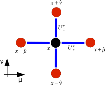
Figure 1: The nearest neighbor stencil part of the lattice Dirac operator $D$, as defined in (2), in the $\mu-\nu$ plane. The color-spinor fields are located on the sites. The SU(3) color matrices $U^{\mu}_{x}$ are associated with the links. The nearest neighbor nature of the stencil suggests a natural even-odd (red-black) coloring for the sites.

Since $M$ is a large sparse matrix, an iterative Krylov solver is typically used to obtain solutions to (1), requiring many repeated evaluations of the sparse matrix-vector product. The matrix is non-Hermitian, so either Conjugate Gradients [7] on the normal equations (CGNE or CGNR) is used, or more commonly, the system is solved directly using a non-symmetric method, e.g., BiCGstab [8]. Even-odd (also known as red-black) preconditioning is used to accelerate the solution finding process, where the nearest neighbor property of the $D_{x,x^{\prime}}$ matrix (see Fig. 1) is exploited to solve the Schur complement system [9]. This has no effect on the overall efficiency since the fields are reordered such that all components of a given parity are contiguous. The quark mass controls the condition number of the matrix, and hence the convergence of such iterative solvers. Unfortunately, physical quark masses correspond to nearly indefinite matrices. Given that current leading lattice volumes are $32^{3}\times 256$, for $>10^{8}$ degrees of freedom in total, this represents an extremely computationally demanding task.

III Graphics Processing Units

In the context of general-purpose computing, a GPU is effectively an independent parallel processor with its own locally-attached memory, herein referred to as device memory. The GPU relies on the host, however, to schedule blocks of code (or kernels) for execution, as well as for I/O. Data is exchanged between the GPU and the host via explicit memory copies, which take place over the PCI-Express bus. The low-level details of the data transfers, as well as management of the execution environment, are handled by the GPU device driver and the runtime system.

It follows that a GPU cluster embodies an inherently heterogeneous architecture. Each node consists of one or more processors (the CPU) that is optimized for serial or moderately parallel code and attached to a relatively large amount of memory capable of tens of GB/s of sustained bandwidth. At the same time, each node incorporates one or more processors (the GPU) optimized for highly parallel code attached to a relatively small amount of very fast memory, capable of 150 GB/s or more of sustained bandwidth. The challenge we face is that these two powerful subsystems are connected by a narrow communications channel, the PCI-E bus, which sustains at most 6 GB/s and often less. As a consequence, it is critical to avoid unnecessary transfers between the GPU and the host. For single-GPU code, the natural solution is to carry out all needed operations on the GPU; in the QUDA library, for example, the linear solvers are written such that the only transfers needed are the initial upload of the source vector to the GPU and the final download of the solution, aside from occasional small messages needed to complete global sums. A multi-GPU implementation, however, cannot avoid frequent large data transfers, and so the challenge becomes to overlap the needed communication with useful work. This is exacerbated further if one wishes to take advantage of many GPUs spread across multiple nodes, since the bandwidth provided the fastest available interconnect, QDR InfiniBand, is half again that provided by (x16) PCI-E.

		GB/s	Gflops		GiB
Card	Cores	Bandwidth	32-bit	64-bit	RAM
GeForce 8800 GTX	128	86.4	518	N/A	0.75
Tesla C870	128	76.8	518	N/A	1.5
GeForce GTX 285	240	159	1062	88	1.0 - 2.0
Tesla C1060	240	102	933	78	4.0
GeForce GTX 480	480	177	1345	168	1.5
Tesla C2050	448	144	1030	515	3.0

TABLE I: Specifications of representative NVIDIA graphics cards.

We turn now to the architecture of the GPU itself. Our purpose is only to highlight those features that have directly influenced our implementation. We focus here on cards produced by NVIDIA and specifically on the GT200 generation, as typified by the Tesla C1060 and the GeForce GTX 285, since the latter will serve as our test bed. The GT200 series is the second of the three extant generations of CUDA-enabled cards, representative examples of which are listed in Table I. The most recent generation, embodying NVIDIA’s “Fermi” architecture, is only now becoming available in mid-2010. We note that while hardware features and performance differ between generations, these have relatively little impact on our multi-GPU strategy. Likewise, most of the considerations we discuss would apply even to an OpenCL implementation targeting graphics cards produced by AMD/ATI.

GPUs support a single-program multiple-data (SPMD) programming model with up to thousands of threads in flight at once. Each thread executes the same kernel, using a unique thread index to determine the work that should be carried out. The GPU in the GeForce GTX 285 card consists of 240 cores organized into 30 multiprocessors of 8 cores each. Each core services multiple threads concurrently by alternating between them on successive clock cycles, so a group of 32 threads (a warp in NVIDIA’s parlance) is executing on the multiprocessor at a given moment. At the same time, many additional threads (ideally hundreds) are typically resident on the multiprocessor and ready to execute. This allows the multiprocessor to swap in a new set of 32 threads when a given set stalls – while waiting for a memory access to complete, for example. In order to hide latency, it is desirable to have many threads resident at once, but each such thread requires a certain number of registers and quantity of shared memory, which limits the total. Just as on a CPU, a register is where a variable is stored while it is being operated on or written out. Registers are not shared between threads. Shared memory, on the other hand, may be shared between threads executing on the same multiprocessor. Strictly speaking, the threads must belong to the same thread block, a group of threads whose size is specified by the programmer; each thread block must consist of a multiple of 64 threads, and one or more thread blocks may be active on a multiprocessor at a time. The GeForce GTX 285 provides 16,384 single-precision registers (8,192 in double precision) and 16 KiB of shared memory per multiprocessor.

The CUDA programming model treats the threads within a block as independent threads of execution, as though they were executing on cores that were true scalar processors; threads may take independent code paths, read arbitrary locations in memory, and so on. In order to obtain optimal performance, however, it is better to treat the multiprocessor as a single 32-lane or 16-lane SIMD unit. This follows from two considerations. First, when threads within a set of 32 (a warp) take different paths at a branch, the various paths are serialized and executed one after another, a condition known as “warp divergence.” Second, when accessing device memory, maximum bandwidth is achieved only when 16 threads access contiguous elements of memory, where each such element is a 4-byte, 8-byte, or 16-byte block. (The CUDA C language defines various short vector types for this purpose, e.g., float2, float4, double2, short4, etc.) This allows the transfer to proceed as a single “coalesced” memory transaction. As described in Section V below, this consideration directly influences the layout of our data.

An additional consideration has to do with the physical organization of the device memory. Like many classic vector architectures but unlike commodity CPUs, GPUs are equipped with a very wide memory bus (512-bit on the GTX 285) with memory partitioned into multiple banks (eight on the GTX 285). Successive 256-byte regions in device memory map to these partitions in a round-robin fashion. This organization is generally transparent to the programmer, but if memory is accessed with a stride that results in traffic to only a subset of the partitions, performance will be lower than if all partitions were stressed equally. Such “partition camping” can result in an unexpected loss of performance for certain problem sizes [10]. As discussed in [4] and Section V below, this was found to be a problem for certain lattice volumes in our LQCD application, with the solution being to pad the relevant arrays to avoid the camping.

To summarize, the GPU memory hierarchy consists of globally-accessible device memory and local per-multiprocessor shared memory, often used as a manually-managed cache, as well as local registers. In addition, GPUs such as the GTX 285 provide two special-purpose caches. The first is a read-only texture cache, which speeds up reads from device memory for certain kinds of access patterns. It also provides various addressing modes and rescaling capability. As described further in Section V, we take advantage of the latter in our half-precision implementation. Finally, each multiprocessor provides a small constant cache (8 KiB on the GTX 285), which is useful for storing run-time parameters and other constants, accessible to all threads with very low latency.

IV Related Work

GPUs were first used to perform LQCD calculations in [11]. This pioneering study predated various programmability improvements, such as the C for CUDA framework, and hence was implemented using the OpenGL graphics API. It targeted single GPU devices. The QUDA library [3] was discussed extensively in [4, 12], where the primary techniques and algorithms for maximizing the efficient use of memory bandwidth were presented for a single GPU device. LQCD on GPUs has also been explored in [13], which focused on questions of fine grained vs. coarse grained parallelism on single GPU devices. In addition, there are several as yet unpublished efforts aimed at exploiting GPUs for LQCD underway.

LQCD has also been implemented on other heterogeneous devices, primarily on the Cell Broadband Engine. Efforts in this direction have been reported in [14, 15] as part of the “QCD Parallel Computing on the Cell Broadband Engine” (QPACE) project and elsewhere [16, 17].

Outside the context of LQCD, general challenges of implementing message passing on heterogeneous architectures have been considered for GPUs in [18] and for the RoadRunner supercomputer in [19]. An effort to provide a general message passing framework utilizing CUDA, MPI, and POSIX threads is also underway at Jefferson Laboratory [20].

V QUDA

The QUDA library is a publicly available collection of optimized QCD kernels built on top of the CUDA framework, with a simple C interface to allow for easy integration with LQCD application software. Currently, QUDA provides highly optimized CG and BiCGstab linear solvers for a variety of different discretizations of the Dirac operator, as well as other time critical components.

V-A General Strategy

The power of GPUs may only be brought to bear when a large degree of parallelism is available. LQCD is fortunate in this regard, since parallelism can easily be achieved by assigning one thread to each lattice site. The mapping from the linear thread index to the 4-dimensional spacetime index is easily obtained through integer division and modular arithmetic involving the lattice dimensions. These runtime parameters (and others, such as boundary conditions) are stored in the constant cache.

In applying the lattice Dirac operator, each thread is thus responsible for gathering its eight neighboring spinors (24 numbers apiece), applying the appropriate spin projector for each, multiplying by the color matrix connecting the sites (18 numbers), and accumulating the results together with the local spinor (24 numbers) weighted by the mass term. The Wilson-clover discretization also requires an extra multiplication by the clover matrix (72 numbers) before the result (24 numbers) is saved to memory. In total, the application of the Wilson-clover matrix requires 3696 floating point operations for every 2976 bytes of memory traffic in single precision (assuming kernel fusion to minimize memory traffic).

V-B Field Ordering

The ordering typical on a CPU is to place the spacetime dimensions running slowest, with internal dimensions (color, spin, and real/imaginary) running fastest. However, since memory coalescing is only achieved if adjacent threads load consecutive blocks of 4, 8, or 16 bytes, the fields must be reordered to ensure this condition. This can be achieved if we abandon the naive ordering,

$$i_{old}=xN_{int}+n,$$ (3)

in favor of the new mapping

$$i_{new}=N_{vec}\left(V\left\lfloor\frac{n}{N_{vec}}\right\rfloor+x\right)+n\,\mbox{mod}\,N_{vec}.$$ (4)

Here $V$ is the spacetime volume; $x$ is the linear spacetime index running from 0 through $V-1$; $n$ corresponds to the internal index running from 0 through $N_{int}-1$, with $N_{int}=$ 24, 12, and 72 elements for the spinor, color (see Section V-C1), and clover fields respectively; and $N_{vec}$ is the length of the vector type used (e.g., $N_{vec}=1,2,4$ for float, float2, and float4). We have found that using $N_{vec}=4$ and $N_{vec}=2$ is optimal in single and double precision, respectively, each corresponding to a length of 16 bytes.

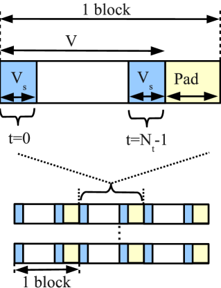
Figure 2: The field ordering used in QUDA: $N_{int}V$ numbers are broken up into $N_{int}/N_{vec}$ blocks of $V$ short vectors ( $=N_{vec}V$ numbers). Successive threads thus read successive short vectors ensuring coalescing of the memory transfers. Within a block the time index runs slowest, implying that the two faces on the temporal boundaries are each contiguous within the block; each face is stored in $V_{s}$ vectors. The blocks are separated by a padding region to avoid partition camping. As an example, in single precision one would use the float4 vector type ($N_{vec}=4$), and thus 6 blocks would be needed to store the $24V$ numbers that make up a color-spinor. Likewise, in 2-row storage, the gauge field would need 3 blocks to store the $12V$ numbers needed for each direction $\mu$. With 4 such directions, altogether 12 blocks are needed to store all the link matrices. With the size of the padding chosen to be $V_{s}=XYZ$ sites, the ghost zone of link matrices $U^{\mu}_{x-\hat{\mu}}$ can be hidden entirely in the padding.

QUDA follows the usual lattice site assignment for the color matrices. The color matrix connecting sites $x$ and $x+\hat{\mu}$ is denoted by $U_{x}^{\mu}$ and stored at lattice site $x$. It follows that $U_{x-\hat{\mu}}^{\mu}$, which is required for the gather from the backwards direction for site $x$, is stored at site $x-\hat{\mu}$. (The matrix conjugation is performed at no cost through register relabeling in the kernel.)

As anticipated in Section III, for certain problem sizes performance may be affected by partition camping. The simple solution QUDA takes to this problem is to pad the gauge, spinor, and clover fields by one spatial volume, $V_{s}=XYZ$, so that the linear indexing is given by

$$i=N_{vec}\left((T+1)V_{s}\left\lfloor\frac{n}{N_{vec}}\right\rfloor+x\right)+n\,\mbox{mod}\,N_{vec}.$$ (5)

Here $X$, $Y$, $Z$ and the $T$ are the lengths of the respective spacetime dimensions, with $V=V_{s}T$. Although not originally intended for this purpose, padding the fields by an extra spatial volume is also convenient for the parallelization process (see Section VI). We illustrate the field ordering in Fig. 2.

V-C Reducing Memory Traffic

Given the peak instruction and bandwidth throughputs of current GPUs (Table I), evaluation of the Wilson-clover matrix vector product is strongly bandwidth bound. The approach taken by QUDA is to minimize memory traffic, even at the expense of additional floating point operations, to accelerate performance using the following techniques:

V-C1 Gauge field compression

Only the first two rows of the color matrices are stored in device memory, and using unitarity, the third row is reconstructed in registers from the complex conjugate of the cross product of the first two rows.

V-C2 Similarity transformations

Physically motivated similarity transformations are employed to increase the sparsity of the matrix. In particular, the spin projectors in the temporal dimension $P^{\pm 4}$ are diagonalized by changing from the conventional chiral basis to a “non-relativistic” basis,

$$P^{\pm 4}=\left(\begin{array}[]{rrrr}1&0&\pm 1&0\\ 0&1&0&\pm 1\\ \pm 1&0&1&0\\ 0&\pm 1&0&1\\ \end{array}\right)\Longrightarrow$$ (6)

$$P^{+4}=\left(\begin{array}[]{rrrr}2&0&0&0\\ 0&2&0&0\\ 0&0&0&0\\ 0&0&0&0\\ \end{array}\right),P^{-4}=\left(\begin{array}[]{rrrr}0&0&0&0\\ 0&0&0&0\\ 0&0&2&0\\ 0&0&0&2\\ \end{array}\right).$$

This has the benefit that only 12 real numbers need be loaded when gathering neighboring spinors in the temporal direction and also aids our parallelization approach (See Section VI).

V-C3 Precision Truncation

Further acceleration is obtained through the use of 16-bit fixed point storage, from here on referred to as half precision. This is implemented by reading the gauge field and spinor field elements via the texture cache, using the read mode cudaReadModeNormalizedFloat. When a texture reference is defined using this mode, a signed 16-bit (or even 8-bit) integer read in from device memory will be automatically converted to a 32-bit floating point number in the range $[-1,1]$. This format is immediately suitable for the color matrices since all of their elements lie exactly in this range, as a consequence of unitarity. The spinors require an extra normalization, which is shared between all elements of a single spinor. Thus in half precision a spinor is stored as 6 short4 arrays and a single float normalization array.

V-D Mixed-precision Linear Solvers

The use of mixed-precision iterative refinement for solving linear equations is fairly commonplace on GPUs and other architectures where the use of double precision comes with a significant performance penalty. Such an approach allows the bulk of the computation to be performed in fast low precision, with periodic updates in high precision to ensure accuracy of the final solution. Even on architectures where there is parity between peak single and double precision performance, a factor of two difference in memory traffic is unavoidable, and so for bandwidth-bound problems such as our sparse matrix-vector product, the use of mixed precision remains advantageous. QUDA uses a variant of reliable updates [21] to implement mixed-precision iterative refinement. This approach has the advantage that a single Krylov space is preserved throughout the solve, as opposed to the traditional approach of defect correction which explicitly restarts the Krylov space with every correction, increasing the total number of solver iterations [4]. It was found that the best time to solution is typically obtained using either double-half or single-half approaches.

V-E Auto-tuned Linear Algebra Kernels

QUDA provides the additional vector-vector linear algebra (BLAS1-like) kernels needed to implement the linear solvers. These additional routines take advantage of kernel fusion wherever possible to reduce memory traffic and hence improve performance of the complete solver. Since each of these kernels and their various half, single, and double precision variants may have different optimal CUDA parameters (i.e., sizes of the thread blocks and the number of blocks treated at once), an auto-tuning approach is taken to ensure maximum performance. All possible combinations of parameters are tested for each kernel, and the optimal values are written out to a header file for inclusion in production code after a recompilation of the library. Due to the memory bandwidth intensity of these (essentially streaming) kernels, the complete solver typically runs 10 to 20% slower than would the matrix-vector product in isolation.

VI Multi-GPU Implementation

VI-A General Strategy

In parallelizing across multiple GPUs, we have taken the simplest approach by only dividing the time dimension, with the full extent of the spatial dimensions confined to a single GPU. This approach was motivated by the asymmetric nature of the lattice dimensions under study ($24^{3}\times 128$ and $32^{3}\times 256$), and in order to simplify this initial parallelization. In this form, since we are parallelizing over the slowest running spacetime index, the changes required to the single GPU kernel code were relatively minimal. If one were to attempt to scale to hundreds of GPUs or more, multi-dimensional parallelization would clearly be needed to keep the local surface to volume ratio under control. Given current lattice sizes, however, such extreme parallelization would imply small local volumes and require rethinking of the fundamental algorithms. Work in this direction is underway.

For parallelizing across multiple GPUs, each GPU can either be controlled using a distinct CPU thread or with a distinct process. The potential advantage of the threaded approach is that it avoids unnecessary copies within a node; however, this advantage has decreased on recent CPUs that feature integrated memory controllers and much higher memory bandwidth (compared to pre-Nehalem Xeons, for example), reducing the overhead of an additional local memory copy. To communicate between GPUs on different nodes, a message passing approach is necessary since the memory space is by definition separate. While mixed-mode programming is possible (threads within a node, message passing between the nodes), we exclusively used a message passing approach since initial investigations suggested no improvement would be gained from the use of threads. In particular, we used QMP (QCD Message Passing) which is an API built on top of MPI that provides convenient functionality for LQCD computations [22].

In parallelizing the action of the Wilson-clover matrix onto a spinor field partitioned between $N$ distinct GPUs, we slice the temporal dimension into $N$ equal sized volumes of size $V/N=V_{s}T/N$. Referring to (2), the only part of the matrix that connects different lattice sites is the action of $D_{x,x^{\prime}}$, since the clover matrix $A_{x}$ is local to a given lattice site. When updating the sites on either end of the local temporal boundary, the adjacent spinors which are on the neighboring GPUs are required, as well as the gauge field matrix connecting these sites.

VI-B Gauge Field Ghost Zone

The link matrix $U_{x}^{\mu}$ connecting sites $x$ and $x+\hat{\mu}$ is stored at site $x$; hence the required link matrix for the receive from the forward temporal direction for sites in the last spatial volume (or timeslice) will already be present locally, and only the adjacent spinor is required. For the receive from the backward temporal direction into the first timeslice, the required link matrix will be on the adjoining GPU and so must be transferred. Since the link matrices are constant throughout the execution of the linear solver, we transfer the adjoining link matrices in the program initialization. Compared to the original single GPU code, this posed the obvious question: where should the extra face (the ghost zone) of gauge field matrices be stored? Given that the fields were already padded by an extra spatial volume, a very natural location is within the padded region since this is exactly the correct size to store the additional gauge field slice (see Fig. 2). Altering the kernel for this change simply required that if the thread id corresponded to the first timeslice (local to the GPU) then the gauge field array indices are set to the padded region. Extra constants were introduced to describe the boundary conditions at the start and end of the local volume, since one of these boundaries might correspond to a global boundary and not just a local boundary.

VI-C Spinor Field Ghost Zone

Our initial strategy for storing the transferred faces was to put them in the padded regions of the destination GPU’s spinor field. Like the gauge field ghost zone this seems very natural, but it introduced complications into the reduction kernels used in the Krylov solvers: these assume a contiguous memory buffer, and so without careful rewriting the ghost zones would be double counted. The approach we opted for instead was to oversize the spinor fields by the size of the two transferred faces. When doing reductions, this end zone can be simply excluded ensuring correctness. As described in Section V-C2 the spin projectors in the temporal direction are diagonalized, halving the amount of data that needs to be transferred in the temporal gathering, and so the extra total storage required is actually only $24V_{s}$ components. The upper 12 spinor components which arise from the receive from the backward direction occupy the first half of the end zone, and the lower 12 spinor components arising from the receive from the forward direction occupy the second half. For half precision the extra normalization constant for each (12 component) spinor is also required, and hence an end zone of size $2V_{s}$ elements is added to the normalization field. We illustrate the spinor ghost zones and the basic communication requirements in Fig. 3.

With the ghost zone elements stored in the end zone, extra indexing logic was required to ensure that the correct spinors would be loaded by the threads updating the boundaries. Fortunately, this extra logic introduced minimal overhead since warp divergence is avoided because the number of spatial sites $V_{s}$ is divisible by the warp size, a condition that is met by the lattice dimensions under consideration here (and all production LQCD calculations that we aware of).

VI-D Communication Strategies

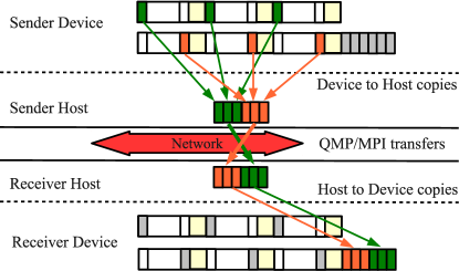
Figure 3: Spinor ghost zones and communication steps: We show the source spinor on the sending device (top) assuming $N_{vec}=4$, corresponding to 6 blocks from Fig. 2. The grey buffers at the end correspond to the ghost zones. The top 3 blocks correspond to the $P^{+4}$ projected components, while the lower 3 blocks nearer the ghost zone correspond to $P^{-4}$. Data from the back faces (green) needs to be gathered into a communications buffer on the sending host and likewise for the forward face (orange). The faces are then transferred to the receiving host via QMP/MPI. Once transferred the faces are transferred to the ghost zones on the receiving device (bottom of diagram), which then uses the data directly from the ghost zones, hence the corresponding faces have been greyed out.

VI-D1 No Overlap

The first and simplest approach to parallelization is to perform all of the communications up front and then do the computation for the entire volume in a single kernel. The device-to-host transfers are achieved through the use of separate cudaMemcpy calls (one for each face block), with half precision requiring an extra cudaMemcpy for the face of the normalization array. Once on the host, all of these blocks are contiguous in memory, allowing for a single message passing in each direction. The received faces are sent to the device using a single cudaMemcpy for each face (with an extra cudaMemcpy required for each of the normalization faces in half precision) and placed in the end zone of the spinor field. Finally the Wilson-clover kernel is executed.

VI-D2 Overlapping Communication and Computation

Our second implementation aimed to overlap all of the communication with the computation of the internal volume. To do so, the CUDA streaming API was used, which allows for a CUDA kernel to execute asynchronously on the GPU at the same time that data is being transferred between the device and host using cudaMemcpyAsync.

Additionally this makes use of non-blocking MPI communication possible: after the backward face has been transferred to the host, the MPI exchange of this face to its neighbor is overlapped with the transfer of the forward face from device to host. In turn, when the first face has been received, this can be sent to the device while the second face is being communicated. This approach requires three CUDA streams: one to execute the kernel on the internal volume, one for the face send backward / receive forward, and one for the face send forward / receive backward. An additional required step is that the streams responsible for gathering the faces to the host must be synchronized, using cudaStreamSynchronize, before message passing can take place to ensure transfer completion. In principle, we could also overlap the host-to-device transfer of the second face and the computation involving the first face. This would yield a minimal speedup at best, since the time spent executing the face kernel is not the limiting factor, and it may actually reduce overall performance since the kernel would be updating half as many sites at a time, reducing parallelism and potentially decreasing kernel efficiency.

VI-E Parallelizing the Linear Solver

Aside from the parallelization of the sparse matrix vector product, the only other required addition to the code was the insertion of MPI reductions for each of the linear algebra reduction kernels.

VII Solver Performance Results

VII-A Details of the Numerical Experiments

Our numerical experiments were carried out on the “9g” cluster at Jefferson Laboratory. This cluster is made up of 40 nodes containing 4 GPUs each, as well as an additional 16 nodes containing 2 GPU devices each that are interconnected by QDR InfiniBand on a single switch. In this study, we focused our attention primarily on the partition made up of the 16 InfiniBand connected nodes, with one or two exceptions. The nodes themselves utilize the Supermicro X8DTG-QF motherboard populated with two Intel Xeon E5530 (Nehalem) quad-core processors running at 2.4 GHz, 48 GiB of main memory, and two NVIDIA GeForce GTX 285 cards with 2 GiB of device memory each.

The nodes run the CentOS 5.4 distribution of Linux with version 190.29 of the NVIDIA driver. The QUDA library was compiled with CUDA 2.3 and linked into the Chroma software system using the Red Hat version 4.1.2-44 of the GCC/G++ toolchain. Communications were performed using version 2.3.2 of the QCD Message Passing library (QMP) built over OpenMPI 1.3.2. In all our tests we ran in a mode with one MPI process bound to each GPU.

The numerical measurements were taken from running the Chroma propagator code and performing 6 linear solves for each test (one for each of the 3 color components of the upper 2 spin components), with the quoted performance results given by averages over these solves. Statistical errors were also determined but are generally too small to be seen clearly in the figures. Importantly, all performance results are quoted in terms of “effective Gflops” that may be compared with implementations on traditional architectures. In particular, the operation count does not include the extra work done to reconstruct the third row of the link matrix.

We carried out both strong and weak scaling measurements. The strong scaling measurements used lattice sizes of $V=24^{3}\times 128$ and $V=32^{3}\times 256$ sites respectively. Both the lattice sizes and the Wilson-clover matrix had their parameters chosen so as to correspond to those in current use by the Anisotropic Clover analysis program of the Hadron Spectrum collaboration. The lattices used were weak field configurations. Such configurations are made by starting with all link matrices set to the identity, mixing in a small amount of random noise, and re-unitarizing the links to bring the links back to the $SU(3)$ manifold. We emphasize that while these lattices were not physical, we have tested the code on actual production lattices on both the volumes mentioned for correctness. The concrete physical parameters do not affect the rate at which the code executes but control only the number of iterations to convergence in the solver. The weak scaling tests utilized local lattice sizes of $V=32^{4}$ and $V=24^{3}\times 32$ sites per GPU, respectively.

The solver we employed was the reliably updated BiCGstab solver discussed in [4]. We ran the solver in single precision and mixed single-half precision with and without overlapped communications in the linear operator. For the lattices with $V_{s}=24^{3}$ spatial sites, we also ran the solver in uniform double precision and in mixed double-half precision modes. When run in single or single-half mixed precision modes the target residuum was $||r||=10^{-7}$, whereas in the double precision and mixed double-half precision modes the residuum was $||r||=10^{-14}$. In addition, the delta parameter was set to $\delta=10^{-3}$ in single, $\delta=10^{-1}$ in mixed single-half, $\delta=10^{-5}$ in double and $\delta=10^{-2}$ in the mixed double-half modes of the solver respectively. The meanings of these parameters are explained fully in [4].

VII-B Weak Scaling

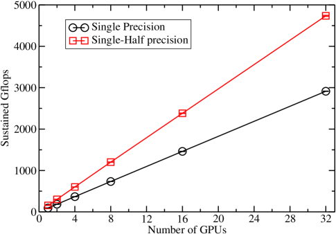
(a)

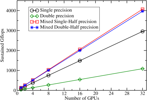
(b)

Figure 4: Weak scaling results for up to 32 GPUs on lattices with local volumes of (a) $V=32^{4}$ and (b) $V=24^{3}\times 32$ sites per GPU. In subfigure (a) we show performance results for the single precision solver and the mixed single-half precision solver. In subfigure (b) we also show results for double precision and mixed double-half precision. In both (a) and (b), the data come from solvers where communications and computation have been overlapped, as this performed fastest in weak scaling tests.

Our results for weak scaling are shown in Fig. 4. We see near linear scaling on up to 32 GPUs in all solver modes. In the case with $V=32^{4}$ sites per GPU, we were unable to fit the double precision and mixed double-half precision problems into device memory, and hence we show only the single and single-half data. In the case with local volume of $24^{3}\times 32$ we show also double precision and mixed double-half precision data. It is gratifying to note that the mixed double-half precision performance of Fig. 4(b) is nearly identical to that of the single-half precision case. Both mixed precision solvers are substantially more performant than either the uniform single or the uniform double precision solver. We note that for lattices with $32^{4}$ sites per GPU we have reached a performance of 4.75 Tflops.

VII-C Strong Scaling

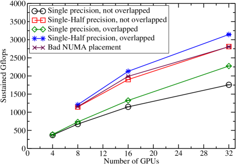
(a)

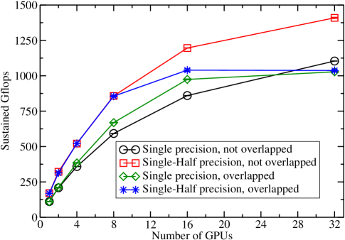
(b)

Figure 5: Strong scaling results for up to 32 GPUs on lattices with total volumes of (a) $V=32^{3}\times 256$ sites and (b) $V=24^{3}\times 128$ sites. We show data for single precision without overlapping communications and computation (black), mixed single-half precision without overlapping communications and computation (red), single precision with overlapped communications and computation (green), and mixed single-half precision with overlapped communications and computation (blue). In subfigure (a) we also show mixed single-half precision with overlapped communications but with deliberately bad NUMA placement (maroon).

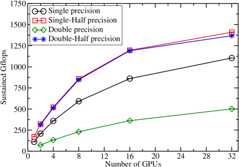
Figure 6: Strong scaling results for the $V=24^{3}\times 128$ lattice in single precision, double precision, single-half mixed precision, and double-half mixed precision. We used the solver that did not overlap computations and communications for these results, since as shown in Fig. 5 it was faster than the overlapped solver for the $V=24^{3}\times 128$ lattice in single and mixed single-half precisions.

Fig. 5 shows our strong scaling results. In Fig. 5(a) we show the data for the lattices with $V=32^{3}\times 256$ sites. We see a clear deviation from linear scaling as the number of GPUs is increased and the local problem size per GPU is reduced. This is not unexpected, since as the number of GPUs is increased the faces represent a larger fraction of the overall work. The improvement from overlapping communication with computation is increasingly apparent as the number of GPUs increases. The benefits of mixed precision over uniform single precision can clearly be seen. However, we note that performing the mixed precision computation comes with a penalty in terms of memory usage: the mixed precision solver must store data for both the single and half precision solves, and this increase in memory footprint means that at least 8 GPUs are needed to solve this system. The uniform single precision solver requires only the single precision data and can be solved (at a performance cost) already on 4 GPUs. We highlight the fact that the 32 GPU system is made up of 16 cluster nodes, which themselves contain 128 Nehalem cores. We have performed a solution of this system on the Jefferson Lab “9q” cluster, which is identical in terms of cores and InfiniBand networking but does not contain GPUs. On a 16-node partition of the “9q” cluster we obtained 255 Gflops in single precision using highly optimized SSE routines, which corresponds to approximately 2 Gflops per CPU core. In our parallel GPU computation, on 16 nodes and 32 GPUs we sustained over 3 Tflops which is over a factor of 10 faster than observed without the GPUs.

Fig. 5(b) shows our strong scaling results for the lattice with $V=24^{3}\times 128$ sites. This lattice has half the time extent of the larger lattice, and thus we expect strong scaling effects to be noticeable at smaller GPU partitions than in the previous case. Further, the spatial volume is a factor of $2.3$ smaller for the $V=24^{3}\times 128$ lattices than for the larger case. We were surprised that the trend in our results is different from that in Fig. 5(a). Notably, in this case we seem to gain little from overlapping communication and computation in the mixed precision solver. Indeed, for more than 8 GPUs the mixed precision performance reaches a plateau and is surpassed even by the purely single precision case. We believe this dropoff in the strong scaling is due to additional overheads incurred in overlapping communications with computations arising from system and driver issues. We will return to this point in Section VII-D, where we discuss latency microbenchmarks, but suffice it to say that using cudaMemcpyAsync appears to have a higher latency than cudaMemcpy. This may be a feature of our motherboard or the version of the NVIDIA driver we are using. In the case of the $V=32^{3}\times 256$ lattice, probably the volume in the body is large enough to hide this extra latency. In the case of the $V=24^{3}\times 128$ lattice, our data suggests that the local volume may be sufficiently small that the overhead of setting up the asynchronous transfers dominates and that in this instance the lower latency of synchronous cudaMemcpy calls can result in better performance.

Fig. 6 shows the strong scaling data for various precision combinations for the $V=24^{3}\times 128$ lattice, where we now include uniform double and mixed double-half precision results and do not overlap communication with computation. Again we see that the mixed precision solvers employing half precision outperform both single and double uniform precision solvers. Note that uniform double precision exhibits the best strong scaling of all because this kernel is less bandwidth bound due to the much lower double precision peak performance of the GTX 285 (see Table I).

VII-D System Issues

The PCI-E architecture in our Supermicro nodes was such that the two GPU devices were each on a bus with a direct connection to a separate socket on the motherboard. In our tests we launched two MPI processes per node. In order to obtain maximum bandwidth on the buses, it was necessary to explicitly bind each MPI process to the correct socket. We accomplished this using the processor affinity feature of OpenMPI.

In Fig. 5(a) we show the performance a deliberately badly chosen NUMA configuration (with maroon x-symbols). We bound each process to the opposite socket from the CUDA device it was using. One can see that the performance is noticeably lower than the correctly bound case denoted by blue asterisks in Fig. 5(a).

Secondly, as alluded to previously, we note that on these nodes the latencies of cudaMemcpy (used in the non-overlapped communication code) and of cudaMemcpyAsync (followed immediately by a cudaSynchronizeThread) call are quite different.

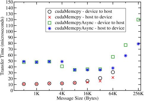
Figure 7: Latency microbenchmark showing tranfer times from host to device or vice versa for messages of varying sizes. We show data for: device to host using cudaMemcpy (black), host to device using cudaMemcpy (red), device to host using cudaMemcpyAsync + cudaSynchronizeThreads (green) and host to device using cudaMemcpyAsync+cudaSynchronizeThreads (blue). The timings are taken over 500,000 message transfers

As shown in Fig. 7, using cudaMemcpyAsync incurs a latency of just under 50 microseconds whereas a synchronous cudaMemcpy has a much shorter latency of 11 microseconds. It can also be seen that once out of the latency limited region, the graphs show different gradients for the host-to-device and device-to-host transfers, indicating different host-to-device and device-to-host bandwidths. These features may depend somewhat on the version of the NVIDIA driver and motherboard BIOS used, but additional testing so far suggests that the main culprit is a hardware limitation in the early revision of the Intel 5520 (Tylersburg) chipset used in the nodes. Therefore the decision on whether to overlap communication and computation or not may depend on the system under consideration, as well as the problem size.

VIII Conclusion and Future Work

We have demonstrated what we believe is the first successful attempt to use multiple GPU units in parallel for LQCD computations. We have weak scaled our application to 4.75 Tflops on 32 GPUs and have strong scaled the application, on a problem size of scientific interest, to over 3 TFlops. In this latter case, we have achieved over a factor of 10 increase in performance compared to not using GPUs (255 Gflops on a “regular” cluster partition containing the same number processors). We believe that the order of magnitude increase in computing power is an enabling technology for sophisticated modern analysis methods of great interest to particle and nuclear physics. Indeed the solver we have described is now in use in production LQCD calculations of the spectrum of hadrons using the technique of distillation [2, 23]. Current calculations use lattice configurations of the same size as described in Section VII which were generated on leadership computing platforms under DOE INCITE and NSF TeraGrid allocations (granted to the USQCD and Hadron Spectrum collaborations, respectively). The calculations involve 32768 calls to the solver for each configuration and benefit enormously from the speedup delivered by the GPU solver.

Prior to parallelizing the QUDA library, our larger volume dataset was not amenable to solution on GPUs due to memory constraints. The use of multiple GPUs allows the solution to proceed, realizing the large increases in cost effectiveness promised by GPUs.

A slightly more nuanced point is that the nodes containing 4 GPUs (and no InfiniBand) may now be more efficiently utilized. Prior to parallelization, one could solve the $24^{3}\times 128$ problem on a single GPU and analyze two configurations simultaneously on a single node. One could not analyze more, due to the limitations on the host (primarily memory capacity). Now one can analyze 2 configurations simultaneously using 2 GPUs each, optimally utilizing all 4 GPUs in the node. The exact optimization of a node configuration in terms of InfiniBand cards, GPUs, and operating model is an interesting issue but is beyond the scope of this paper.

There are many avenues for future exploration. Currently only the solvers have been accelerated in the QUDA library. Parallelization onto multiple GPUs may make gauge generation on GPU clusters an interesting and desirable possibility. We are also interested in porting more modern algorithms to the GPUs such as the adaptive multigrid solver discussed in [24] to speed up computations even further. We follow the development of the OpenCL standard with interest with a view to potentially harness GPU devices from AMD as well as NVIDIA, and we await future hardware and software improvements to allow better coexistence of GPUs and message-passing (such as sharing pinned memory regions between CUDA and MPI). Finally, we hope that the lessons learned from GPUs will be usefully applicable on heterogeneous systems in general as we head towards the exascale.

References

- [1] R. Babich, R. Brower, M. Clark, G. Fleming, J. Osborn, and C. Rebbi, “Strange quark content of the nucleon,” Proc. Science (LATTICE2008), 2008, 160 [arXiv:0901.4569 [hep-lat]].
- [2] M. Peardon et al. [Hadron Spectrum Collaboration], “A novel quark-field creation operator construction for hadronic physics in lattice QCD,” Phys. Rev. D, vol. 80, 2009, p. 054506 [arXiv:0905.2160 [hep-lat]].
- [3] http://lattice.bu.edu/quda
- [4] M. A. Clark, R. Babich, K. Barros, R. C. Brower, and C. Rebbi, “Solving Lattice QCD systems of equations using mixed precision solvers on GPUs,” Comput. Phys. Commun., vol. 181, 2010, p. 1517. [arXiv:0911.3191 [hep-lat]].
- [5] R. G. Edwards and B. Joo [SciDAC Collaboration and LHPC Collaboration and UKQCD Collaboration], “The Chroma software system for lattice QCD,” Nucl. Phys. Proc. Suppl., vol. 140, 2005, p. 832 [arXiv:hep-lat/0409003].
- [6] B. Sheikholeslami and R. Wohlert, “Improved Continuum Limit Lattice Action For QCD With Wilson Fermions,” Nucl. Phys. B, vol. 259, 1985, p. 572.
- [7] M. R. Hestenes and E. Stiefel, “Methods of Conjugate Gradients for Solving Linear Systems”, J. of Research of the National Bureau of Standards, vol. 49, no. 6, 1952, p. 409.
- [8] H. A. van der Vorst, “BI-CGSTAB: a fast and smoothly converging variant of BI-CG for the solution of nonsymmetric linear systems”, SIAM J. Sci. Stat. Comput., vol. 13, no. 2, 1992, pp. 631–644.
- [9] T. A. DeGrand and P. Rossi, “Conditioning techniques for dynamical fermions,” Comput. Phys. Commun., vol. 60, 1990, p. 211.
- [10] G. Ruetsch and P. Micikevicius, “Optimizing matrix transpose in CUDA,” NVIDIA Technical Report, 2009.
- [11] G. I. Egri, Z. Fodor, C. Hoelbling, S. D. Katz, D. Nogradi, and K. K. Szabo, “Lattice QCD as a video game,” Comput. Phys. Commun., vol. 177, 2007, p. 631 [arXiv:hep-lat/0611022].
- [12] K. Barros, R. Babich, R. Brower, M. A. Clark, and C. Rebbi, “Blasting through lattice calculations using CUDA,” Proc. Science (LATTICE2008), 2008, 045 [arXiv:0810.5365 [hep-lat]].
- [13] K. Z. Ibrahim and F. Bodin, and O. Pene, “Fine-grained Parallelization of Lattice QCD Kernel Routine on GPU”, J. of Parallel And Distributed Computing, vol. 68, no. 10, 2008, pp. 1350–1359.
- [14] F. Belletti et al., “QCD on the Cell Broadband Engine,” Proc. Science (LAT2007), 2007, 039 [arXiv:0710.2442 [hep-lat]].
- [15] H. Baier et al., “QPACE – a QCD parallel computer based on Cell processors,” Proc. Science (LAT2009), 2009, 001 [arXiv:0911.2174 [hep-lat]].
- [16] G. Shi, V. Kindratenko, and S. Gottlieb, “Cell processor implementation of a MILC lattice QCD application,” Proc. Science (LATTICE2008), 2008, 026 [arXiv:0910.0262 [hep-lat]].
- [17] J. Spray, J. Hill, and A. Trew, “Performance of a Lattice Quantum Chromodynamics Kernel on the Cell Processor,” Comput. Phys. Commun., vol. 179, 2008, p. 642 [arXiv:0804.3654 [hep-lat]].
- [18] J. Stuart and J. D. Owens, “Message Passing on Data-Parallel Architectures,” Proc. the 23rd IEEE International Parallel and Distributed Processing Symposium, Rome, Italy, 2009.
- [19] S. Parkin and M. Lang, and D. Kerbyson, “The Reverse-acceleration Model for Programming Petascale Hybrid Systems,” IBM J. of Research and Development, vol. 53, 2009.
- [20] J. Chen and W. Watson, in preparation.
- [21] G. L. G. Sleijpen, and H. A. van der Vorst, “Reliable updated residuals in hybrid Bi-CG methods,” Computing, vol. 56, 141–164 (1996).
- [22] http://usqcd.jlab.org/usqcd-docs/qmp
- [23] J. J. Dudek, R. G. Edwards, M. J. Peardon, D. G. Richards, and C. E. Thomas, “Toward the excited meson spectrum of dynamical QCD,” 2010 [arXiv:1004.4930 [hep-ph]].
- [24] J. Brannick, R. C. Brower, M. A. Clark, J. C. Osborn, and C. Rebbi, “Adaptive Multigrid Algorithm for Lattice QCD,” Phys. Rev. Lett., vol. 100, 2008, 041601 [arXiv:0707.4018 [hep-lat]].