Dephasing of spin and charge interference in helical Luttinger liquids

Abstract

We consider a four-terminal Aharonov-Bohm interference setup formed out of two edges of a quantum spin Hall insulator, supporting helical Luttinger liquids (HLLs). We show that the temperature and bias dependence of the interference oscillations are linked to the amount of spin flips in tunneling between two HLLs which is a unique signature of a HLL. We predict that spin dephasing depends on the electron-electron ($e$-$e$) interaction but differently from the charge dephasing due to distinct dominant tunneling excitations. In contrast, in a spinful Luttinger liquid with SU(2) invariance, uncharged spin excitations can carry spin current without dephasing in spite of the presence of $e$-$e$ interactions.

Quantum spin-Hall (QSH) insulators can support edge states that are topologically protected against disorder, and are present in the absence of a magnetic field kane2005-qsh ; bernevig2006-qsh ; wu2006-hla ; xu2006-soq . These edge states have a special helical structure, in that their direction of propagation is associated with a given value of spin polarization. Evidence of the existence of such helical edge states has been recently found in HgTe based quantum well structures konig2007-qsh ; roth2009-nti . They in principle enable direct control of spin currents via electronic means, which has generated interest in their spintronics applications maciejko2009-sae ; jiang2009-qsh .

However, the fact that spin can be controlled electronically implies that it must also couple to the electron-electron ($e$-$e$) interaction. This is in contrast to SU(2) symmetric systems in which propagating spin excitations can be uncharged, and therefore remain unaffected by Coulomb forces giamarchi2004-qpi . The $e$-$e$ interaction is the dominant cause for dephasing of electronic coherence in low-dimensional mesoscopic systems, at temperatures low enough datta1999-eti , and in 1D systems, this dephasing is associated with fractionalization of excitations lehur2002-efd . In QSH systems, one would therefore expect that dephasing originating from the Coulomb interaction would be visible also in the spin coherence, and lead to fractionalization of spin das2010-sps . On the one hand, this will limit the spin coherence time which may be harmful for some applications, but on the other hand, it can serve as a characteristic signature of the QSH state.

One possible way to probe the coherence in a low-dimensional mesoscopic system is to observe the decay of interference oscillations lehur2005-dom ; *lehur2006-eli. A simple geometry in which this can be done is an Aharonov-Bohm (AB) interferometer, where the phase difference between two paths of propagation is controlled with a magnetic flux. Although such flux would not ordinarily couple to spin currents, the structure of helical edge states makes this possible maciejko2009-sae . Alternatively, one can observe the interference oscillations as a function of gate or bias voltages, or spin density differences, applied to the system — these will be present also in non-helical edge states.

Here, we analyze dephasing of charge and spin interference in an AB interferometer composed of tunnel-coupled interacting helical edge states (see Fig. 1). We find that dephasing in charge tunneling currents depends on the degree of spin-flips in tunneling. Moreover, we establish a direct relationship between charge and spin currents in helical four-probe setups, which translates the results on charge dephasing to apply to spin. Here, helical edge states turn out to differ significantly from ordinary spinful edge states, which in the presence of SU(2) spin symmetry can support interference effects in spin current without dephasing, even when Coulomb interaction is present.

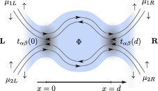
Figure 1: (Color online) Interferometer supporting helical edge states, where the direction of propagation is correlated with the spin ($\uparrow/\downarrow$). The four-terminal setup is connected to noninteracting leads, biased at potentials $\mu_{1/2,L/R}$. Tunneling between the edges occurs at points $x=0$ and $x=d$ (shaded). The loop between the tunneling points is threaded by a magnetic flux $\Phi$.

Model. An interacting helical edge state can be modeled as a helical Luttinger liquid (HLL) wu2006-hla . Each HLL has the same degrees of freedom as a spinless LL (SLLL) with right ($+$) and left ($-$) movers associated with a given spin state ($\lvert+\rangle\,\widehat{=}\lvert\uparrow\rangle$,$\lvert-\rangle\,\widehat{=}\lvert\downarrow\rangle$), so spin is redundant. Microscopically, the spin states $\lvert\uparrow\rangle$ and $\lvert\downarrow\rangle$ refer to Kramers partners which are either electron spin or total angular momentum eigenstates, depending on the material.

The bosonized Hamiltonian for a HLL reads wu2006-hla

$$H_{0}=\frac{v_{F}}{2}\int_{-\infty}^{\infty}\mathrm{d}x\,[g(x)^{-2}:(\partial_{x}\vartheta)^{2}:+:(\partial_{x}\phi)^{2}:]$$ (1)

where the standard boson fields $\vartheta(x)$, $\phi(x)$ satisfy $[\phi(x),\vartheta(x^{\prime})]=(i/2)\mathop{\mathrm{sgn}}(x-x^{\prime})$ and are associated with annihilation operators for left- and right-going electrons, $\psi_{\alpha}(x)\propto e^{i\alpha[k_{F}x+\sqrt{\pi}\vartheta(x)]+i\sqrt{\pi}\phi(x)}$, $\alpha=\pm$, and $g(x)$ is an $e$-$e$ interaction parameter. Moreover, $v_{F}$, $k_{F}$ are the Fermi velocity and Fermi wave vector. For a pair of edge states, the spin-direction mapping is reversed on the second edge. We assume the edge states are contacted to noninteracting Fermi leads a distance $l$ away from the central region. That is, there is a repulsive interaction ($g(x)=g<1$) in the central region ($-l<x<l$), but the leads ($|x|>l$) are noninteracting ($g=1$). Here, we assume that the relevant lead modes coupled to the system are also described by Eq. (1). We will use dimensionless units in which $\hbar=e=k_{B}=1$.

The tunneling between the upper and lower edges is described by the Hamiltonian

$$H_{T}=L\sum_{R=0,d}\sum_{\alpha\beta=\pm}t_{\alpha\beta}(R)\psi_{1,\alpha}(R)^{\dagger}\psi_{2,\beta}(R)+\text{h.c.}\,,$$ (2)

where $j=1,2$ denote the upper and lower edges and $L$ is the total length of an edge (including the leads). Under time-reversal symmetry broken only by the magnetic flux $\Phi$ in the interferometer loop, the tunneling elements read $t_{\alpha\beta}(R)=e^{-2\pi i(R/d)\Phi/\Phi_{0}}t^{\prime}_{\alpha\beta}(R)$, $t^{\prime}_{\alpha\beta}=-\alpha\beta(t_{-\alpha,-\beta}^{\prime})^{*}$, where $\Phi_{0}=h/e$ is the magnetic flux quantum. In the presence of inversion symmetry, spin is conserved bernevig2006-qsh and, as a consequence, the spin-flipping terms should vanish, $t^{\prime}_{++}=t_{--}^{\prime}\simeq 0$. However, local gates vayrynen2010-ema or strain can induce spin-mixing in the tunneling amplitudes, allowing for non-zero $t^{\prime}_{\alpha\alpha}$.

We compute currents in the presence of tunneling, treating $H_{T}$ as a perturbation. This is expected to be valid in HLLs, as at low energies the tunneling stays irrelevant (in the renormalization group sense) for $1/2<g<2$ teo2009-cbo ; hou2009-cja . Bias voltages in terminals are taken into account by assuming that the incoming states have thermal populations described by chemical potentials $\mu_{1/2,\pm}\equiv\mu_{1/2,L/R}$ and a temperature $T$. These potentials can be gauged into the tunneling Hamiltonian peca2003-fia ; dolcini2005-tpo : $t_{\alpha\beta}(R)\mapsto{}t_{\alpha\beta}(R)e^{i(\mu_{1\alpha}-\mu_{2\beta})t}$ in the interaction picture. That the system is contacted to Fermi leads implies that despite any fractionalization to counterpropagating plasmons, all charge injected to the $+$ ($-$) channel finally enters the right (left) lead safi1995-tts . Moreover, we assume that $l$ is large compared to the interferometer size $d$ and length scales $\hbar/T$, $\hbar/V$ given by the bias and temperature, so that we can neglect any finite-$l$ effects dolcini2005-tpo on the tunneling dynamics.

Within this approach, the total tunneling current from the upper edge to the lower edge is found by computing $\langle{\hat{I}_{\rm T}}\rangle$ via the Kubo approach (cf. lehur2005-dom ; *lehur2006-eli; geller1997-aei ). The tunneling current operator can be identified as $\hat{I}_{\rm T}=\hat{I}_{+}+\hat{I}_{-}$, where

$$\hat{I}_{\alpha}=iL\sum_{R=0,d}\sum_{\beta=\pm}t_{\alpha\beta}(R)\psi_{1,\alpha}(R)^{\dagger}\psi_{2,\beta}(R)+\text{h.c.}$$ (3)

describe tunneling into the $+$ and $-$ channels.

Charge tunneling current. The leading contribution to the charge tunneling current is given by single-particle processes, as described by $H_{T}$, in the range $1/2<g<\sqrt{3}$ hou2009-cja ; teo2009-cbo . In the loop geometry, there are three distinct ones: direct tunneling current through each contact separately ($|t_{\alpha\beta}(x)|^{2}$), an interference contribution involving both contacts ($t_{\alpha,-\alpha}(0)t_{\alpha,-\alpha}(d)^{*}$), and an interference contribution with spin flips in tunneling ($t_{\alpha,\alpha}(0)t_{\alpha,\alpha}(d)^{*}$), the latter two in general coupling to the AB phase. In the leading order in tunneling, particle conservation forbids mixed processes (e.g. $t_{++}t_{+-}$).

For later convenience, we first consider the current tunneling into the $\alpha=\pm$ channels separately, $\langle{I_{\alpha}}\rangle=I^{\rm direct}_{\alpha}+I^{\rm AB}_{\alpha}+I^{\rm AB,sf}_{\alpha}$. These are given by the expressions

$$I^{\rm direct}_{\alpha} =\sum_{R=0,d}\sum_{\beta=\pm}|t_{\alpha\beta}(R)|^{2}\mathop{\mathrm{Re}}Z_{1}(0,\mu_{1,\alpha}-\mu_{2,\beta})$$ (4a)

$$I^{\rm AB}_{\alpha} =2\mathop{\mathrm{Re}}[t_{\alpha,-\alpha}(0)t_{\alpha,-\alpha}(d)^{*}e^{-2i\alpha{}k_{F}d}]$$ (4b)

$$\qquad\times\mathop{\mathrm{Re}}Z_{2}(d,\mu_{1,\alpha}-\mu_{2,-\alpha})\,,$$

$$I^{\rm AB,sf}_{\alpha} =2\mathop{\mathrm{Re}}[t_{\alpha\alpha}(0)t_{\alpha\alpha}(d)^{*}Z_{1,\alpha}(d,\mu_{1,\alpha}-\mu_{2,\alpha})]$$ (4c)

where $Z_{1,+}=Z_{1,-}^{*}=Z_{1}$, with $Z_{1}(x,\omega)=iL^{2}\int_{-\infty}^{\infty}\mathrm{d}t\,e^{i\omega t}\bigl{\langle}[(\psi_{1,+}^{\dagger}\psi_{2,+})(x,t),(\psi_{2,+}^{\dagger}\psi_{1,+})(0,0)]\bigr{\rangle}_{0}$ and $Z_{2}(x,\omega)=iL^{2}e^{2ik_{F}x}\int_{-\infty}^{\infty}\mathrm{d}t\,e^{i\omega t}\bigl{\langle}[(\psi_{1,+}^{\dagger}\psi_{2,-})(x,t),\\ (\psi_{2,-}^{\dagger}\psi_{1,+})(0,0)]\bigr{\rangle}_{0}.$ These equilibrium correlators of the clean system can be found via bosonization techniques giamarchi2004-qpi , and the time integrals can be evaluated analytically.

We concentrate on the tunneling charge current in a situation where a bias $V$ is applied between the upper and lower edges, $\mu_{1,\alpha}=V/2$, $\mu_{2,\alpha}=-V/2$. At high temperatures ($\pi T/u\equiv{}z\gg{}1/d$), we observe that the AB oscillations with flux $\Phi$ experience exponential dephasing (see Fig. 2), which for $V\ll T$ gives

$$I_{\rm AB} \propto Z_{2}\simeq\frac{4^{2\gamma+1}2\pi n_{F}^{2}v_{F}^{2}z(az)^{4\gamma}\sin\frac{dV}{u}}{u}e^{-4(\gamma+1/2)zd}\,,$$ (5a)

$$I_{\rm AB,sf} \propto Z_{1}\simeq\frac{4^{2\gamma}2\pi n_{F}^{2}v_{F}^{2}(az)^{4\gamma}}{(1+2\gamma)u^{2}}e^{iVd/u}Ve^{-4\gamma zd}\,.$$ (5b)

Here $\gamma=\frac{1}{4}(g+g^{-1})-\frac{1}{2}$, $u=v_{F}/g$ is the plasmon velocity, and $n_{F}=L/(2\pi v_{F})$ the density of states at the Fermi energy, and $a$ the short-distance cutoff length.

The finite exponent $4\gamma zd$ occurs due to charge fractionalization lehur2005-dom ; *lehur2006-eli. At low temperatures, $V\ll{}T\ll{}u/d$, the exponential dependence crosses over to a power law in $T$, as shown in Fig. 2, and $Z_{1}$ and $Z_{2}$ coincide.

Note that for $I_{\rm AB}$ , the oscillations dephase exponentially even in the absence of interactions ($\gamma=0$). The difference arises because spin-conserving tunneling in a HLL fixes the direction of propagation, and so the pair of trajectories contributing to interference has an unavoidable dynamical phase difference of $2kd$ which also leads to a dependence on $k_{F}$ chu2009-coa [$I_{\rm AB}\propto\cos(2k_{F}d+\varphi_{0})$] , similarly to what happens in chiral Luttinger liquids geller1997-aei .

Moreover, the interference contributions in the current oscillate not only with the flux, but also with the bias $V$, as shown in Fig. 3. The single characteristic frequency $\pi{}u/d$ is different from interference in a SFLL, where two characteristic frequencies exist peca2003-fia ; recher2006-tlc because of spin-charge separation.

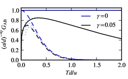
Figure 2: (Color online) Temperature dependence of the amplitude of the dimensionless conductance corresponding to interference oscillation amplitudes, $G=(2\pi n_{F}^{2})^{-1}\mathop{\mathrm{Re}}\,\mathrm{d}Z_{1/2}\,/\mathrm{d}V\,\rvert_{V=0}$. The spin-flip $G_{\rm AB,sf}$ (solid), non-spin-flip $G_{\rm AB}$ (dashed), and the high-temperature scaling from Eq. (5) (dotted) are shown.

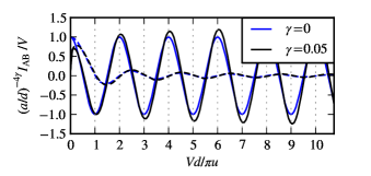
Figure 3: (Color online) Bias dependence of the amplitude of the interference component of the current, for $T=0$. The spin-flip (solid), non-spin-flip (dashed) contributions are shown. Apart from the low-bias power law, the noninteracting ($\gamma=0$, $g=1$) and interacting ($\gamma=0.05$, $g\approx 0.64$) cases differ mainly in the oscillation period $\pi u/d=\pi v_{F}/gd$.

Relation between charge and spin currents. To understand the dephasing in the spin current, it is useful to note first that in a HLL the spin current is closely associated with the charge current. The changes in charge ($c$) and spin ($s$) currents due to tunneling are $\delta I_{c}\propto\delta\rho_{+}-\delta\rho_{-}\,,$ and $\delta I_{s}\propto\delta\rho_{+}+\delta\rho_{-}$ in terms of changes in the densities $\rho$. Note that this spin current is defined with respect to Kramers partners. When evaluated in the noninteracting right (left) lead, in which the $+$ and $-$ modes are independent and $\delta\rho_{-}=0$ ($\delta\rho_{+}=0$) because of ballistic transport, we find $\delta I_{c}^{1R}=\delta I_{s}^{1R}$ and $\delta I_{c}^{1L}=-\delta I_{s}^{1L}$ on the upper edge 1 (positive direction of current is from left to right in Fig. 1). On the lower edge 2, the sign of the spin current is flipped. In a four-terminal setup, this relation becomes more transparent if one considers an XYZ decomposition teo2009-cbo of the currents, extended to account for possible non-conservation of spin: $I^{X}=\frac{1}{2}[I^{1L}+I^{2L}+I^{1R}+I^{2R}]$ indicates the total current flowing from the left (L) to the right (R), $I^{Y}=\frac{1}{2}[I^{1L}-I^{1R}-I^{2L}+I^{2R}]$ the total current from top to bottom, $I^{Z}=\frac{1}{2}[I^{1L}+I^{1R}-I^{2L}-I^{2R}]$ the current flowing between the diagonals, and $I^{S}=-I^{1L}-I^{2L}+I^{1R}+I^{2R}$ the non-conserving “source” current flowing out of the system. In this representation we find:

$$\begin{pmatrix}\delta I_{s}^{X}\\ \delta I_{s}^{Y}\\ \delta I_{s}^{Z}\\ \delta I_{s}^{S}\end{pmatrix}=\begin{pmatrix}0&-1&0\\ -1&0&0\\ 0&0&0\\ 0&0&2\end{pmatrix}\begin{pmatrix}\delta I_{c}^{X}\\ \delta I_{c}^{Y}\\ \delta I_{c}^{Z}\end{pmatrix}\,,$$ (6)

since the dc charge current is conserved ($I_{c}^{S}=0$). The result applies to any helical four-terminal setup. Note that the spin current flows perpendicular to the charge current, which is a signature of the spin-Hall effect giving rise to the helical state. As a result, the spin current can be accessed by a measurement of the transverse charge current.

Spin tunneling current. From Eq. (6) it immediately follows that also spin currents suffer from $e$-$e$ interaction induced dephasing. For instance, consider the spin tunneling current (Y) that can be generated by applying a bias $V_{s}$ between left and right (X), $\mu_{1+}=\mu_{2+}=V_{s}/2$, $\mu_{1-}=\mu_{2-}=-V_{s}/2$. In this configuration, there is no (Y)-charge current strom2009-tbe , similarly as in the (Y)-bias configuration where there was no spin (Y)-current. Here, the spin current is given by the difference between particle currents tunneling into the $+$ and $-$ channels, and it can be directly evaluated using Eq. (4): $\langle{\hat{I}_{T,s}}\rangle=\langle{-\hat{I}_{+}+\hat{I}_{-}}\rangle=I_{s}^{\rm direct}+I_{s}^{\rm AB}$. To leading order in $H_{T}$, the spin (Y)-tunneling current has the same form as the charge (Y)-tunneling current in the Y-biasing configuration (see Eq. (5a)), except that in this order in $H_{T}$, spin-flipping tunneling cannot contribute .

Depending on the interaction parameter $g$ and the amount of spin-flips in tunneling, the interference contribution in spin current can at high temperatures be dominated by two-particle tunneling processes (see Fig. 4), as described by the effective Hamiltonian (cf. teo2009-cbo ),

$$H_{T}^{(2)} =v_{\rho}\psi_{1+}\psi_{2-}^{\dagger}\psi_{2+}\psi_{1-}^{\dagger}$$ (7)

$$+v_{\rho,sf}\sum_{i\neq{}j}\psi_{i,+}\psi_{i,-}^{\dagger}[\psi_{j,+}^{\dagger}\psi_{j,+}-\psi_{j,-}^{\dagger}\psi_{j,-}]+\mathrm{h.c.}\,.$$

The spin-density fluctuation assisted backscattering process $v_{\rho,sf}$, which is present only when spin flips are allowed, has a slower dephasing than single particle processes in the whole range $1/2<g<1$: $I_{s}^{\rho,sf,\rm AB}\propto V_{s}\cos(V_{s}d/u)\cos(2k_{F}d+\varphi_{0})\exp(-2gzd)$. The spin-conserving process $v_{\rho}$ on the other hand dominates the single-particle one only for $g<1/\sqrt{3}$: $I_{s}^{\rho,\rm AB}\propto\sin(2V_{s}d/u)\cos(4k_{F}d+\varphi_{0})\exp(-4gzd)$. Although these processes do not transport charge between the two edges nor couple to the flux $\Phi$, the oscillation with the bias $V_{s}$ and $k_{F}$ remains.

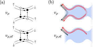
Figure 4: (Color online) Dominant (neutral) compound tunneling contributions to spin interference (Y)-current in (X)-bias configuration. (a) Illustrations of compound processes. The process $v_{\rho}$ conserves spin, whereas process $v_{\rho,{\rm sf}}$ flips one spin. (b) The dynamical phase differences of interfering paths for these compound terms with arrows describing the propagation directions of electrons [filled dots in (a)].

Note that the above implies that in a four-terminal HLL setup, charge and spin tunneling currents have different dephasing exponents, as the interference contribution is dominantly carried by different types of excitations: Neutral electron-hole excitations [Eq. (7)] for $g<1$ have different correlation lengths compared to single-particle excitations. Consider, for instance, the single-particle dephasing exponent $[1+(\frac{g+g^{-1}}{2}-1)]2zd$ from Eq. (5a) compared to the $v_{\rho}$ process, $4gzd=[1-(1-g)]4zd$, where $2zd$ and $4zd$ arise from dynamical phase differences [cf. Fig. 4(b)]. Interestingly, for $v_{\rho}$ the repulsive interaction reduces the dephasing from the noninteracting value.

The above should be contrasted to what occurs in usual SFLLs. There, cotunneling of electrons can create an uncharged spin excitation (spinon), which does not couple to interactions. The lowest-order tunneling process coupling only to the spin sector is the two-electron process

$$H_{T}^{(2s)}=v_{\sigma}L^{2}\sum_{\sigma=\uparrow,\downarrow,\alpha}\psi_{1,\alpha,\sigma}^{\dagger}\psi_{2,\alpha,\sigma}\psi_{2,\alpha,-\sigma}^{\dagger}\psi_{1,\alpha,-\sigma}+\mathrm{h.c.}\,,$$ (8)

where opposite spins tunnel to opposite edges. A calculation along the same lines as above yields the interference component in the spin tunneling current,

$$I_{s,\mathrm{osc}}=4\pi n_{F}^{4}|v_{\sigma}|^{2}V_{s}^{\prime}[(V_{s}^{\prime})^{2}+(2\pi T)^{2}]\cos(V_{s}^{\prime}d/v_{F})\,,$$ (9)

where $V_{s}^{\prime}=\mu_{1\uparrow}-\mu_{1\downarrow}-\mu_{2\uparrow}+\mu_{2\downarrow}$. Exponential dephasing is indeed absent, as expected under SU(2) spin symmetry. Generating such spin currents requires a “spin bias” $V_{s}^{\prime}$, which in our model is essentially equivalent to a difference in spin densities between the two edges. In SFLLs one possibility for inducing this is to contact the SFLL to a system in which a spin imbalance is externally maintained zutic2004-sfa , or to couple it to a HLL liu2010-cdi which may also allow measuring the spin currents via charge currents.

In summary, we showed how electron-electron interaction results in dephasing of interference oscillations in 1D helical liquids, both in charge and spin tunneling currents, with respective exponents that can differ. Moreover, we pointed out how the close coupling of the spin current to the charge current in a helical liquid can result in a qualitatively different behavior from spinful Luttinger liquids. Such effects provide a clear signature of the helicity of the transport, and understanding them may be valuable for applications.

We thank B. Trauzettel and T. Ojanen for useful discussions, and acknowledge financial support from the Emmy-Noether program of the DFG.

Appendix A Current operators

In this work we are interested only in the time-averaged spin or charge currents entering the noninteracting leads. To compute them conveniently, we need to identify the operators corresponding to the tunneling currents, taking into account the plasmon reflections at the edges of the leads.

The identification can be done using a similar approach as in Ref. safi1995-tts . From the Heisenberg equation of motion for the field $\phi$, under a Hamiltonian $H=H_{0}+V[\phi,\vartheta]$, where the effective tunneling term $V$ has support only in a finite region, one finds an exact result for the change in the charge current operator $\delta{\hat{I}}_{c}=\pi^{-1/2}v_{F}\partial_{x}(\phi-\phi\rvert_{V=0})$ in the Heisenberg picture:

$$\delta\hat{I}_{c}(x,t) =v_{F}\int_{-\infty}^{\infty}\mathrm{d}t\,^{\prime}\mathrm{d}x\,^{\prime}\sum_{\alpha=\pm}\alpha\biggl{(}\frac{1+g}{2g}D_{\alpha}(xt,x^{\prime}t^{\prime})$$ (10)

$$\;-\frac{1-g}{2g}D_{-\alpha}(xt,x^{\prime}t^{\prime})\biggr{)}\hat{j}_{\alpha}(x^{\prime}t^{\prime})\,,$$

$$\hat{j}_{\alpha}(x^{\prime}) =\frac{1}{2\sqrt{\pi}}\Bigl{(}\frac{\delta V}{\delta\phi(x^{\prime})}+\alpha\frac{\delta V}{\delta\vartheta(x^{\prime})}\Bigr{)}\,,$$ (11)

where $D_{\pm}$ are solutions to the plasmon wave equation $\partial_{t}^{2}D-\partial_{x}(v_{F}^{2}g(x)^{-2}\partial_{x}D)=0$ with initial conditions corresponding to right (left) moving $\delta$-pulses starting at $x=x^{\prime}$: $D_{\pm}(x,t^{\prime},x^{\prime},t^{\prime})=\delta(x-x^{\prime})$, $\partial_{t}D_{\pm}(x,t^{\prime},x^{\prime},t^{\prime})=\mp{}u\delta^{\prime}(x-x^{\prime})$. Reflections at the lead edges where $g(x)$ changes split the initial pulse to a train of pulses escaping to the leads. Solving the wave equation, one can verify that the fraction of an initially right-going pulse entering the right (left) lead in the long-time limit is $w_{R+}=\lim_{x\to\infty}\int_{0}^{\infty}\mathrm{d}(t-t^{\prime})\,D_{+}(x,t,x^{\prime},t^{\prime})=(1+g)/2$ [$w_{L+}=(1-g)/2$]. Because

$$\frac{1+g}{2g}\frac{1+g}{2}-\frac{1-g}{2g}\frac{1-g}{2}=1\,,$$ (12)

$$\frac{1+g}{2g}\frac{1-g}{2}-\frac{1-g}{2g}\frac{1+g}{2}=0\,,$$ (13)

Eq. (10) leads to the conclusion that (i) all current injected in the $+$ ($-$) channel enters in the right (left) lead, in the time average, and, (ii) $\hat{I}_{\alpha}=\int\mathrm{d}x^{\prime}\,\hat{j}_{\alpha}(x^{\prime})$ is the operator corresponding to the total current injected into channel $\alpha$.

Several other points can also be directly read off (10): since the fluctuation of spin density in a helical liquid is proportional to the same operator $\delta\rho_{+}-\delta\rho_{-}$ as the charge current, it can be seen that a spin injected to a helical liquid fractionalizes into counterpropagating plasmons carrying the fractional spin $(g\pm{}1)/2g$ (cf. das2010-sps ). A similar calculation for the charge density fluctuation implies that an injected electron fractionalizes to plasmons carrying the charge $(1\pm{}g)/2$, as usual pham2000-fei . The equation also guarantees that similarly as charge, a spin injected to the $+$ ($-$) channel will, in the long-time limit, be transmitted in entirety to the right (left) lead. This implies that spin fractionalization cannot be detected by simple time-averaging spin current measurements (such as those proposed e.g. in das2010-sps ), but instead one needs to have access to time scales of $gl/v_{F}$ characteristic of the plasmon transport.

Appendix B Scaling dimensions and dephasing

The limiting behavior of dephasing of interference effects at low or high temperatures can be found from an analysis of the scaling dimensions of the terms in the effective tunneling Hamiltonian.

Given a bosonized operator $M=ve^{in\sqrt{\pi}(\phi+\vartheta)}e^{iq\sqrt{\pi}(\phi-\vartheta)}$ (on a single edge), within our model one finds the correlation function

$$\langle{M(x,t)M(0,0)^{\dagger}}\rangle_{0}\propto{}|v|^{2}F(x,t)^{2\Delta_{+}}(F(x,-t)^{*})^{2\Delta_{-}}\,,$$ (14)

$$\Delta_{+}(n,q)=\frac{[(1-g)n+(1+g)q]^{2}}{8g}=\Delta_{-}(q,n)\,,$$ (15)

where $F(x,t)=iaz/\sinh[z(x-ut-ia)]$, $z=\pi T/u$, and $a$ is the short-distance cutoff length. The scaling dimension of operator $M$ is $\Delta=\Delta_{+}+\Delta_{-}$. Now, if $M$ represents an effective tunneling term in the Hamiltonian, a similar Kubo calculation as done below indicates that at low temperatures its contribution to spin/charge conductance scales as $G\propto|v|^{2}T^{2\Delta-2}$, but at high temperatures $Td/u\gg 1$ interference effects dephase as $G\propto{}e^{-4\pi Td\Delta_{d}}$, where the dephasing exponent $\Delta_{d}=\min[\Delta_{+},\Delta_{-}]$ can differ from $\Delta/2$.

Comparing $\Delta_{d}$ between effective tunneling processes allows us to identify those dominating at high temperatures, and results for the scaling dimension $\Delta$ indicate the magnitude of the tunneling element, and justify the use of perturbation theory.

For $1/2<g<2$ we have $\Delta\geq 1$ for all time-reversal symmetric processes, so that in view of renormalization group flow, the situation is perturbatively stable, and tunneling scales to zero at low energies teo2009-cbo ; hou2009-cja . Concerning dephasing of interference effects, of the tunneling processes transporting charge, we find that at high temperatures the single-particle process dominates (for $g>1/2$),

$$\psi_{1+}\psi_{2+}^{\dagger}\,,\qquad\Delta_{d}=(g+g^{-1})/4-1/2\,.$$ (16)

If spin flips are not allowed, the dominant process is still a single-particle one

$$\psi_{1+}\psi_{2-}^{\dagger}\,,\qquad\Delta_{d}=(g+g^{-1})/4\,,$$ (17)

and the situation stays the same in the whole range $1/2<g<2$.

For spin transport, the situation is considerably different: suppose first that spin is conserved. Then, for $1/\sqrt{3}<g<\sqrt{3}$ single-particle tunneling dominates,

$$\psi_{1+}\psi_{2-}^{\dagger}\,,\qquad\Delta_{d}=(g+g^{-1})/4\,,$$ (18)

but for $1/2<g<1/\sqrt{3}$ a two-particle cotunneling process has the lowest exponent,

$$\psi_{1+}\psi_{2-}^{\dagger}\psi_{2+}\psi_{1-}^{\dagger}\,,\qquad\Delta_{d}=g\,.$$ (19)

In this case, it occurs that $\Delta_{d}=\Delta/2$.

If spin flips are allowed, one finds that the process with the smallest $\Delta_{d}$ in the whole range $1/2<g<1$ is in fact a two-particle one,

$$\psi_{1+}\psi_{2+}^{\dagger}\psi_{2+}\psi_{1-}^{\dagger}\,,\qquad\Delta_{d}=g/2\,.$$ (20)

Note that (i) this process is not important for the charge tunneling current, since it does not transport charge, and (ii) it is higher order in tunneling and has a larger scaling dimension $\Delta=1+g$ than the single particle process. Note that it can also be written in the explicitly time reversal symmetric form $\psi_{1+}\psi_{1-}^{\dagger}[\psi_{2+}^{\dagger}\psi_{2+}-\psi_{2-}^{\dagger}\psi_{2-}]+\mathrm{h.c.}$ resembling spin density fluctuation assisted backscattering.

From the above discussion, we conclude that the leading results for charge tunneling (Y) current are obtained with first-order perturbation theory, but for spin current also second-order contributions, or alternatively, the effective 2-particle tunneling, needs to be analyzed.

Appendix C Kubo correlators

The correlation functions $Z_{1}$, $Z_{2}$ appearing in the Kubo calculation are

$$Z_{1}(x,\omega) =iL^{2}\int_{-\infty}^{\infty}\mathrm{d}t\,e^{i\omega t}\bigl{\langle}[\psi_{1,+}^{\dagger}(x,t)\psi_{2,+}(x,t),$$ (21)

$$\qquad\psi_{2,+}^{\dagger}(0,0)\psi_{1,+}(0,0)]_{-}\bigr{\rangle}_{0}\,,$$

$$Z_{2}(x,\omega) =iL^{2}e^{2ik_{F}x}\int_{-\infty}^{\infty}\mathrm{d}t\,e^{i\omega t}\bigl{\langle}[\psi_{1,+}^{\dagger}(x,t)\psi_{2,-}(x,t),$$ (22)

$$\qquad\psi_{2,-}^{\dagger}(0,0)\psi_{1,+}(0,0)]_{-}\bigr{\rangle}_{0}\,.$$

These correlators can be evaluated via standard bosonization techniques for spinless Luttinger liquids giamarchi2004-qpi

$$Z_{1}(x,\omega) =2in_{F}^{2}v_{F}^{2}a^{-2}\int_{-\infty}^{\infty}\mathrm{d}t\,e^{i\omega t}\mathop{\mathrm{Im}}\biggl{[}\Bigl{(}\frac{iaz}{\sinh\bigl{(}z(x-ut+ia)\bigr{)}}\Bigr{)}^{2\gamma+2}\Bigl{(}\frac{-iaz}{\sinh\bigl{(}z(x+ut-ia)\bigr{)}}\Bigr{)}^{2\gamma}\biggr{]}\,,$$ (23a)

$$Z_{2}(x,\omega) =2in_{F}^{2}v_{F}^{2}a^{-2}\int_{-\infty}^{\infty}\mathrm{d}t\,e^{i\omega t}\mathop{\mathrm{Im}}\biggl{[}\Bigl{(}\frac{iaz}{\sinh\bigl{(}z(x-ut+ia)\bigr{)}}\Bigr{)}^{2\gamma+1}\Bigl{(}\frac{-iaz}{\sinh\bigl{(}z(x+ut-ia)\bigr{)}}\Bigr{)}^{2\gamma+1}\biggr{]}\,.$$ (23b)

Here, $a$ is the short-distance cutoff, $\gamma=\frac{1}{4}(g+g^{-1})-\frac{1}{2}$, $u=v_{F}/g$ is the plasmon velocity, $z=\pi T/u$ the inverse thermal length, and $n_{F}=L/(2\pi v_{F})$ the density of states at the Fermi energy.

Integrals of the above type can be evaluated in closed form by making use of the binomial series

$$\left(\frac{i}{\sinh\xi}\right)^{\alpha}=2^{\alpha}i^{\alpha(\mathop{\mathrm{sgn}}\mathop{\mathrm{Re}}\xi)}\sum_{n=0}^{\infty}\frac{\Gamma(\alpha+n)}{n!\Gamma(\alpha)}e^{-(\alpha+2n)(\mathop{\mathrm{sgn}}\mathop{\mathrm{Re}}\xi)\xi}\,,$$ (24)

and its Fourier transform. In the limit $a\equiv\mathop{\mathrm{Im}}\xi\to 0^{+}$ one finds

$$\int_{-\infty}^{\infty}\mathrm{d}t\,e^{i\omega t}\left(\frac{i}{\sinh(ia-t)}\right)^{\alpha}$$ (25)

$$\simeq\frac{\frac{2^{\alpha}\pi^{2}}{\Gamma(\alpha)}e^{\pi\omega/2}}{\Gamma(1+\frac{i\omega}{2}-\frac{\alpha}{2})\Gamma(1-\frac{i\omega}{2}-\frac{\alpha}{2})[\cosh(\pi\omega)-\cos(\pi\alpha)]}\,,$$

which has simple poles at $\omega=i\alpha+2in$, $n=0,1,2,\ldots$. We now rewrite (23) in the form $f(\omega)-f(-\omega)^{*}$, where $f$ is a convolution that can be transformed via contour integration to a Matsubara sum, which can be evaluated. As a result, we find

$$Z_{1}(x,\omega) =\frac{4^{2\gamma+1}\pi n_{F}^{2}v_{F}^{2}z(az)^{4\gamma}}{u}i\Biggl{(}\frac{e^{-4\gamma xz}}{\Gamma(2+2\gamma)}e^{i\omega x}\Gamma(1+2\gamma-\frac{i\omega}{2uz}){}_{2}\tilde{F}_{1}(2\gamma,1+2\gamma-\frac{i\omega}{2uz},-\frac{i\omega}{2uz},e^{-4xz})$$ (26)

$$\qquad-\frac{e^{-4(\gamma+1)xz}}{\Gamma(2\gamma)}e^{-i\omega x}\Gamma(1+2\gamma+\frac{i\omega}{2uz}){}_{2}\tilde{F}_{1}(2+2\gamma,1+2\gamma+\frac{i\omega}{2uz},2+\frac{i\omega}{2uz},e^{-4xz})\Biggr{)}\,,$$

$$\mathop{\mathrm{Re}}Z_{2}(x,\omega) =\frac{4^{2\gamma+1}2\pi n_{F}^{2}v_{F}^{2}z(az)^{4\gamma}}{u}\frac{e^{-4(\gamma+1/2)xz}}{\Gamma(1+2\gamma)}\mathop{\mathrm{Im}}\bigl{[}e^{i\omega x}\Gamma(1+2\gamma-\frac{i\omega}{2uz}){}_{2}\tilde{F}_{1}(1+2\gamma,1+2\gamma-\frac{i\omega}{2uz},1-\frac{i\omega}{2uz},e^{-4xz})\bigr{]}\,,$$ (27)

where ${}_{2}\tilde{F}_{1}(a,b,c,z)={}_{2}F_{1}(a,b,c,z)/\Gamma(c)$ is the regularized hypergeometric function. For $z\gg{}1/d$ and $V\ll{}T$ we obtain Eqs. (5a) and (5b) of the main text.

Appendix D Compound tunneling between HLLs

The spin transport due to the compound tunneling Hamiltonian

$$H_{T}^{(2)} =v_{\rho}\psi_{1+}\psi_{2-}^{\dagger}\psi_{2+}\psi_{1-}^{\dagger}$$ (28)

$$+v_{\rho,sf}\sum_{i\neq{}j}\psi_{i,+}\psi_{i,-}^{\dagger}[\psi_{j,+}^{\dagger}\psi_{j,+}-\psi_{j,-}^{\dagger}\psi_{j,-}]+\mathrm{h.c.}\,.$$

can be handled similarly as above. For $H_{T}=v_{\rho}\psi_{1+}\psi_{1-}^{\dagger}\psi_{2+}\psi_{2-}^{\dagger}+\mathrm{h.c.}$ we find $I_{+}=-I_{-}=2iv_{\rho}\psi_{1+}\psi_{1-}^{\dagger}\psi_{2+}\psi_{2-}^{\dagger}+\mathrm{h.c.}$ on the basis of Eq. (11). From this we immediately see that in the X-bias configuration the charge (Y) current vanishes, and the spin (Y) current is obtained by a straightforward calculation:

$$\langle{I_{T,s}}\rangle =2\sum_{R=0,d}|v_{\rho}(R)|^{2}\mathop{\mathrm{Re}}{}Z_{3}(0,-2V_{s})$$ (29)

$$\quad+4\mathop{\mathrm{Re}}[v_{\rho}(0)v_{\rho}(d)^{*}e^{4ik_{F}d}]\mathop{\mathrm{Re}}{}Z_{3}(d,-2V_{s})\,,$$

$$Z_{3}(x,\omega) =(2\pi a)^{-2}Z_{2}(x,\omega)\rvert_{\gamma\mapsto{}g-1/2}\,.$$ (30)

Apart from the prefactor, the result is identical to $Z_{2}$ with a different exponent, in agreement with Eq. (14).

Similarly, starting from

$$H_{T}^{(2)}=\sum_{i\neq{}j}v_{\rho,sf}\psi_{i,+}\psi_{i,-}^{\dagger}[\psi_{j,+}^{\dagger}\psi_{j,+}-\psi_{j,-}^{\dagger}\psi_{j,-}]+\mathrm{h.c.}\,,$$ (31)

we get $I_{1+}=-I_{1-}=2iv_{\rho,sf}\psi_{1+}\psi_{1-}^{\dagger}[\psi_{2+}^{\dagger}\psi_{2+}-\psi_{2-}^{\dagger}\psi_{2-}]+\mathrm{h.c.}\equiv{}iM_{1}-iM_{1}^{\dagger}$, and similarly on edge 2. The relevant correlation functions are of the form

$$\langle{M_{1}(r,t)M_{1}^{\dagger}(0,0)}\rangle_{0}\propto|v_{\rho,\rm sf}|^{2}e^{-i(\mu_{1+}-\mu_{1-})t}e^{2ik_{F}r}$$ (32)

$$\;\times F(r,t)^{g}(F(r,-t)^{*})^{g}[F(r,t)^{2}+(F(r,-t)^{*})^{2}]\,,$$

which implies that the high-temperature dephasing exponent is $\Delta_{d}=g/2$, being different from $\Delta/2=g/2+1$. We remark that the contribution in third order in tunneling vanishes identically due to particle conservation.

Note that in the X-bias configuration, we have $\delta I_{c}^{X}=2I_{+}$, $\delta I_{c}^{Y}=0$, and $\delta I_{c}^{Z}=0$ for both of the above processes.

Appendix E Description of SFLL

In a spinful Luttinger liquid giamarchi2004-qpi , the direction of spin and motion is not coupled and the fermion operator has to be defined separately for spin and direction of motion (at each edge):

$$\psi_{\alpha,\uparrow(\downarrow)}(x)\simeq e^{i\alpha[k_{F}x+\sqrt{\pi}\vartheta_{\uparrow(\downarrow)}(x)]+i\sqrt{\pi}\phi_{\uparrow(\downarrow)}(x)}\,.$$ (33)

It is advantageous to change to charge ($\rho$) and spin ($\sigma)$ variables $\phi_{\uparrow(\downarrow)}=(1/\sqrt{2})(\phi_{\rho}\pm\phi_{\sigma})$ and $\vartheta_{\uparrow(\downarrow)}=(1/\sqrt{2})(\vartheta_{\rho}\pm\vartheta_{\sigma})$, explicitly

$$\psi_{\alpha,\sigma}(x)\simeq e^{i\alpha k_{F}x}e^{i\sqrt{\frac{\pi}{2}}(\phi_{\rho}+\alpha\vartheta_{\rho}+s(\phi_{\sigma}+\alpha\vartheta_{\sigma}))}\,,$$ (34)

with $s=\pm$ for $\sigma=\uparrow,\downarrow$. In these new variables, the interacting system generally splits into a sum of spin and charge parts: $H_{\rm SFLL}=H_{\rho}+H_{\sigma}+g_{1}\int_{-\infty}^{\infty}dx\cos(\sqrt{8\pi}\vartheta_{\sigma})$. These Hamiltonians are characterized by interaction parameters $g_{\nu}$ and velocities $v_{\nu}$, $\nu=\rho,\sigma$. At the low-energy fixed point, $g_{1}$ flows to zero for repulsive SU(2) invariant interactions and therefore the Hamiltonian becomes $H=H_{\rm SLL}=H_{\rho}+H_{\sigma}$ with

$$H_{\rho}=\frac{u_{\rho}}{2}\int_{-\infty}^{\infty}dx\left[g_{\rho}\left(\partial_{x}\phi_{\rho}\right)^{2}+\frac{1}{g_{\rho}}\left(\partial_{x}\vartheta_{\rho}\right)^{2}\right],$$ (35)

and

$$H_{\sigma}=\frac{u_{\sigma}}{2}\int_{-\infty}^{\infty}dx\left[g_{\sigma}\left(\partial_{x}\phi_{\sigma}\right)^{2}+\frac{1}{g_{\sigma}}\left(\partial_{x}\vartheta_{\sigma}\right)^{2}\right],$$ (36)

where $g_{\rho}\equiv g$, $u_{\rho}\equiv u$, and $g_{\sigma}=1$ giamarchi2004-qpi . The spin sector therefore becomes effectively non-interacting.

The dephasing for spin currents can therefore be absent in second order in the tunneling which we describe by the effective Hamiltonian

$$H_{T}^{(2s)}=v_{\sigma}L^{2}\sum_{\sigma=\uparrow,\downarrow,\alpha}\psi_{1,\alpha,\sigma}^{\dagger}\psi_{2,\alpha,\sigma}\psi_{2,\alpha,-\sigma}^{\dagger}\psi_{1,\alpha,-\sigma}+\mathrm{h.c.}\,,$$ (37)

e.g. consider the term

$$\psi_{1+\uparrow}\psi_{2+\uparrow}^{\dagger}\psi_{2+\downarrow}\psi_{1+\downarrow}^{\dagger}\sim e^{i\sqrt{\pi/2}(\phi_{1\sigma}+\vartheta_{1\sigma}-\phi_{2\sigma}-\vartheta_{2\sigma})}.$$ (38)

The correlation function of terms like this one will not show fractionalization because $g_{\sigma}=1$ and the charge fields have disappeared from the bosonized expression.

The coupling constant $v_{\sigma}$ in the effective Hamiltonian Eq. (37) is second order in the bare tunneling amplitude and can depend (at low bias voltages) on temperature in a power-law fashion (see section below) but will not depend on the interferometer length $d$ as long as $Td/u\gg{}1$.

Appendix F Renormalization of tunneling operators

For completeness, we now summarize how compound tunneling terms can be derived via the real-space perturbative renormalization group anderson1970-eri , which has proved useful in studies of Luttinger liquids kane1992-ttb ; giamarchi2004-qpi .

We first note that bosonization allows evaluation of correlation functions involving Fermi operators in closed form. In general, for a set of bosonic operators $\Phi_{j}$, a well-known expansion applies:

$$\langle{\mathbb{T}\prod_{i}e^{i\Phi_{i}}}\rangle_{0}=e^{-\frac{1}{2}\sum_{ij}\langle{\mathbb{T}\Phi_{i}\Phi_{j}}\rangle_{0}}\,,$$ (39)

where $\mathbb{T}$ indicates (contour-)time ordering. Given the bosonic correlation functions, $\langle{\Phi_{\pm}(t)\Phi_{\pm}(0)}\rangle_{0}=\frac{1}{2\pi{}g}\ln\{-izL/\sinh[z(t-ia)]\}$ for $\Phi_{\pm}\equiv 2^{-1/2}(\phi\mp\vartheta/g)$, one finds a short-time expansion $\langle{\mathbb{T}A(t)B(t^{\prime})Q}\rangle_{0}\propto|t-t^{\prime}|^{-\alpha}\langle{\mathbb{T}A(t)B(t)Q}\rangle_{0}$ as $t^{\prime}\to{}t$ for groups $A$ and $B$ and $Q$ of Fermi operators. Since the scaling at $t^{\prime}\to{}t$ is independent of $Q$, in view of Eq. (39), this can be understood as an operator product expansion $A(t)B(t^{\prime})=|t-t^{\prime}|^{-\alpha}(AB)(t)$ as $t^{\prime}\to{}t$.

The perturbative renormalization group now proceeds by integrating out all short-time divergences at times $a+\mathrm{d}a\,>|t-t^{\prime}|>a$ appearing in the second order of perturbation expansions. The generated compound terms are absorbed in the first order of the expansion via a change in the Hamiltonian, $H\mapsto{}H+\mathrm{d}H\,$, which after rescaling the cutoff $a\mapsto{}a+\mathrm{d}a\,$ leads to the RG flow equations.

In this approach, we find the flow equations corresponding to the effective Hamiltonian $H_{\rm eff}=H_{0}+H_{T}+H_{T}^{(2)}$,

$$\frac{\mathrm{d}t_{\alpha\beta}\,}{\mathrm{d}\ln a\,} =[1-(g^{-1}+g)/2]t_{\alpha\beta}\,,$$ (40)

$$\frac{\mathrm{d}v_{\rho}\,}{\mathrm{d}\ln a\,} =[2-2g]v_{\rho}-cat_{+-}t_{-+}^{*}\theta(g^{-1}-g)\,,$$ (41)

$$\frac{\mathrm{d}v_{\rho,\rm sf}\,}{\mathrm{d}\ln a\,} =[1-g]v_{\rho,\rm sf}-c^{\prime}at_{++}t_{-+}^{*}\theta(g^{-1}-1)\,,$$ (42)

where the first terms appear, as usual, from the intrinsic cutoff dependence of the operators, $\langle{\prod_{j}e^{i\Phi_{j}}}\rangle_{0}\propto{}a^{\Delta}$, and the latter from the short-time divergences. The factors $c$ and $c^{\prime}$ are numerical constants. Note that the effective Hamiltonian is written in terms of Fermi operators. Moreover, the compound terms above are generated only for repulsive interactions, $g<1$ — for $g\geq 1$ the perturbation expansion does not have the corresponding short-time divergences.

The flow equation can be integrated starting from the bare values $a=a_{0}$, $t_{\alpha\beta}(a_{0})=t_{\alpha\beta}$, $v_{\rho}(a_{0})=v_{\rho,\rm sf}(a_{0})=0$, up to the length scale at which the operator product expansion breaks down. In our case it is the size of the interferometer $d$ or the thermal length $1/z$, whichever is smaller. This yields the scaling of the prefactors with the cutoff (assuming $1/z\ll d$):

$$t_{\alpha\beta} \propto(a_{0}T)^{(g^{-1}+g)/2-1}t_{\alpha\beta}(0)\,,$$ (43)

$$v_{\rho} \propto(a_{0}T)^{\min(2g-1,g^{-1}+g-2)}T^{-1}t_{+-}(0)t_{-+}^{*}(0)\,,$$ (44)

$$v_{\rho,\rm sf} \propto(a_{0}T)^{\min(g,g^{-1}+g-2)}T^{-1}t_{++}(0)t_{-+}^{*}(0)\,.$$ (45)

A similar treatment gives the scaling for the process described by Eq. (37) in a SFLL

$$v_{\sigma} \propto(a_{0}T)^{\min(1,(g^{-1}+g)/2-1)}T^{-1}t_{+\uparrow,+\uparrow}(0)t_{+\downarrow,+\downarrow}^{*}(0)\,,$$ (46)

The result for $v_{\rho}$ coincides with that obtained in Ref. teo2009-cbo for $g<(\sqrt{5}-1)/2$ at which the scaling $2g-1$ of the compound process starts to dominate the scaling $g^{-1}+g-2$ of two single-particle events. The dephasing exponents for the above processes, on the other hand, follow from the arguments in the previous sections, and in general they are independent of the scaling dimensions of the prefactor.